Interferometric imaging of the sulfur-bearing molecules H₂S, SO and CS in comet C/1995 O1 (Hale-Bopp)

Abstract

Context. We present observations of rotational lines of H₂S, SO and CS performed in comet C/1995 O1 (Hale-Bopp) in March 1997 with the Plateau de Bure interferometer of Institut de Radioastronomie Millimétrique (IRAM).

Aims. The observations provide informations on the spatial and velocity distributions of these molecules. They can be used to constrain their photodissociation rate and their origin in the coma, i.e. nucleus or parent source.

Methods. We use a radiative transfer code which allows us to compute synthetic line profiles and interferometric maps, to be compared to the observations.

Results. Both single-dish spectra and interferometric spectral maps show evidence for a day/night asymmetry in the outgassing. From the analysis of the spectral maps, including the astrometry, we show that SO and CS present in addition a jet-like structure that may be the gaseous counterpart of the dust high-latitude jet observed in optical images. A CS rotating jet is also observed. Using the astrometry provided by continuum radio maps obtained in parallel at IRAM, we conclude that there is no need to invoke the existence of nongravitational forces acting on this comet, and provide an updated orbit. The radial extension of H₂S is found to be consistent with direct release of H₂S from the nucleus. SO displays an extended radial distribution. Assuming that SO₂ is the parent of SO, the photodissociation rate of SO is measured to be $1.5\times 10^{-4}\,\mathrm{s}^{-1}$ at 1 AU from the Sun. This is lower than most laboratory-based estimates and may suggest that SO is not solely produced by SO₂ photolysis. From the observations of $J$(2–1) and $J$(5–4) CS lines, we deduce a CS photodissociation rate of $1-5\times 10^{-5}\,\mathrm{s}^{-1}$. The photodissociation rate of CS₂, the likely parent of CS, cannot be constrained due to insufficient angular resolution, but our data are consistent with published values.

Conclusions. These observations illustrate the cometary science that will be performed with the future ALMA interferometer.

1 Introduction

Spectroscopic investigations of comets in the microwave wavelengths domain began in the 80’s when sensitive instrumentation was made available. This wavelength range proved to be a powerful tool to identify and measure the relative abundances of parent molecules released from comet nuclei from the observations of their rotational lines (see, e.g., the review of Bockelée-Morvan et al. 2004). However, little information was obtained on their spatial distribution in the inner coma because of the poor angular resolution (typically $10\arcsec$ at most) offered by single dish (diffraction-limited) measurements. The study of the spatial distribution of parent molcules is of strong interest as inferences concerning the outgassing processes at the nucleus surface can be made. In addition, the study of the brightness radial distribution of molecular species can provide information on their origin, i.e. indicate whether they are indeed released by the nucleus or produced by some source in the coma. Such investigation has been performed for decades on radicals and atoms observed at visible or UV wavelengths (see the review of Feldman et al. 2004) and provided measurements of their photodissociative lifetime and the lifetime of their parents. Spatial 1-D mapping at high angular resolution has also been undertaken for a few molecules (CO, HCN, H₂O) observed at infrared wavelengths in comets C/1996 B2 (Hyakutake) and/or C/1995 O1 (Hale-Bopp) (e.g., DiSanti et al. 2001; Magee-Sauer et al. 1999).

Mapping of rotational emission lines at high angular resolution was only attempted in a few comets, mostly in comets Hyakutake and Hale-Bopp. Because of their exceptional brightness, interferometric imaging of molecular lines could be successfully performed (e.g., Wright et al. 1998; Blake et al. 1999; Woodney et al. 2002). We present here observations of three sulfur bearing species undertaken in comet Hale-Bopp in March 1997 using the IRAM Plateau de Bure interferometer at angular resolution of 1.6 to 3.5$\arcsec$. H₂S and SO have so far only been detected in comets in the millimetre or submillimetre domains (Bockelée-Morvan et al., 2004). Our observations provide the first study of their spatial distribution. CS has been detected at high angular resolution in the UV in several comets (Feldman et al. 2004). Its spatial distribution was studied in the microwave domain in comet Hale-Bopp using the Berkeley Illinois Maryland Association (BIMA) array (Snyder et al. 2001). Our observations of two CS rotational lines usefully complement these studies.

Section 2 presents the data set. Interferometric images, spectral maps and autocorrelation (i.e., single-dish) spectra of H₂S, SO and CS lines are analysed and compared to investigate jet-like structures and temporal variability linked to nucleus rotation. In Sect. 3, we show that a well-determined gravitational solution for comet Hale-Bopp orbit can be deduced from the astrometry provided by the Plateau de Bure continuum observations. Section 5 focuses on the study of the radial distribution of the molecules, the model being described in Sect. 4. A summary follows in Sect. 6.

2 Observations

2.1 Description

Table 1: Log of the observations and main characteristics.

Line	Date	UT	$r_{h}$	$\Delta$	Mode	$S/{T_{A}}^{\leavevmode\nobreak\ *\mathrm{a}}$	Beam	$\textrm{Line area}^{\mathrm{b}}$	$\Delta\textrm{v}^{\mathrm{c}}$
$\nu$ (GHz)	(1997)		(AU)	(AU)		(Jy/K)	($\arcsec$)	$\textrm{Jy km s}^{-1}$	$\textrm{km s}^{-1}$
CS $J$(2–1)	March 12	8h47–15h30	0.98	1.36	cross	23.5	4.39 $\times$ 2.82	1.47 $\pm$ 0.09	–0.19 $\pm$ 0.020
97.9809533		8h41–14h03			auto	21.1	49.0	15.2 $\pm$ 0.2	–0.06 $\pm$ 0.020
CS $J$(5–4)	March 12	6h31–15h30	0.98	1.36	cross	63.1	1.92 $\times$ 1.28	5.4 $\pm$ 0.8	–0.10 $\pm$ 0.020
244.9355565		6h24-14h03			auto	30.4	19.7	213.2 $\pm$ 0.6	–0.079 $\pm$ 0.003
H2S $2_{20}$–$2_{11}$	March 13	4h25–15h27	0.97	1.35	cross	37.6	1.99 $\times$ 1.53	3.51 $\pm$ 0.15	–0.05 $\pm$ 0.010
216.7104350		4h19-14h37			auto	27.0	22.15	18.9 $\pm$ 0.3	–0.06 $\pm$ 0.020
SO $N_{J}$(56–45)	March 13	4h25–15h27	0.97	1.35	cross	37.6	1.93 $\times$ 1.5	0.44 $\pm$ 0.04	–0.05 $\pm$ 0.090
219.9494420		4h19–14h37			auto	27.0	21.9	16.9 $\pm$ 0.3	–0.13 $\pm$ 0.020

• Conversion factor averaged over the six antennas. Forward and beam efficiencies are ($F_{eff}$, $B_{eff}$) = (0.93, 0.83), (0.89, 0.62), (0.89, 0.55) at 98, 220 and 245 GHz, respectively.

• Intensity integrated over velocity measured in ON–OFF  spectra (autocorrelation mode), and in the central pixel of the interferometric maps (cross-correlation mode). The given uncertainties do not include uncertainties in the absolute calibration ($\sim$ 15% in both modes).

• Line velocity shift defined as $\Delta v=\frac{\sum_{i}T_{i}v_{i}}{\sum_{i}T_{i}}$, where $T_{i}$ and $v_{i}$ are the intensity and velocity of channel $i$, respectively

Comet C/1995 O1 (Hale-Bopp) was observed in 1997 at the IRAM Plateau de Bure Interferometer situated in the french Alps (Guilloteau et al., 1992). The observing campaign lasted 2 weeks between March 6 and March 22, at the time of the closest approach of the comet to the Earth (perigee was on March 22). The programme included interferometric mapping and single dish measurements in spectroscopic mode for several molecular species (CO, HCN, HNC, CS, H₂S, SO₂, SO, CH₃OH, H₂CO; Wink et al. 1999; Bockelée-Morvan et al. 2000; Henry et al. 2002; Henry 2003; Bockelée-Morvan et al. 2005), as well as observations of the dust and nucleus continuum emission (Altenhoff et al. 1999).

At the IRAM Plateau de Bure interferometer, observations with 1.3 and 3 mm receivers were conducted at the same time. The CS $J$(2–1) and $J$(5–4) lines (at 98.0 and 244.9 GHz, respectively) were observed in parallel on March 12. On March 13, the $2_{20}$–$2_{11}$ line of H₂S (at 216.7 GHz) and $N_{J}$(5₆–4₅) line of SO (at 219.9 GHz) were observed simultaneously in the same backend, taking benefit of double-sideband receivers. A log of the observations is presented in Table 1. At this time, the instrument counted five 15-m antennas set in C1 compact configuration so that baseline lengths projected onto the plane of the sky were between 22 m and 147 m. The comet was at a geocentric distance $\Delta=1.35-1.36$ AU and heliocentric distance $r_{h}=0.97-0.98$ AU.

The comet was tracked using orbital elements computed by D.K. Yeomans (JPL ephemeris solution 55) and the ephemeris program of the Institut de mécanique céleste et de calcul des éphémérides (IMCCE, Observatoire de Paris) that takes into account planetary perturbations. First interferometric maps obtained on March 9 showed that the intensities (of both continuum and line emissions) peaked 5–6$\arcsec$ northward with respect to the expected position. The ephemeris was corrected by $+6\arcsec$ in declination (Dec) for the observations performed on March 12 and 13. It turned out that the position of the brightness peaks (continuum and lines) was offset by less than $\sim$2$\arcsec$ with respect to the pointed position. Single dish measurements are not affected by this pointing offset given the size of the primary beam at the observed frequencies (Half Power Beam Width, HPBW, of 22 to 50$\arcsec$, Table 1).

The observing cycle was typically: pointing, focussing, 4 min of cross-correlation on the calibrators, 2 min of autocorrelation (ON–OFF measurements, 1 min on source) and 51 scans (1 min each) of cross-correlation on the comet. At the end of some cycles, additional autocorrelation spectra were obtained. Hereafter, autocorrelation observations will be refered to as “ON–OFF” observations. The OFF position in ON–OFF (position switching) observations was at 5$\arcmin$ from the ON position.

In 1997, the correlator consisted of 6 independent units, adjustable in resolution and bandwidth. On March 12, two units were used for observing CS, the other ones were used for CH₃OH lines near 241 GHz. On March 13, four units were used for measuring the continuum emission (Altenhoff et al. 1999), and one unit covered the $J$(1–0) HNC line observed with the 3 mm receivers (Bockelée-Morvan et al. 2005). Another one covered both the $2_{20}$–$2_{11}$ H₂S and $N_{J}$(5₆–4₅) SO lines present in lower and upper receiver sidebands. The units used for CS, H₂S and SO lines were divided into 256 channels with 78 kHz separation, providing an effective velocity resolution of $\sim 0.31\textrm{\leavevmode\nobreak\ \leavevmode\nobreak\ km\leavevmode\nobreak\ s}^{-1}$ for CS $J$(2–1), $\sim 0.12\textrm{\leavevmode\nobreak\ \leavevmode\nobreak\ km\leavevmode\nobreak\ s}^{-1}$ for CS $J$(5–4) and $\sim 0.13\textrm{\leavevmode\nobreak\ \leavevmode\nobreak\ km\leavevmode\nobreak\ s}^{-1}$ for H₂S and SO lines (the resolution is 1.3 times the channel spacing).

The frequency calibration was checked by observing the reference source W3OH. Interferometric observations were calibrated using the standard IRAM software CLIC. The amplitude and phase calibrator was BL Lac (2200+420) which flux density was determined observing MWC349. In ON–OFF mode, the intensity scale is the antenna temperature ${T_{A}}^{*}$. The conversion factor from ${T_{A}}^{*}$ to flux density and the HPBW of the primary beam at the frequencies of CS, H₂S and SO lines are given in Table 1. The uncertainty in flux calibration is about 15%, both in interferometric and ON–OFF mode.

2.2 ON–OFF spectra

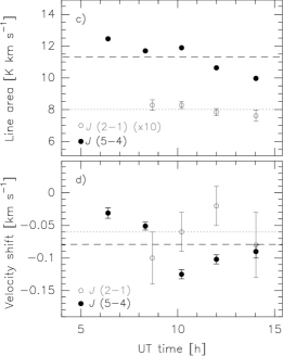
Figure 1: a–b: ON–OFF spectra of CS $J$(5–4) (244.9 GHz) (a) and CS $J$(2–1) (98.0 GHz) (b) lines recorded on March 12, 1997. The spectra, in brightness temperature scale, are shifted vertically according to observation UT time (given in the top right corners). Horizontal lines correspond to zero intensity. The integration time is 2 min (CS $J$(5–4) at 6.40 h and 14.04 h and CS $J$(2–1) at 8.69 h and 14.04 h) or 4 min. The velocity scale is with respect to the comet rest velocity. c: Line area as a fonction of UT time. Black and grey symbols are for $J$(5–4) and $J$(2–1) lines, respectively. The black dashed (respectively grey dotted) line shows mean value for $J$(5–4) (respectively $J$(2–1)) line. d: Line velocity shift as a fonction of UT time. Black and grey symbols are for $J$(5–4) and $J$(2–1) lines, respectively. The black dashed (respectively grey dotted) line shows mean $\Delta v$ value for $J$(5–4) (respectively $J$(2–1)) line.

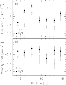
Figure 2: a–b: ON–OFF spectra of H₂S $2_{20}-2_{11}$ (216.7 GHz) (a) and SO $N_{J}$(5${}_{6}-4_{5}$) (219.9 GHz) (b) lines recorded on March 13, 1997. The spectra, in brightness temperature scale, are shifted vertically according to observation UT time (given in the top right corners). Horizontal lines correspond to zero intensity. The integration time is 4 min for all spectra, but those at 4.32 h and 14.62 h UT for which it is 2 min. The velocity scale is with respect to the comet rest velocity. c: Line area as a fonction of UT time. Black and grey symbols are for H₂S and SO, respectively. The black dashed (respectively grey dotted) line shows mean value for H₂S (respectively SO) line. d: Line velocity shift as a fonction of UT time. Black and grey symbols are for H₂S and SO, respectively. The black dashed (respectively grey dotted) line shows mean $\Delta v$ value for H₂S (respectively SO) line.

The ON–OFF spectra obtained independently by the five antennas were co-added. All lines were detected with a signal-to-noise ratio $>$ 10 in single scans, so that the evolution of the line characteristics along the observation period could be studied to investigate possible changes linked to nucleus rotation. Since the rotation period of the nucleus of comet Hale-Bopp is about 11.35 h (e.g., Jorda et al. 1999), the nine H₂S and SO spectra obtained between 4h19 and 14h37 UT (Table 1) spread over almost a full rotation period. Similarly, the observations of CS $J$(5–4) cover 80% of the nucleus period. Technical problems prevented us from obtaining as much time coverage for CS $J$(2–1). Spectra as a function of time are shown in Fig.  1–2.

As shown in Figs. 1–2, no significant temporal changes that could be related to nucleus rotation are observed for the line areas. We also plot in Figs. 1–2 the temporal evolution of the line centroids in nucleus velocity frame, hereafter referred to as line velocity shifts or velocity offsets (see footnote (c) of Table 1). For all molecules, velocity offsets are always negative, taking into account error bars. Given the phase angle on March 12–13 ($\sim 45^{\circ}$), this is consistent with a Sun/anti-Sun asymmetry in the distribution of the molecules, with more molecules towards the Sun. The velocity offsets of the H₂S ($2_{20}$–$2_{11}$), SO $N_{J}(5_{6}$–$4_{5})$ and CS $J$(2–1) lines present some fluctuations but no clear evidence for a 11.35 h periodic modulation (Figs. 1– 2). In contrast, the velocity offset of the CS $J$(5–4) line, measured with much better accuracy (less than 0.01 km s^-1 rms), presents a clear trend of variation with rotation phase, with a minimum on March 12 10h15 UT at $-$0.125 km s^-1, and maximum at $-$0.03 km s^-1 observed 4 h earlier.

These measurements have to be compared to the strong modulation ($\sim$ 0.3 km s^-1 total amplitude) observed on March 11 for the CO $J$(2–1) and $J$(1–0) velocity offsets (the lowest velocity offset of the CO $J$(2–1) line was near 8h30 UT). This modulation has been interpreted as caused by a rotating CO jet emanating from a source near the nucleus equator that was active day and night (Henry et al. 2002; Henry 2003; Bockelée-Morvan et al. in preparation; Boissier et al. 2006), as in mid-March the nucleus rotation axis was near the plane of the sky. The velocity offset of the CO lines took negative to positive values because the velocity vector of the CO-jet with respect to Earth rotated during the course of the observations. Comparing CS and CO lines evolution, one can conclude that their evolution are not in phase, and thus that the CO and CS sources might be different.

The average spectra obtained on March 12 and 13 are shown in Fig. 3. Their characteristics are summarized in Table 1. Comparing the shapes of the lines and their Doppler shift, we can notice that the SO line is more asymmetric than the H₂S line. This will be further discussed in Sect. 2.3.

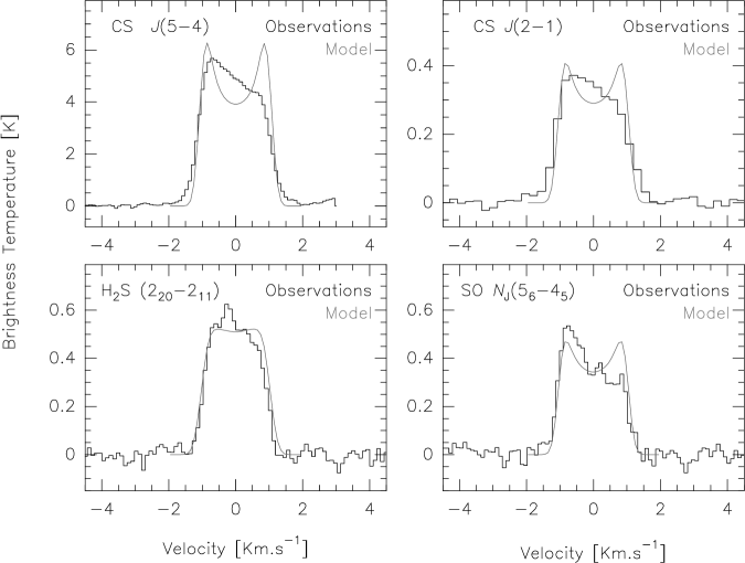
Figure 3: CS $J$(5–4) (244.9 GHz, the integration time (ON+OFF) is 16 min), $J$(2–1) (98 GHz, 12 min), H₂S ($2_{20}$–$2_{11}$) (216.7 GHz, 24 min) and SO $N_{J}$(5₆–$4_{5}$) (219.9 GHz, 24 min) ON–OFF spectra obtained on March 12 and 13, averaging all scans. A typical synthetic profile resulting from the model described in Sect. 4 is overplotted in grey line.

2.3 Interferometric observations

2.3.1 Principle of interferometric imaging

An interferometer measures the 2D Fourier Transform (FT) of the brigthness distribution on the sky. At a time $t$ a pair of antennas provides a point of the FT (a complex number called visibility) at the coordinates ($u,v$) in the Fourier Plane (also called uv–plane), corresponding to the projection on the sky of the baseline (separation between antennas). The baseline projection evolves due to Earth rotation so that a single pair of antennas probes several points of the FT during the observations. At the end of the observing run, the visibilities are stored in a $uv$-table. The final observed sample in the Fourier plane is called uv–coverage.

Interferometric maps are obtained by computing the inverse Fourier Transform of the measured signal. However, because in practice it is impossible to probe the whole Fourier plane, interpolation is required. The asymmetry in the uv–coverage results in an elliptic clean beam. The clean beam (hereafter referred to as interferometric beam) is the central part of the FT of the $uv$–coverage. Direct analysis of the visibilities allows us to avoid the uncertainties due to the interpolation.

2.3.2 CS, H₂S and SO interferometric maps

Figure 4: Interferometric maps of CS $J$(5–4) (244.9 GHz, 5.9 h integration time), $J$(2–1) (98 GHz, 4.7 h), H₂S (216.7 GHz, 6.6 h) and SO (219.9 GHz, 6.6 h) lines on March 12 for CS and 13 for H₂S and SO. Spectral channels covering a velocity interval of 3.67, 4.32, 2.8 and 3.1 $\textrm{\leavevmode\nobreak\ km\leavevmode\nobreak\ s}^{-1}$ centred on comet rest velocity have been considered for CS $J$(5–4), $J$(2–1), H₂S and SO, respectively. The interferometric beam is shown in the left bottom corner (see values in Table 1). The Sun direction is indicated by the arrow. Contours correspond to 10% (respectively 20%) of the peak intensity measured on the centre of the maps for H₂S and CS $J$(2–1) (respectively SO and CS $J$(5–4)).

Table 2: CS, H₂S and SO maximum line brightness positions.

Line	Date	UTa	RAb	Decb	(O-cont)c	(O–C)d
					($\delta$RA,$\delta$Dec)	($\delta$RA,$\delta$Dec)
		h:min:s	h:min:s	∘:$\arcmin$:$\arcsec$	($\arcsec$,$\arcsec$)	($\arcsec$,$\arcsec$)
CS $J$(2–1)	March 12	15:00:00	22:41:28.643	41:36:31.11	e	(+0.42,+2.13)
CS $J$(5–4)	March 12	07:00:00	22:38:43.424	41:24:11.52	e	(+0.37,+2.48)
H2S	March 13	08:00:00	22:47:25.371	42:02:02.88	(+0.06,$+$0.05)	(+0.92,+2.87)
SO	March 13	05:00:00	22:46:21.868	41:57:35.54	($-$0.03,$-$1.34)	(+0.83,+1.48)

• UT time at which coordinates are given.

• Apparent geocentric coordinates of the brightness peak measured on interferometric maps (“O”). Gaussian fits in the $uv$–plane provide similar absolute positions.

• Offset in RA and Dec between molecules brightness peak position (“O”) and 1.3-mm dust continuum peak position (“cont”, Altenhoff et al. 1999). Continuum observations were not performed on March 12.

• Offset in RA and Dec between molecules brightness peak position (“O”) and the comet expected position (“C”) based on astrometric measurements from 27 April 1993 to 4 August 2005 (JPL ephemeris solution 220).

• Continuum observations were not performed on March 12 (Altenhoff et al. 1999).

Figure 5: Position of maximum brightness peaks in molecular maps (plain circles) and 1.3-mm continuum maps (crosses, Altenhoff et al. 1999) with respect to the ephemeris (C) from JPL solution 220. Surrounding ellipses correspond to interferometric beam divided by the signal-to-noise ratio on peak intensity, and indicate the accuracy of the astrometric measurements. The bottom-right panel shows the average continuum offset (cross) and the Sun and rotation axis (N is the nucleus North pole) directions projected onto the plane of the sky.

The interferometric maps, obtained by co-adding the velocity channels where line emission is present, are shown in Fig. 4. The original images have been shifted so that the maximum brightness peaks at the centre of the maps. The main characteristics of these maps (intensity at maximum brightness, absolute and relative coordinates of the peak brightness (O) with respect to current ephemeris (C) and with respect to the position of maximum continuum emission (Cont) measured simultaneously) are summarized in Tables 1 and 2 and Fig. 5. Spectral maps are shown in Figs. 6–8. The following remarks can be done :

• The SO spatial distribution is more extended than that of H₂S. The line flux in the interferometric beam is indeed eight times lower for SO (Table 1), while SO and H₂S lines have comparable intensities in the primary beam, as measured in autocorrelation mode (Fig. 3 and Table 1). Radial distributions will be studied in detail in Sect. 5.

• The points of maximum line brightness do not coincide with the nucleus position provided by the ephemeris (C), found to be 1.5 to 3$\arcsec$ southward (Fig. 5). Similar (O–C) offsets (by typically 1$\arcsec$ in RA and 3$\arcsec$ in Dec) are observed for other lines (CO, HCN, HNC, H₂CO, CH₃OH) mapped at Plateau de Bure (Altenhoff et al. 1999, Bockelée-Morvan et al. in preparation). Continuum maps obtained simultaneously at Plateau de Bure also show a significant trend to peak northward of the ephemeris position, with (Cont–C) offsets in Dec $\sim$+3$\arcsec$ (Altenhoff et al. 1999).

• The positions of H₂S and CO maximum emission match the continuum position. No continuum data were obtained on March 12 at the date of CH₃OH observations, but almost identical (Cont–C) offsets were measured on March 9, 11 and 13 (Fig. 5). Assuming that this (Cont–C) offset applies on March 12, the methanol emission peak also matches the continuum position. In contrast, the point of maximum brightness of other molecules (namely HCN, H₂CO, CS, SO and HNC) lie at intermediate positions between the continuum and the ephemeris.

• In the spectral maps (Figs. 6–8), the lines exhibit larger blueshifts at northward positions with respect to the centre of brightness in the maps. As already noted, blueshifted lines are expected for preferential outgassing towards the Sun. Taking into account the Earth-Comet-Sun geometry, stronger blueshifts towards northern positions is also consistent with a day/night asymmetry. Indeed, though the Sun is towards South in the maps (PA $\sim 160^{\circ}$), a larger number of molecules released from the nucleus illuminated hemisphere are observed to outflow northward rather than southward because the phase angle is $\sim 45^{\circ}$. This was checked by synthesizing spectral maps using the model detailed in Sect. 4 and a Sun/anti-Sun aymmetry in the distribution of the molecules in the coma.

• There are however significant differences between H₂S and SO and CS spectral maps. The H₂S spectra at northern positions are less asymmetric than those of SO and CS at the same positions. In addition, the CS $J$(5–4) spectra at centre and southern positions exhibit excess emission at Doppler velocities around 0 km s^-1. At these velocities, the emitting molecules are moving in (or near) the plane of the sky.

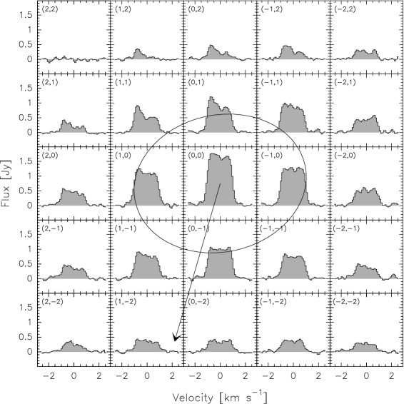
Figure 6: Spectral map of the H₂S ($2_{20}$–$2_{11}$) line. The integration time is 6.6 h. The position of the spectra (RA and Dec offsets in arcsec with respect to the position of maximum brightness) are given in the upper-left corner of the boxes. The ellipse represents the interferometric beam and the arrow indicates the Sun direction projected on the plane of the sky. At northern positions, the blueshifted side of the line is stronger than the redshifted side. Anywhere else the line is overall symmetric.

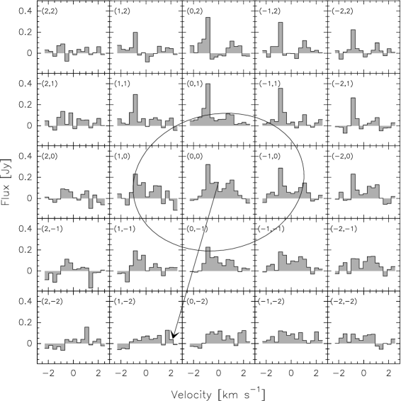
Figure 7: Same figure as Fig 6 for SO $N_{J}$(5₆–4₅) line. The integration time is 6.6 h. In order to improve the signal to noise ratio the spectral resolution has been degraded by a factor 3 and is here about 0.32 km s^-1. The line profile is strongly asymmetric at northern positions, mainly at negative RA offsets.

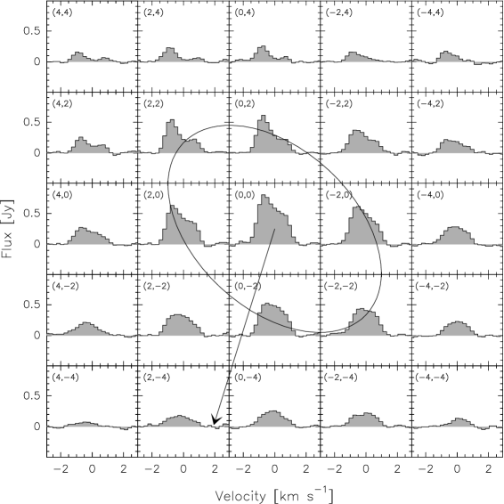
Figure 8: Same figure as Fig. 6 for CS $J$(2–1) (top) and $J$(5–4) (bottom). The integration time is 4.7 and 5.9 h, respectively. At positive Dec offsets (and especially at positive RA), the blueshifted side of the lines is more intense; spectra are globally symmetric at negative Dec offsets. In addition, at zero and negative Dec offsets, $J$(5–4) spectra present a narrow component peaking at $v\sim 0$. Note that the lack of flux in the Dec=$-2\arcsec$ row of CS $J$(5–4) spectral map may be due to the lack of short spacings in the $uv$-plane.

The molecules can be then grouped in two categories: those whose brightness centres coincide with the continuum (H₂S, CO, CH₃OH) and whose spectral maps (averages over about one rotation period) show mainly evidence for a global day/night asymmetry. Molecules of the second group (CS, SO, but also HCN, HNC and H₂CO) have their brightness centres offset towards South with respect to the continuum and may present, in addition to a diurnal asymmetry, a jet-like structure outflowing towards South in the plane of the sky, as observed for CS on its $J$(5–4) spectral maps. Comet Hale-Bopp exhibited in March 1997 a strong dust jet pointing southwest in visible images (Jorda et al. 1999) and interpreted as originating from high latitude regions on the nucleus surface (the rotation axis was at PA $\sim 210^{\circ}$ and aspect angle $\sim 70^{\circ}$ in mid-March 1997, i.e. almost in the plane of the sky, Jorda et al. 1999). We suggest that molecules of the second group present a gaseous counterpart of this dust jet.

On the basis of synthesized maps obtained by describing the coma with a combination of conical structures of various opening angles and, for the continuum, a point-source mimicking nucleus thermal emission, we conclude that: 1) the strong offset (Cont–C) $\sim$ 3$\arcsec$ in Dec cannot be explained by asymmetries in the dust coma, assuming a 50% nucleus contribution to the thermal flux as derived by Altenhoff et al. (1999); the centre of brightness of the continuum maps should be very close (within 0.3$\arcsec$) to the actual position of the nucleus; 2) Sun/anti-Sun asymmetries in the outgassing that are compatible with observed blueshifts cannot displace the centre of molecular line brightnesses by more than a fraction of arcsec, thereby explaining why molecules of the first group have their centre of brightness almost coinciding with the continuum peak (i.e. near nucleus position); 3) the (O–Cont) offsets in Dec observed for the molecules of the second group can be explained by enhanced production in a high-latitude jet-like structure; for CS, a 0.8$\arcsec$ offset is obtained with a model including a wide ($\sim 50^{\circ}$) conical molecular jet oriented in the plane of the sky and comprising about 25% of the total production of CS (Fig. 9); for SO, the 1.4$\arcsec$ offset is obtained with a wider jet ($\sim 80^{\circ}$) containing about 40% of the total production. Such a static wide jet could correspond to the temporal average of a narrower rotating jet; the simulations show that a model combining a diurnal asymmetry and a high-latitude jet reproduces qualitatively the line shapes of CS and SO ON–OFF spectra and spectral maps as well as the (O-Cont) offsets (Fig. 9). 4) the position of the centre of brightness in time-integrated maps is not significantly affected by low-latitude rotating gaseous jets, such as the one observed for CO (Sect. 2.2).

Fitting in detail the H₂S, CS and SO interferometric maps is challenging, given the complexity of Hale-Bopp coma and lack of temporal coverage. This study is beyond the scope of the present paper. In Sect. 5, we will focuss on the radial distribution of these molecules.

Figure 9: Synthetic spectral maps (left panel), ON–OFF spectra (right upper panel) and positions of the brightness maximum with respect to the nucleus (right lower panel) for CS $J$(5–4) (top) and $J$(2–1) (bottom) lines as obtained with a model including a jet like structure southward and a day/night asymmetry in the coma. The jet is 50^∘ wide, and contains about 25 % the total amount of CS. The CS production rate is 5 times stronger in the day side of the nucleus. The arrow indicates the projection of the Sun direction in the plane of the sky. The phase angle is 45^∘.

3 Astrometry: orbital implications

It is at this point useful to discuss the Plateau de Bure observations in the context of the orbit determination of the comet. Whether it is or is not necessary to allow for effects of other than gravitational forces on the Hale-Bopp orbit has long been a rather contentious issue (Marsden, 1999). On the one hand, it was difficult to believe that, active though the comet was, the relative mass loss due to outgassing from a nucleus as large as Hale-Bopp was estimated to be (from 45 to perhaps 70 km diameter, Altenhoff et al. 1999, Weaver & Lamy 1999) would be sufficient to produce a detectable effect on the orbit. On the other hand, as the timespan of the astrometric observations increased well beyond the comet’s perihelion passage, the manner in which the orbital solutions satisfied the data was becoming less and less satisfactory, even when special weighting schemes were introduced to stress some observations over others. Eventually, when the observations extended some ten months after perihelion passage, there was no other possibility but to incorporate nongravitational parameters into the solution, including in particular a radial force component outward from the Sun that had a formal mean error of only some three percent. In broad terms, later orbital solutions, whether computed at the Minor Planet Center or at the Jet Propulsion Laboratory (e.g., MPC 54799 and JPL 220 orbit used in Sect 2.3.2, which both include observations made into Aug. 2005), seemingly confirmed this finding.

If there were a significant departure between the centre of mass and the centre of brightness when the comet was most active, it makes sense to attempt entirely gravitational orbital solutions that exclude consideration of the optical astrometry during that time period. Although the last observations were made more than 12 years after a fortuitous prediscovery observation, some 19 percent of the total of 3565 observations in the Minor Planet Center’s files were made during the 50 days immediately preceding the comet’s perihelion passage. The exclusion of these observations permits a moderately satisfactory gravitational fit to the remainder. The (O–C) residuals in Dec for the omitted timespan are systematically negative to an average extent of about 3$\arcsec$. Only 2 percent of the observations were made during the two months after perihelion passage, but this negative trend also shows during this period of included observations, after which there was a six-week gap in the observational record because of the comet’s small elongation from the Sun. There is likewise a negative trend during the last month of included observations prior to perihelion passage.

Table 3: J2000.0 orbital elements of C/1995 O1 (Hale-Bopp). Epoch 1997 Mar. 13.0 TT.

Orbit	T	q	Peri	Node	Incli.	e	1/a
	1997 Apr. (TT)	(AU)	(∘)	(∘)	(∘)		(AU-1)
I	1.13588	0.9141659	130.58732	282.47062	89.43001	0.9951316	+0.0053255
II	1.13606	0.9141660	130.58734	282.47061	89.43002	0.9951315	+0.0053256
III	1.13623	0.9141657	130.58735	282.47061	89.43003	0.9951313	+0.0053258
	($\pm$ 0.00003)a	($\pm$ 0.0000002)a	($\pm$ 0.00001)a	($\pm$ 0.00001)a	($\pm$ 0.00001)a	($\pm$ 0.0000002)a	($\pm$ 0.0000002)a

• Errorbars for orbit III.

Orbit I in Table 3 was therefore computed from 2693 observations covering the time periods 1995 July 24–1997 Jan. 10 and 1997 July 14–2005 Aug. 4. Observations with a residual in RA or Dec or both of 2.0$\arcsec$ or larger were also excluded from this gravitational solution. The mean residual of the included data is 0.86$\arcsec$, and there are no obvious systematic trends. The single prediscovery observation on 1993 Apr. 27 has an (O–C) Dec residual of -2.0$\arcsec$, and the negative trend during the omitted half-year is much as before.

Table 4: Astrometry of C/1995 O1 (Hale-Bopp) from continuum observations at Plateau de Bure interferometer and residuals with respect to orbits in Table  3.

1997 Mar. UT		RA (J2000.0)	Dec (J2000.0)	(O$-$C) Orbit I	(O$-$C) Orbit II	(O$-$C) Orbit III
				($\delta$RA,$\delta$Dec)	($\delta$RA,$\delta$Dec)	($\delta$RA,$\delta$Dec)
day	h:min:s	h:min:s	∘:$\arcmin$:$\arcsec$	($\arcsec$,$\arcsec$)	($\arcsec$,$\arcsec$)	($\arcsec$,$\arcsec$)
09	05:00:00	22:14:44.864	+39:22:44:07	($-$1.4,$-$0.6)	($-$0.9,$-$0.4)	($-$0.5,$-$0.1)
09	08:00:00	22:15:40.688	+39:27:56.90	($-$1.2,$-$0.6)	($-$0.8,$-$0.4)	($-$0.3,$-$0.1)
09	10:00:00	22:16:18.031	+39:31:24.84	($-$1.2,$-$0.6)	($-$0.7,$-$0.4)	($-$0.2,$-$0.1)
09	12:00:00	22:16:55.459	+39:34:52.18	($-$1.4,$-$0.7)	($-$1.0,$-$0.5)	($-$0.5,$-$0.3)
11	06:00:00	22:30:26.714	+40:45:22.83	($-$1.3,$-$0.6)	($-$0.8,$-$0.5)	($-$0.3,$-$0.2)
11	06:00:00	22:30:26.724	+40:45:23.05	($-$1.2,$-$0.4)	($-$0.7,$-$0.2)	($-$0.2,$-$0.0)
13	08:00:00	22:47:34.109	+42:03:01.56	($-$1.3,$-$0.5)	($-$0.7,$-$0.4)	($-$0.2,$-$0.2)
13	15:00:00	22:50:03.197	+42:13:15.05	($-$1.3,$-$0.5)	($-$0.7,$-$0.3)	($-$0.2,$-$0.2)
16	16:00:00	23:17:10.406	+43:48:28.38	($-$1.1,$-$0.4)	($-$0.5,$-$0.4)	($-$0.0,$-$0.2)
16	16:00:00	23:17:10.407	+43:48:28.42	($-$1.1,$-$0.4)	($-$0.5,$-$0.3)	(+0.1,$-$0.2)

• Continuum geocentric positions from Altenhoff et al. (1999) converted from apparent to J2000.0 coordinates.

The ten IRAM geocentric apparent positions of the peak of the continuum from Altenhoff et al. (1999) are given in Table 4. The first set of residuals shown are from Orbit I, the 2693-observation orbit mentionned above. Although these residuals are systematically negative, the important point is that those in declination are only slightly negative, suggesting that the peak of IRAM continuum emission is substantially closer to the comet’s centre of mass than the optical astrometric observations are during this time. The second set of residuals are from an orbit solution (Orbit II in Table 3) that also includes these IRAM observations. The consistency of the IRAM data suggests it may be appropriate to weight them more heavily in the solution, specifically, by a factor of five. At the same time, it is reasonable to accept in the solution only residuals in either coordinate that are no more than 1.5$\arcsec$. The resulting orbital elements (Orbit III) are given in Table 3. These satisfy 2249 observations with mean residual 0.71$\arcsec$. The residuals of the 1993 and 2005 observations are changed from those of the previous solution by no more than 0.1$\arcsec$. The IRAM residuals from Orbit III are now very commendable.

We conclude that there is no need to invoke the existence of nongravitational forces acting on this comet. The “original” and “future” barycentric values of 1/a are +0.003801 and +0.005571 AU^-1, respectively, corresponding to periods of 4267 and 2405 years.

4 Modelling observations

In order to press on with the data analysis, we have developed a model able to simulate both interferometric and ON–OFF observations of a synthetic coma. In a first step, the brightness distribution of molecular lines in the plane of the sky is computed using a radiative transfer model. This brightness distribution is used in the second step to compute synthetic ON–OFF line profiles and to simulate velocity-resolved interferometric observations.

4.1 Radiative transfer model

Computing the brightness distribution of a molecular rotational line in the plane of the sky is a classical radiative transfer problem that can be easily solved out by numerical integration provided we know: 1) the population distribution of the involved rotational levels; 2) the spatial and velocity distribution of the studied species; 3) the velocity dispersion, assumed here to be thermal at local temperature; and 4) the background emission, taken to be the 2.7 K cosmic background. It also requires an appropriate choice of number of cells and of cell size, both spatially and spectrally, in order to get sufficient accuracy. Detailed formulae of the cells contribution in the case of an optically thin coma can be found in Bockelée-Morvan et al. (in preparation). The code used in this paper is more general as it takes into account opacity effects: in addition to the proper emission of each cell (at given Doppler velocity interval) it computes the cell attenuation of the signal emitted from background cells along the line of sight. The output of the programme is a spectral cube which provides the brightness distribution $F_{i}(x,y)$ in the plane of the sky ($x$,$y$) for a number of velocity channels $i$. The computed map is 256$\times$256 pixels wide, with pixels of $0.5\arcsec\times 0.5\arcsec$, and velocity channels of 0.10 km s^-1.

The level populations in the cells were computed according to the excitation model of Biver et al. (1999). The model takes into account collisions with water molecules and electrons which control excitation in the inner coma: we used a total cross-section for de-excitation by neutral collisions of $1-2\times 10^{-14}$ cm², and a $x_{ne}$ scaling parameter equal to 1 for the electron density. Radiative excitation by the Sun radiation is taken into account for CS (Biver et al. 1999). Radiative excitation is not considered for H₂S and SO molecules. As detailed in Crovisier et al. (1991) and Biver et al. (2006), given their short photodissociation lifetime, they do not undergo significant radiative excitation before being dissociated. This is particularly relevant in March 1997 for comet Hale-Bopp, the collisional region of which was large at this time. The excitation model takes also into account radiation trapping, which main effect is to increase the size of the region where molecules are at thermal equilibrium.

Figure 10: Population of the rotational levels of CS related to observed transitions: J = 1, 2, 4 and 5 as computed with the excitation model. The upper panel corresponds to a constant temperature, the lower to a variable temperature.

Figure 11: Population of the H₂S and SO rotational levels related to observed transitions as computed with the excitation model. The upper panel corresponds to a constant temperature, the lower to a variable temperature.

Because the field of view of the Plateau de Bure observations was essentially sampling molecules with rotational level populations at thermal equilibrium, the temperature of the gas is an important parameter of the model. Both radio (single-dish) (Biver et al. 2002) and infrared (e.g., Magee-Sauer et al. 1999; DiSanti et al. 2001) observations of comet Hale-Bopp in March 1997 suggested gas temperatures $\sim$ 120 K at radial distances of $\sim$10000 km from the nucleus. Evidence for a temperature increase with distance to nucleus is reported from long-slit spectroscopy in the infrared (Magee-Sauer et al. 1999; DiSanti et al. 2001). Such an increase is predicted in coma hydrodynamic simulations as a result of photolytic heating (Combi et al. 1999). Therefore, we investigated two temperature laws in our model:

• a constant temperature: $T=120$ K, derived from the heliocentric dependence of $T$ in comet Hale-Bopp published by Biver et al. (2002).

• a variable temperature: $T=20$ K for $r<100$ km, $T=20+50\log\,(\frac{r\mathrm{[km]}}{100})$ for 100 km $<r<$ 10000 km and $T=120$ K for $r>10000$ km, where $r$ is the radial distance from the nucleus.

The variable temperature law provides a temperature of 70 K at 1000 km from the nucleus, consistent with the model of Combi et al. (1999), but somewhat below the rotational temperatures of 80–90 K derived from infrared measurements with 1$\arcsec$ (1000 km) aperture (Magee-Sauer et al. 1999; DiSanti et al. 2001). Therefore, this temperature law allows us to investigate extreme temperature gradients. The population of the upper and lower levels of the CS, H₂S and SO observed transitions are shown in Figs. 10–11 for the two temperature laws. As the distance from the nucleus increases, the rotational population distributions of the molecules evolve from thermal equilibrium to a cold fluorescence equilibrium, because of declining collision rates. This explains the increase in the outer coma of the population of the levels involved in the observed rotational transitions. With this temperature law, the modelled ON–OFF observations (10000–25000 km field of view radius) mostly probe collisionally excited molecules at $T$ = 120 K, while the interferometric beam (1000 km equivalent radius) is sensitive to colder regions at $T\sim$ 70 K. Colder gas in the inner coma results in larger opacity effects, as it will be shown in Sect. 5.

The radiative transfer code can accommodate any 3-D density and velocity distribution as inputs. For the purpose of Sect. 5, namely the analysis of the radial distribution of CS, H₂S and SO, the density distribution was described by the Haser formulas for parent and/or daughter species. Since the H₂S coma does not show up strong spatial and spectral asymmetries, the assumption of isotropic outgassing is satisfactory for analysing the H₂S data. This is less true for SO and CS (Sect 5), so that this must be kept in mind in the discussion of the results. We can note that the Haser formula for daughter molecules is appropriate for describing the density distribution of SO and CS in comet Hale-Bopp within the IRAM instrumental field of view given the large size ($>$ 10⁵ km, Combi et al. 1999) of the collision sphere in March 1997 compared to the scalelengths of their presumed parents (see Sect. 5). Numerical simulations of asymmetric comas discussed in Sect.2.3.2 were performed using a combination of conical structures, each of them characterized by a production rate by unit of solid angle.

For the gas expansion velocity, we assumed a value about 1.03 $\mathrm{km\leavevmode\nobreak\ s}^{-1}$, derived from the heliocentric dependence of the gas expansion velocity measured in comet Hale-Bopp by Biver et al. (2002). Other relevant parameters in the Haser model that will be constrained by the observations are the photodissociation rates of CS, H₂S, SO and SO parent, and the CS, H₂S and SO production rates.

Table 5: Published photodissociation rates at 1 AU from the Sun.

Molecule	$\beta$ [s-1]	Reference
H2S	$2.5\times 10^{-4}\phantom{\,{}^{\star}}$	Crovisier et al. 1991
CS2	$1.0\times 10^{-5}\phantom{\,{}^{\star}}$	Jackson et al. 1982
	$2.0\times 10^{-5}\phantom{\,{}^{\star}}$	Biver et al. 2003
	$1.0\times 10^{-4}\phantom{\,{}^{\star}}$	Snyder et al. 2001
CS2	$1.0\times 10^{-3}\phantom{\,{}^{\star}}$	Feldman et al. 1999
	$1.7\times 10^{-3}\phantom{\,{}^{\star}}$	Jackson et al. 1986
SO2	$1.5\times 10^{-4}\phantom{\,{}^{\star}}$	Kim & A’Hearn 1991
	$4.9\times 10^{-4}\phantom{\,{}^{\star}}$	Summers & Strobel 1996
	$6.2\times 10^{-4}\phantom{\,{}^{\star}}$	Huebner et al. 1992
SO2	$2.1\times 10^{-4}\phantom{\,{}^{\star}}$	Kim & A’Hearn 1991
	$2.1\times 10^{-4}\phantom{\,{}^{\star}}$	Huebner et al. 1992
	$2.3\times 10^{-4}\phantom{\,{}^{\star}}$	Kumar 1982
	$2.9\times 10^{-4}\,{}^{\star}$	Summers & Strobel 1996

^⋆ The solar spectrum model used pertains to solar maximum.

4.2 ON–OFF synthetic spectra

Synthetic ON–OFF line profiles are readily obtained from the spectral cube by convolving the brightness distribution obtained for each velocity channel with the primary beam pattern. The beam pattern $A(x,y)$ was described by a 2D-gaussian which width at half maximum is equal to the HPBW given in Table 1.

4.3 Synthetic interferometric observations

The simulation of interferometric observations is more complex, as it requires the Fourier transform of the brighness distribution taking into account the uv–coverage (see Sect. 2.3).

For each channel $i$, the visibilities are defined by (see e.g., Thompson et al., 1991) :

$$\mathcal{V}_{i}(\@vec{\sigma})=\frac{c}{\nu\delta v}\int_{4\pi}A(\@vec{s})F_{i}(\@vec{s})\exp(-\frac{2i\pi\nu}{c}\@vec{\sigma}\cdot\@vec{s})d\Omega,$$ (1)

where $\@vec{\sigma}$ is the baseline vector for two antennas, with coordinates ($u$,$v$) in the $uv$-plane. $\@vec{s}$ is a vector in the sky plane which coordinates are $(x,y)$ in radian units. $A$ is the power pattern of the antennas, and $d\Omega$ is an element of solid angle on the sky. Unit of the brightness distribution $F_{i}(x,y)$ provided by the radiative transfer model is [W m^-2 sr^-1]. $\mathcal{V}_{i}(\@vec{\sigma})$ is here in units of [W m^-2 Hz^-1] or janskys. Equation 1 can be approximated to :

$$\mathcal{V}_{i}(u,v) = \frac{c}{\nu\delta v}\int_{-\infty}^{+\infty}\int_{-\infty}^{+\infty}A(x,y)F_{i}(x,y)$$ (2)

$$\times\ \exp(-\frac{2i\pi\nu}{c}(ux+vy))\,dxdy.$$

The calculation of the visibilities is carried out using the GILDAS software collection provided by IRAM. The first step consists in converting the brightness spectral map $F_{i}(x,y)$ times the primary beam gaussian pattern $A(x,y)$ into GILDAS format. Then a GILDAS task computes the Fourier transform according to Eq. 2. In order to simulate data comparable to observations, it is necessary to take into account the uv–plane sampled by the observations. In practice, the GILDAS task reads the $uv$-coverage in the observed data file and computes the $\mathcal{V}_{i}(u,v)$ for each ($u$,$v$) point. This step provides a $uv$-table that can be handled exactly like that recorded during the observations. Modelled and observed maps obtained by inverse Fourier Transform can be compared.

It is also possible to compare the visibilities in the Fourier space. Because of symmetry properties of the Fourier Transform, a radially symmetric brightness distribution results in visibilities $\mathcal{V}_{i}(u,v)$ that only depend upon the $uv$-radius $\sigma$ =$\sqrt{u^{2}+v^{2}}$. Observed visibilities that have been radially averaged in the $uv$-plane can be directly compared to modelled $\mathcal{V}_{i}(\sigma)$. In such a way, the mean (angularly averaged) radial brightness distribution of observed species can be investigated. For this study, visibilities integrated over velocity $\sum_{i}\mathcal{V}_{i}(\sigma)\delta v$ [Jy km s^-1] (with $\delta v$ equal to channel width) will be compared (Sect. 5). Note that the line flux measured in ON–OFF mode corresponds to the visibility at $\sigma$ = 0.

5 Analysis of the radial distribution of CS, H₂S and SO

Two different methods are used to analyse the radial distribution of CS, H₂S and SO. Let us define $F_{\rm SD}$ as the line area of the ON–OFF spectra and $F_{\rm Int}$ as the line area at maximum intensity in the interferometric maps, which observed values are given in Table 1. Because of the factor of $\sim$ 10 difference in angular resolution between ON–OFF and interferometric observations, the flux ratio $R=F_{\rm SD}/F_{\rm Int}$ is strongly sensitive to the spatial distribution. We can thus compare observed and modelled flux ratios to constrain model parameters. The more extended the brightness distribution is, the larger the flux ratio $R$. In the second method, we compare observed and modelled visibilities as a function of $uv$-radius, as explained previously, including the ON–OFF data point.

Input free parameters in the model are photodissociation and production rates. The production rate $Q$ is adjusted iteratively by running the model several times in order to match at best the flux ratio and the observed intensities $F_{\rm SD}$ and $F_{\rm Int}$. Indeed, the intensities (particularly $F_{\rm Int}$) are affected by small but significant opacity effects, so that the flux ratio depends on $Q$.

5.1 Hydrogen sulfide H₂S

Table 6: Observed and modelled fluxes (in Jy km s^-1) and flux ratios.

	Observationsa	Modelsb
		$T=120\,\mathrm{K}$		$T$ variable
		$Thin$	$Thick$	$Thin$	$Thick$
H2S $2_{20}$–$2_{11}$
$F_{SD}$	$18.9\pm 2.8\phantom{0}$	19.14	17.20	19.40	16.60
$F_{Int}$	$3.51\pm 0.55$	4.89	3.96	5.15	3.60
$R$	$5.38\pm 1.16$	3.91	4.34	3.76	4.61
CS $J$(2–1)
$F_{SD}$	$15.2\pm 2.3\phantom{0}$	15.1	14.3	14.6	13.7
$F_{Int}$	$1.47\pm 0.24$	1.07	1.02	1.50	1.29
$R$	$10.3\pm 2.3\phantom{0}$	14.1	14.0	9.7	10.6
CS $J$(5–4)
$F_{SD}$	$\phantom{.}213\pm 32\phantom{.0}$	231	213	227	201
$F_{Int}$	$5.4\pm 1.1$	11.4	8.22	14.7	7.30
$R$	$\phantom{.0}39\pm 10\phantom{.0}$	20.3	25.9	15.4	27.5

• Line integrated intensity in ON–OFF mode ($F_{\rm SD}$) and at the centre of the interferometric map ($F_{\rm Int}$) and their ratio $R=F_{\rm SD}/F_{\rm Int}$. Unlike in Table 1, error bars take into account a 15% uncertainty in the calibration.

• Model calculations of $F_{\rm SD}$ and $F_{\rm Int}$, assuming a constant or variable temperature in the coma (see Sect. 4). Results labelled as $thick$ (respectively $thin$) indicate whether opacity effects were included or not in the calculations. Calculations were performed with $\beta_{\rm H_{2}S}=2.5\,\times\,10^{-4}\,s^{-1}$, $\beta_{\rm CS_{2}}$ = 1.7 $\times$ 10^-3 s^-1, $\beta_{\rm CS}$ = 2 $\times$ 10^-5 s^-1. The assumed production rates are $Q_{\rm H_{2}S}$ = 1.35 $\times$ 10²⁹ s^-1, $Q_{\rm CS}$ = 2.0 $\times$ 10²⁸ s^-1 (respectively $Q_{\rm H_{2}S}$ = 1.2 $\times$ 10²⁹ s^-1, $Q_{\rm CS}$ = 1.8 $\times$ 10²⁸ s^-1) for $T$ = 120 K (respectively, variable $T$) law.

The photodissociation rate of H₂S has been determined by Crovisier et al. (1991) using laboratory measurements (Table 5). The resulting H₂S scalelength for comet Hale-Bopp in March 1997 is $\sim$ 3900 km, i.e. intermediate between the angular resolution of ON–OFF and interferometric observations. Therefore, the flux ratio $R$ is expected to reflect, in large part, H₂S photolysis.

The observed flux ratio $R$ can be reproduced within 1-$\sigma$ with the model for a photodissociation rate of H₂S in the range $1.5-3\times 10^{-4}\,\mathrm{s}^{-1}$. This range includes the value from Crovisier et al. (1991), for which computed flux densities and flux ratios $R$ are given in Table 6, for the two temperature laws, together with measured values. Calculations in the assumption of an optically thin line are also given. The good agreement between model and observations (within 1-$\sigma$) in the optically $thick$ case shows that the radial extension of H₂S in the coma is well explained by direct release of H₂S from the nucleus. Opacity effects significantly affect the line flux in the interferometric beam: by 23% with the constant temperature law to 40% for $T$ variable. The retrieved H₂S production rates are 1.35 and $1.2\times 10^{29}$ s^-1, for the constant and variable $T$ laws, respectively.

Figure 12 shows the comparison between modelled (with opacity effects included) and measured visibilities for the two temperature laws. Both models reproduce correctly the radial evolution of the visibilities. At large $uv$-radii, the fit is better with the model assuming a variable temperature. Fluctuations apart the model fit trace spatial asymmetries in the coma.

The ON–OFF H₂S spectrum given by the model is superimposed on the observed spectrum in Fig 3. The agreement is satisfactory, not considering the small spectral asymmetry in the observed spectrum which is due to non-isotropic H₂S density and velocity distribution as discussed in Sect. 2.

Figure 12: Amplitude of the visibility of H₂S 217 GHz line versus $uv$-radius. Circles with error bars: observations. Dotted lines: model assuming constant $T$. Thick lines: model assuming variable $T$. In both cases, calculations were performed with $\beta_{\rm H_{2}S}=2.5\times 10^{-4}\,\mathrm{s}^{-1}$.

5.2 Carbon sulfide CS

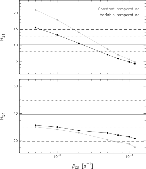
Figure 13: Modelled flux ratios $R$ as a function of CS photodissociation rate for CS $J$(2–1) ($R_{21}$, top) and $J$(5–4) ($R_{54}$, bottom) lines for $\beta_{\rm CS_{2}}$ = 1.7 $\times$ 10^-3 s^-1 (value at $r_{h}$ = 1 AU). The dotted (respectively dashed) lines show the 1-$\sigma$ (resp. 2-$\sigma$) range around the observed value (continuous line).

Figure 14: Amplitude of the visibility as a function of $uv$-radius for CS $J$(2–1) (upper panel) and CS $J$(5–4) (lower panel). Measurements are shown by dots with error bars. Displayed modelled visibilities are for a variable temperature law and parameter sets: ($\beta_{\rm CS}$ = 2 $\times$ 10^-5 s^-1, $\beta_{\rm CS_{2}}$ = 1.7 $\times$ 10^-3 s^-1) in solid line, ($\beta_{\rm CS}$ = 2 $\times$ 10^-5 s^-1, $\beta_{\rm CS_{2}}$ = 1 $\times$ 10^-3 s^-1) in dashed line and ($\beta_{\rm CS}$ = 1 $\times$ 10^-4 s^-1, $\beta_{\rm CS_{2}}$ = 1.7 $\times$ 10^-3 s^-1) in dotted line.

Ultraviolet observations of CS performed with the International Ultraviolet Explorer (IUE) have shown that CS₂ is the likely parent of CS (Jackson et al. 1982, 1986). More recently, a comparison between unidentified lines in comet 122P/de Vico spectra and jet cooled laboratory CS₂ spectra suggests that CS₂ is indeed present in cometary atmospheres (Jackson et al. 2004). The CS₂ lifetime at 1 AU is estimated between 590 s (Jackson et al. 1986) and 1000 s (Feldman et al. 1999) from observations and laboratory measurements (i.e., photodissociation rate $\beta_{\rm CS_{2}}$ between 1 and 1.7 $\times$ 10^-3 s^-1).

The photodissociation rate of CS is debated. From IUE observations, Jackson et al. (1982) deduced $\beta_{\rm CS}$ = 1 $\times$ 10^-5 s^-1. From CS $J$(2–1) interferometric observations of comet Hale-Bopp performed with the BIMA array, Snyder et al. (2001) inferred $\beta_{\rm CS}$ = 1 $\times$ 10^-4 s^-1, i.e. a value ten times higher. On the other hand, single-dish millimetric observations of comets at small heliocentric distances suggested $\beta_{\rm CS}\approx 2\times 10^{-5}$ s^-1 (Biver et al. 2003).

The field of view radius of our CS ON–OFF observations is 10000 to 25000 km, depending on the line (Table 1). Therefore, the calculated flux ratio $F_{\rm SD}$ and $F_{\rm Int}$ should be strongly dependent upon the assumed CS scalelength, when exploring values between 10000 and 100000 km. On the other hand, the interferometric beams (750 to 2000 km radius, for the $J$(5–4) and $J$(2–1) lines, respectively) are comparable to the CS₂ scalelength, which makes the determination of the CS₂ lifetime more difficult, given large uncertainties in CS lifetime.

Figure 13 shows the dependence of the flux ratio of the $J$(2–1) ($R_{21}$) and $J$(5–4) ($R_{54}$) lines with the photodissociation rate of CS, assuming a constant or a variable temperature in the coma. The CS₂ photodissociation rate was taken equal to $\beta_{\rm CS_{2}}$ = 1.7 $\times$ 10^-3 s^-1 (value at $r_{h}$ = 1 AU). The observed ratios can be reproduced within 2-$\sigma$, with $\beta_{CS}$ in the range 2–7 $\times$ 10^-5 s^-1 (case of constant $T$) or with $\beta_{CS}$ between 0.7 and 6 $\times$ 10^-5 s^-1 (case of variable $T$). The same computations were made with $\beta_{\rm CS_{2}}$ = 1 $\times$ 10^-3 s^-1 (Feldman et al. 1999) in order to investigate the sensitivity of the results to this parameter. A satisfactory fit within 1-$\sigma$ is obtained for both lines ($R_{21}$ = 12 and $R_{54}$ = 29) with $\beta_{\rm CS}$ in the range 2–5 $\times$ 10^-5 s^-1 and a variable $T$. In summary, our data are consistent with a CS photodissociation rate of 1–5 $\times$ 10^-5 s^-1. On the basis of the $J$(2–1) data alone, the value $\beta_{\rm CS}$ = 2–3 $\times$ 10^-5 s^-1 is preferred. Models assuming a variable temperature in the coma provide the best results.

Table 6 shows that opacity effects strongly affect the intensity of the $J$(5–4) line in the interferometric beam, justifying our radiative transfer model. They are less significant for $J$(2–1), and for $T$ = 120 K than for variable $T$. These trends can be easily explained: 1) the $J$(5–4) is intrinsically stronger and observed with a smaller field of view; 2) with the adopted variable temperature law, the lower rotational levels of the $J$(2–1) and $J$(5–4) transitions (namely $J$ = 1 and $J$ = 4) are more significantly populated in the inner coma (see Fig. 10), hence more significant self-absorption effects. The retrieved CS production rate is $\sim$ 2 $\times$ 10²⁸ s^-1 with $\beta_{\rm CS}$ = 1–2 $\times$ 10^-5 s^-1.

In Fig. 14 we show the radial evolution of the visibilities for different model parameters, assuming a variable temperature in the coma. Models with $\beta_{\rm CS}$ = 2 $\times$ 10^-5 s^-1 and $\beta_{\rm CS_{2}}$ equal to 1 $\times$ 10^-3 s^-1 and 1.7 $\times$ 10^-3 s^-1 reproduce correctly the observed visibilities, as expected from the study of the fluxes ratio. Visibilities computed with $\beta_{\rm CS}$ = 1 $\times$ 10^-4 s^-1 do not match the data.

The high value $\beta_{\rm CS}=1\times 10^{-4}\,\textrm{s}^{-1}$ inferred by Snyder et al. (2001) from comet Hale-Bopp observations of CS $J$(2–1) with the BIMA array is ruled out by our analysis of Plateau de Bure observations. Snyder et al. (2001) used a different approach. They analysed CS radial profiles deduced from the interferometric maps, but did not consider the autocorrelation measurements that they acquired nor the radial evolution of the visibilities in the $uv$–plane. However, for $\beta_{\rm CS}=1\times 10^{-4}\,\textrm{s}^{-1}$, their autocorrelation data yield systematically higher (by a factor 2.5–3) CS production rates than the cross-correlation data. We computed that, if $\beta_{\rm CS}$ is decreased to $\sim 3\times 10^{-5}\,\textrm{s}^{-1}$, the production rates derived by the two sets of data can be reconciled.

5.3 Sulfur monoxide SO

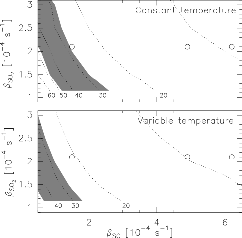
Figure 15: The flux ratio $R=\frac{F_{\rm SD}}{F_{\rm Int}}$ as a function of $\beta_{SO}$ and $\beta_{SO_{2}}$. Upper panel: for constant temperature $T$ = 120 K; lower panel: for the variable temperature law. Contour values are given in the bottom of the figures. Circles correspond to ($\beta_{SO}$, $\beta_{SO_{2}}$) values published in the literature (Table 5). The region where the computed $R$ is in agreement within 1-$\sigma$ with the observations ($R=38\pm 10$) is filled in grey.

As pointed out in Sect. 2.3.2, there is clear evidence that the SO radial brightness distribution is much more extended than that of H₂S. The flux ratio for the SO line is $R=38\pm 10$, taking into account calibration uncertainties, to be compared to $R=5.4\pm 1.2$ for the H₂S line (Table 6). SO is a radical and a photodissociation product of SO₂, also observed in comet Hale-Bopp (Bockelée-Morvan et al. 2000). Published SO₂ photodissociation rates are in general consistent with each other: $\beta_{\rm SO_{2}}=2.1-2.3\times 10^{-4}\,\mathrm{s}^{-1}$ for quiet sun and $2.9\times 10^{-4}\,\mathrm{s}^{-1}$ for active sun (see Table 5). A significantly lower value was derived by Kumar (1982), but only one channel of the SO₂ photodissociation process was considered. We will not consider this value in this work.

In contrast, published values of $\beta_{\rm SO}$ differ by up to a factor of 4 (Table 5). Because SO and $\textrm{SO}_{2}$ photodissociative scalelengths are intermediate between the primary and interferometric fields of view, they can be somewhat constrained by the observations. Model calculations were performed for many couples ($\beta_{\rm SO}$, $\beta_{\rm SO_{2}}$) in the range of published values. Isocontours of the flux ratio $R$ as a function of $\beta_{\rm SO}$ and $\beta_{\rm SO_{2}}$ are presented in Fig. 15.

In the assumption that SO is produced solely by the photodissociation of $\textrm{SO}_{2}$, the observations are consistent (within 1–1.5-$\sigma$) with the published value of $\beta_{\rm SO}=1.5\times 10^{-4}\,\mathrm{s}^{-1}$ (Kim & A’Hearn 1991), but are not compatible with values as high as $5-6\times 10^{-4}\,\mathrm{s}^{-1}$ (Huebner et al., 1992; Summers & Strobel, 1996). The same conclusion is obtained from the study of the visibility curve (Fig. 16). Direct release of SO from the nucleus is fully excluded (Fig. 16).

Published $\beta_{\rm SO}$ rates are all based on the same laboratory data (Phillips, 1981). Discrepancies may be ascribed to the complexity of the laboratory SO absorption spectrum (which shows a series of strong narrow lines over a broad continuum) and the fact that the spectrum is only available in a graphic version. From our own analysis of the spectrum, we put a firm lower limit $\beta_{\rm SO}$ $>1.5\times 10^{-4}\,\mathrm{s}^{-1}$ using the lower envelope to the SO spectrum. Considering in addition the narrow lines, we estimate $\beta_{\rm SO}$ = $3.2\times 10^{-4}\,\mathrm{s}^{-1}$, but this estimation is still uncertain due to the lack of a digital version of the spectrum.

How this result could be reconciled with our measurements? First, because SO emission is strongly anisotropic, can we exclude a flaw in our analysis due to simple approximations made on the coma structure? Calculations performed for an anisotropic coma which reproduces the main characteristics of the SO map (Sect.2.3.2) show that our analysis should not be significantly affected by the presence of jets in the coma. In addition, a separate reduction of the blue and red velocity parts of the SO spectrum shows that both parts display the same intensity flux ratio $R$ (equal to that measured for the whole emission), indicating that jet structures do not affect the overall evolution of the visibilities with baseline length.

A $\beta_{\rm SO}$ value higher than that which fits the observations implies that some process makes the SO brightness radial distribution more extended than expected from SO₂ photodissociation. We examined several possibilities. Among those that can be excluded are: 1) a $\beta_{\rm SO_{2}}$ value lower than published values; shielding of SO₂ photodissociation by water is insufficient (the inner coma where UV shielding by water is significant may be evaluated to $r<1000$ km); 2) a kinetic temperature that is much higher ( $\sim$ 200 K) in the inner coma observed by the interferometric beam than in the outer coma observed by the primary beam, that would be in contradiction with measurements (Magee-Sauer et al., 1999; DiSanti et al., 2001) and hydrodynamical models (Combi et al., 1999). This leaves the possibility that SO₂ is not the only source of SO, or that SO₂ is itself produced by some extended source in the coma such as grains or complex molecules.

The SO production rate deduced from the observations is 2.4–2.7 $\times$ 10²⁸ s^-1 for $\beta_{\rm SO}=1.5\times 10^{-4}\,\mathrm{s}^{-1}$ and $\beta_{\rm SO_{2}}=2.1\times 10^{-4}\,\mathrm{s}^{-1}$. Based on the same ON–OFF data, Bockelée-Morvan et al. (2000) inferred a higher value for the SO production rate due to different assumptions on the beam efficiency and kinetic temperature. SO₂ was observed in comet Hale-Bopp on several dates in March and April 1997 using the IRAM Plateau de Bure and 30-m antennas (Bockelée-Morvan et al. 2000). The measurements yield a production ratio $Q_{\rm SO}$/$Q_{\rm SO_{2}}\sim 2$ in March 1997. The discrepancy increases when a higher $\beta_{\rm SO}$ value is adopted (e.g., $Q_{\rm SO}$/$Q_{\rm SO_{2}}\sim 6$ for $\beta_{\rm SO}=6.2\times 10^{-4}\,\mathrm{s}^{-1}$). Bockelée-Morvan et al. (2000) suggest that $Q_{\rm SO_{2}}$ is possibly underestimated in their calculations as they assumed LTE for the SO₂ rotational population distribution, and neglect electronic and vibrational excitation. Another possible explanation is the presence of another source of SO in the coma. As discussed above, this would allow a more satisfactory interpretation of the observed SO radial distribution, given available estimations of $\beta_{\rm SO}$.

The synthetic SO ON–OFF spectrum computed with our isotropic model is plotted in Fig. 3. Though it does not match in details the observed asymmetric SO spectrum, the line width and wings are correctly reproduced. This indicates that, as assumed in the model, the SO radicals which are within the field of view, though daughter products, do indeed partake in the kinetics of the gas flow.

Figure 16: Amplitude of visibility of SO 220 GHz line versus $uv$-radius. Observations: circles with error bars. Continuous, dotted and dashed lines correspond to model calculations assuming that SO is created by the photodissociation of SO₂ with $\beta_{SO}$ of 1.5, 4.9 and $6.2\times 10^{-4}\,\mathrm{s}^{-1}$, respectively. The dotted-dashed line tests the case of a pure nuclear origin for SO, with $\beta_{SO}=1.5\times 10^{-4}\,\mathrm{s}^{-1}$. Calculations correspond to variable $T$ law. Similar results are obtained with a constant $T$ = 120 K.

6 Summary

Observations carried out in cross- and autocorrelation modes with the IRAM Plateau de Bure interferometer were analysed to study the spatial distribution of sulfur-bearing molecules in the coma of comet Hale-Bopp using a radiative transfer code. The radial distribution of H₂S is in agreement with a direct release from the nucleus and is well reproduced by our model using the H₂S photodissociation rate published in the literature, thereby validating our approach.

On this basis, we studied the radial distribution of CS emission. This radical is believed to be produced by the photolysis of the short-lived CS₂ molecule. The angular resolution of the observations prevented us to obtain observational constraints on the CS₂ photodissociation rate. The photodissociation rate of CS is not precisely determined because no satisfactory measurements can be done in the laboratory on this radical. Our data are consistent with $\beta_{CS}$ in the range $1-5\times 10^{-5}\,\mathrm{s}^{-1}$, which is in agreement with the value of $2\times 10^{-5}\,\mathrm{s}^{-1}$ proposed by Biver et al. (2003) but rules out $\beta_{CS}=1\times 10^{-4}\,\mathrm{s}^{-1}$ derived by Snyder et al. (2001) from interferometric observations with the BIMA array. With $\beta_{CS}\sim 3\times 10^{-5}\,\mathrm{s}^{-1}$, the CS production rates derived from autocorrelation and cross-correlation BIMA data are reconciled.

SO was first detected in comet Hale-Bopp, as well as its presumed parent product SO₂ (Bockelée-Morvan et al., 2000). Values of $\beta_{SO}$ available in the literature differ by a factor of $\sim$4 between the lowest ($1.5\times 10^{-4}\,\mathrm{s}^{-1}$, Kim & A’Hearn 1991) and the highest value ($6.2\times 10^{-4}\,\mathrm{s}^{-1}$, Huebner et al. 1992). From our own analysis based on the same laboratory absorption spectrum, we estimate $\beta_{SO}\sim 3.2\times 10^{-4}\,\mathrm{s}^{-1}$. In contrast, assuming that SO₂ is the parent of SO, the SO interferometric data suggest $\beta_{SO}$ $=1.5\times 10^{-4}\,\mathrm{s}^{-1}$. The discrepancy between measured and computed values of the SO photodissociation rate may indicate that SO₂ is not the sole parent of SO, or that SO₂ is itself created by some extended source in the coma. Note that the sulfur chemistry in comets is far from being fully understood: the origins of S₂ and NS radicals are still unknown (Bockelée-Morvan et al., 2004). In the future, interferometric mapping of SO and SO₂ with the Atacama Large Millimeter and submillimeter Array (ALMA) will provide relevant informations about the SO creation process in cometary atmospheres (Biver 2005). Further laboratory experiments on SO absorption in the UV are also strongly encouraged.

The data show clear evidence for anisotropic spatial distributions in the coma: (1) ON–OFF spectra are asymmetric; (2) the visibilities as a function of $uv$-radius do not follow the expected curves in the case of a 1-D outflow ; (3) maps of CS and SO line brightness distributions do not peak at the position of the continuum maps obtained simultaneously which should be close to the nucleus position; (4) maps show strong and specific spectral variations in the coma. On the basis of model calculations, we show that SO and CS present a wide jet-like structure that may correspond to the gaseous counterpart of the strong high latitude dust jet detected at optical wavelengths. This structure is not observed for H₂S. All three molecules show day/night spatial asymmetries. Spectral temporal variations related to nucleus rotation are only observed for CS. The strong CO rotating jet observed at Plateau de Bure interferometer has no H₂S, CS and SO counterpart. These differences in the outgassing patterns of different volatiles in the Hale-Bopp coma may suggest that the nucleus composition is inhomogeneous (though all molecules were not observed on the same day and we cannot exclude time variations of the outgassing). This analysis is consistent with the results of some previous works: (1) the offsets observed between molecular (HNC, DCN, HDO) and continuum emission on interferometric maps made with the Owens Valley Radio Observatory (OVRO) were interpreted as due to jets enriched in these molecules (Blake et al., 1999); (2) Monte Carlo simulations suggest that the different molecular jets observed at optical wavelengths (OH, CN, C₂) originate in several active areas of different chemical compositions (Lederer et al., 2002). An explanation would be that the huge nucleus of comet Hale-Bopp is actually made of several pieces that have not undergone the same formation and/or evolution processes. This would be in contrast with comet 73P/Schwassmann-Wachmann 3 whose fragments were found similar in chemical properties, suggesting an homogeneous nucleus (Dello Russo et al., 2007).

The results obtained in this paper demonstrate the benefit and uniqueness of millimeter interferometry to investigate nucleus outgassing properties and physical processes acting in the coma. Last and not least, by solving the contentious issue regarding the role of nongravitational forces in comet Hale-Bopp orbit, we have shown that this technique is also powerful for astrometry purposes. ALMA, with its unprecedented sensitivity, angular resolution, and instantaneous $uv$-coverage, will be a very powerful tool in the future for cometary science.