Spinflation and Cycling Branes
in Warped Throats

Abstract

The implications of brane motion in angular directions of Calabi-Yau flux compactifications are discussed from the point of view of an observer living on the worldvolume of the brane and from the point of view of an observer living elsewhere in the three non-compact dimensions. The brane observer can experience cosmological bounces and cyclic behavior of the scale factor induced by centrifugal angular momentum barriers. Observers living elsewhere in the compactification experience marginally prolonged periods of inflation due to large angular momentum (spinflation). The presence of spinflaton fields (or other fields with non-standard kinetic terms) during inflation may lead to interesting observational signatures in the cosmic microwave background radiation.

1 Introduction

The most well studied constructions of brane inflation in string theory are within the context of orientifolds of Calabi-Yau flux compactifications of Type IIB superstring theory.  In these constructions it is possible to stabilize all phenomenologically dangerous moduli (complex structure and dilaton as well as Kähler moduli). The stabilization involves both fluxes threading cycles of the Calabi-Yau and non-perturbative elements such as D7-branes (or Euclidean D3-brane instantons) wrapping four-cycles  Giddings:2001yu ; Kachru:2003aw . The fluxes can produce a large warped throat region providing a relatively stable and concrete setting for the study of brane dynamics. We consider the motion of a D3-brane probe in this throat both from the point of view of an observer on the brane and from the point of view of an observer living elsewhere (somewhere in the compactification where the Standard Model can be embedded). In addition to examining radial motion of the brane we allow the brane to move with angular momentum in the extra dimensions.

2 Cycling branes and angular momentum

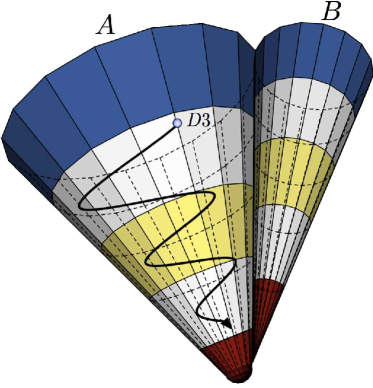
Figure 1: The warped deformed conifold and spinning D3-brane probe. The dual $A$ and $B$ cycles decrease in size from the ultraviolet to the infrared where they end in a smooth $S^{3}$ and zero size $S^{2}$, respectively. The geometry is composed of $N$ D3 and $M$ D5-branes.

In general, Calabi-Yau spaces are nonsingular; however, for certain values of parameters they can develop singularities. Locally these singularities appear as a cone, or “conifold”. When fluxes are introduced this cone can become a warped throat region. Here we take this throat to be the nonsingular warped deformed conifold (or Klebanov-Strassler (KS) geometry) Klebanov:2000hb .  Far from the tip the space is approximated by the conifold $T^{(1,1)}=S^{2}\times S^{3}$ (topologically an $S^{2}$ fibered over an $S^{3}$). In Calabi-Yau manifolds three-cycles come in Poincaré duals. The throat decomposes into two such three-cycles, the $A$ and dual $B$ cycle. The geometry is supported by $N$ D3-branes and $M$ D5-branes wrapping the $S^{2}$ of $T^{(1,1)}$ (so-called fractional D3-branes). The background fluxes are composed of both the RR and NS-NS three-forms present in Type IIB superstring theory and thread the $A$ and $B$ cycles respectively:

$$\int_{A}F_{3}\sim M\,,\qquad\int_{B}H_{3}\sim-K\,,$$ (1)

where $K=N/M$.

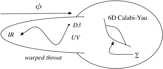
Figure 2: Sketch of Calabi-Yau flux compactification with warped throat region. The position of the D3-brane in the throat is parameterized by $\phi$ and $\Sigma$ is a four-cycle. There are wrapped D-branes and orientifold planes not included in this diagram.

The $A$ cycle ends in a smooth $S^{3}$ (see Figure 1). The fluxes stabilize the dilaton and complex structure (shape) moduli but do not lift the closed string Kähler moduli associated with the volumes of four-cycles in the compactification Giddings:2001yu . This stabilization is accomplished by nonperturbative effects such as D7-branes wrapped around the four-cycles $\Sigma_{4}^{(i)}$ in the space Kachru:2003aw . The KS throat is smoothly glued onto the Calabi-Yau space in the ultraviolet (UV) (see Figure 2).

Consider the dynamics of a D3-brane probe in this background. The D3 brane fills four-dimensional spacetime $\{t,x^{1},x^{2},x^{3}\}$ and appears point-like in the internal space. The metric ansatz is:

$$ds_{10}^{2}\,=\,h^{-1/2}\,g_{\mu\nu}dx^{\mu}dx^{\nu}\,+\,h^{1/2}\,{\rm g}_{mn}dy^{m}dy^{n}\,,$$ (2)

where $h$ is the warp factor, $g_{\mu\nu}$ is the metric in four-dimensions and ${\rm g}_{mn}$ is the metric of the internal space.

The location of the brane in the extra dimensions is parameterized by a field $\phi$. This field is related to the proper radial throat coordinate $r$ (the proper length with respect to the internal metric (i.e. ${\rm g}_{rr}=1$)) by $\phi=\sqrt{T_{3}}r$, where $T_{3}$ is the brane tension given in terms of the string length, $\alpha^{\prime}=\ell_{s}^{2}$, by $T_{3}=((2\pi)^{3}\alpha^{\prime 2})^{-1}$. In principle the brane is free to move in the five angular coordinates $y^{s}=\{\psi,\phi_{1},\phi_{2},\theta_{1},\theta_{2}\}$. It is the motion in these angular coordinates that is usually ignored and that we focus on here.

The brane motion is described by the Dirac-Born-Infeld (DBI) action plus Wess-Zumino term:

$$S=-T_{3}g_{s}^{-1}\int{d^{4}x\,h^{-1}\left[e^{-3\varphi}\,\sqrt{1-h\,v^{2}}-1\right]}\,,$$ (3)

where $g_{s}$ is the string coupling, $\varphi$ is the dilaton and $v^{2}=g_{mn}\dot{y}^{m}\dot{y}^{n}$. The warp factor of the KS geometry is:

$$h(\eta)=(g_{s}M\alpha^{\prime})^{2}2^{2/3}\,\zeta^{-8/3}\int_{\eta}^{\infty}{dx\,\frac{x\,\coth{x}-1}{\sinh^{2}{x}}\,\left(\sinh{(2\,x)-2\,x}\right)^{1/3}}\,.$$ (4)

Here $\zeta$ is a dimension-full parameter, $[\zeta^{2/3}]=\ell$, and $\eta$ is the dimensionless geometric coordinate parameterizing the throat. The geometric variable is related to the radial coordinate via the transformation:

$$r=\frac{\zeta^{2/3}}{\sqrt{6}}\int_{0}^{\eta}\frac{\sinh x\,dx}{(\sinh x\,\cosh x-x)^{1/3}}\,.$$ (5)

A tedious calculation yields the surprisingly simple result for the ten-dimensional Ricci curvature of the KS space:

$$R=-\frac{4h^{\prime}(\eta)+3h^{\prime\prime}(\eta)(\coth{\eta}-\eta\,\mbox{csch}^{2}{\eta})}{\zeta^{4/3}h(\eta)^{3/2}(\cosh{\eta}\sinh{\eta}-\eta)^{1/3}}\,.$$ (6)

As an illustrative example, we allow the brane to move in the radial $\eta$ direction and in the angular $\psi$ and $\theta_{1}$ directions:

$$v^{2}=A(\eta)\,\left[\dot{\eta}^{2}+\dot{\psi}^{2}\right]+B(\eta)\,\dot{\theta}_{1}^{2}\,,$$ (7)

where

$$A(\eta)=\frac{\zeta^{4/3}}{6K^{2}}\,,\qquad\quad B(\eta)=\frac{\zeta^{4/3}K}{4}\,\left[\cosh^{2}{(\eta/2)}+\sinh^{2}{(\eta/2)}\right]$$ (8)

and

$$K(\eta)=\frac{\left(\sinh{(2\,\eta)-2\,\eta}\right)^{1/3}}{2^{1/3}\,\sinh{\eta}}\,.$$ (9)

In general, the conserved angular momenta are given by:

$$\ell_{r}=\frac{g_{rs}\dot{y}^{2}}{\sqrt{1-hv^{2}}}\,,$$ (10)

corresponding to the conserved q-numbers of the symmetry group. The conserved angular momenta in our example are $l_{\psi}=\frac{A\,\dot{\psi}}{\sqrt{1-h\,v^{2}}}$, $l_{\theta_{1}}=\frac{B\,\dot{\theta}_{1}}{\sqrt{1-h\,v^{2}}}$, and the conserved energy (per unit mass) is

$$\epsilon=\frac{1}{h}\left[\sqrt{\frac{1+h\,\ell^{2}(\eta)}{1-h\,g_{\eta\eta}\,\dot{\eta}^{2}}}-q\right]$$ (11)

where $\ell^{2}(\eta)=\frac{l_{\psi}^{2}}{A}+\frac{l_{\theta_{1}}^{2}}{B}\,.$ The time evolution of the radial coordinate $\eta$ is

$$\dot{\eta}^{2}=\frac{\left[\varepsilon(h\,\varepsilon+2)-\ell^{2}(\eta)\right]}{A(h\,\varepsilon+1)^{2}}=Q\,.$$ (12)

The zeros of $Q$ determine turning (bounce) points in the brane trajectory. We plot $Q(\eta)$ for typical values of the parameters in Figure 3.

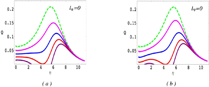
Figure 3: The function $Q$ for a brane moving in the KS background as the angular momenta is increased from $0$ (top, dashed line) to higher values. In $(a)$ we keep $l_{\theta_{1}}=0$, and allow $l_{\psi}$ to vary, whereas in $(b)$ we keep $l_{\psi}=0$ and change $l_{\theta_{1}}$. The zeros of $Q$ correspond to turning points in the brane trajectory.

2.1 Induced bouncing and cyclic cosmologies

An observer living on the D3-brane experiences expansion and contraction depending on the motion of the brane in the warped throat. The projected metric in four dimensions may be written in Friedmann-Robertson-Walker (FRW) form:

$$ds^{2}=h^{-1/2}\left(-(1-h\,v^{2})\,dt^{2}+dx_{i}dx^{i}\right)=-d\tau^{2}+a^{2}(\tau)dx_{i}dx^{i}\,,$$ (13)

with scale factor

$$a(\tau)=h^{-1/4}(\eta(\tau))$$ (14)

and with brane cosmic time related to the bulk time coordinate by

$$d\tau=h^{-1/4}\sqrt{(1-h\,v^{2})}\,dt\,.$$ (15)

The resulting expansion on the brane is induced by the warping of the background as in Easson:2007fz ; Kehagias:1999vr ; Kachru:2002kx ; sling . From Figure 3, it is clear that the brane observer can experience bounces in the scale factor $a(\tau)$ either when the brane reaches the end of the smooth KS geometry or when a bounce occurs due to large angular momentum (zeros of $Q$). When the brane moves down the throat the brane scale factor contracts and when the brane moves up the throat it expands. The expansion and contraction rate is determined by the warp factor in the throat, $h$, and is quantified by the Hubble parameter $H=a^{-1}da/d\tau$. The lowermost solution in Figure 3 (b) is a bound state where the brane bounces back and forth between two zeros of $Q$. This corresponds to a cyclic cosmology from the brane observer’s point of view.

The above models provide interesting string theory motivated, time-dependent solutions that yield bounces and cyclic motion in the scale factor. They therefore provide testing grounds for discovering general physical features more realistic cyclic and bouncing cosmologies may posses. There are serious challenges, however, for a cosmological scenario based on the mirage picture to overcome. For example, because the cosmological expansion is induced by the background warping, it is unclear how to reheat the Universe or recover Einstein gravity on the brane at late times Kachru:2002kx ; Linde:2007fr . Furthermore, mirage cosmology branes bouncing through the tip of KS typically have an unacceptably large blue tilt to the scalar spectral index, $n_{s}$, on super-Hubble scales in the expanding phase Brandenberger:2007by .

2.2 Spinflation

Alternative to the mirage picture, one may study cosmological dynamics from the perspective of an observer living elsewhere in the Calabi-Yau (e.g. on a stack of $\mathcal{N}$ D3-branes) spin . In this case the motion of the D3-brane in the throat gives rise to an inflaton field $\phi$ (related to the geometric radial coordinate $\eta$) in the four-dimensional effective theory of the elsewhere observer Kachru:2003sx . If the brane is spinning, the conserved angular momentum may appear as a field (or several fields, $\phi_{m}$) in the effective theory obtained by integrating out the internal coordinates:

$$S = \frac{M_{Pl}^{2}}{2}\int{d^{4}x\sqrt{-g}\,R}$$ (16)

$$-\,g_{s}^{-1}\int{d^{4}x\sqrt{-g}\left[f^{-1}\sqrt{1+f\,g_{mn}g^{\mu\nu}\partial_{\mu}\phi^{m}\partial_{\nu}\phi^{n}}-q\,f^{-1}+V(\phi^{m})\right]}\,,$$

where the field theory function $f(\phi)$ is related to the warp factor $h(r)$ by $f(\phi)=T_{3}^{-1}h(\phi/\sqrt{T_{3}})$. The four-dimensional Einstein-Hilbert action arises from dimensional reduction of the closed string sector of the ten-dimensional action st . The fluctuations of the brane are described by the Dirac-Born-Infeld action. The Planck mass, $M_{Pl}$ is relate to the internal six-dimensional volume, $V_{6}$, by $M_{Pl}^{2}=V_{6}/\kappa^{2}_{10}$, where $\kappa_{10}^{2}=(2\pi)^{7}g_{s}^{2}\alpha^{\prime 4}$. The potential $V$ generally arises once the system is coupled to other sectors of the theory. In a realistic model the potential can be quite complicated, however, for our purposes it suffices to consider the simple $m^{2}\phi^{2}$ potential.

Assuming an FRW ansatz for the metric and defining $\beta=(3\,g_{s}\,M_{Pl}^{2})^{-1}$, the equations of motion can be written

$$fg_{\phi\phi}\,\dot{\phi}^{2} = 1-\left(1+\frac{f\ell^{2}(\phi)}{a^{6}}\right)\cdot\left(1+f\left(\frac{H^{2}}{\beta}-V\right)\right)^{-2}$$ (17)

$$\dot{H} = -\frac{3\beta}{2}\left[2\left(\frac{H^{2}}{\beta}-V\right)+f\left(\frac{H^{2}}{\beta}-V\right)^{2}\right]\cdot\left(1+f\left(\frac{H^{2}}{\beta}-V\right)\right)^{-1}\,,$$ (18)

subject to the Friedmann constraint

$$H^{2}=\beta\left(\frac{1}{f}\left[\gamma-1\right]+V\right)\,,$$ (19)

where we have defined the Hubble parameter $H\equiv\dot{a}/a$ and angular momentum $\ell^{2}(\phi)=g^{rs}\,l_{r}l_{s}$, $l_{m}\equiv a^{3}\,g_{mn}\,\dot{\theta}^{n}\gamma$ and $\gamma$ is the “lorentz” factor generated by the non-standard kinetic term for the fields in (16):

$$\gamma\,=\,\sqrt{\frac{1+f\,\ell^{2}(\phi)/a^{6}}{1-f\,g_{\phi\phi}\,\dot{\phi}^{2}}}\,.$$ (20)

Equation (20) places an upper bound on the brane velocity in the radial direction: $|\dot{\phi}|<\sqrt{f^{-1}}$. The velocity bound operates independently from the presence of angular momentum and leads to inflation in models with potentials normally too steep to do so st . It would appear, however, that it is difficult to build a successful model of DBI inflation in the KS geometry, as $\gamma$ seemingly grows too large to ignore back reaction effects of the probe brane spin .

From the point of view of the elsewhere observer and in contrast to the brane-bound observer the D3-brane inflaton always drives expansion of the four-dimensional scale factor $a(t)$. The brane probe bounces up and down through the tip of the KS throat leading to inflation sourced by the DBI action (16). The bounces are strongly damped by the force due to the potential $V$. If the inflaton couples to standard model fields (e.g. through couplings of the form $g^{2}\phi^{2}\xi^{2}$ or $h\phi\bar{\psi}\psi$) reheating will occur Brodie:2003qv .

The addition of angular momentum alters the form of the acceleration parameter:

$$\varepsilon\,\equiv\,-\frac{\dot{H}}{H^{2}}\,.$$ (21)

Using equations (17) and (18) we have:

$$\varepsilon\,=\,\frac{3\beta}{2H^{2}}\left\{\left[1+f\left(\frac{3H^{2}}{\beta}-V\right)\right]\,\dot{\phi}^{2}+\frac{l^{2}(\phi)}{a^{6}}\left[1+f\left(\frac{3H^{2}}{\beta}-V\right)\right]^{-1}\right\}\,.$$ (22)

Although the angular momentum term adds a positive contribution to $\epsilon$, its dominant effect is to decrease the overall value of $\epsilon$ by decreasing the brane speed $\dot{\phi}$. Hence, the addition of angular momentum tends to prolong the inflationary period by allowing the acceleration parameter to remain small for a slightly longer period of time. The angular momentum is suppressed by $a^{-6}$ and is therefore rapidly diluted during inflation; however, spinflaton fields can help a given inflationary scenario by providing a small number of extra e-foldings of expansion at early times.

It would be interesting to look for observable signatures of spinflaton fields, for example, in the cosmic microwave background radiation. Such a search requires an understanding of cosmological perturbation theory in multi-field models with non-standard kinetic terms. We have initiated this study in spin . We found the distinctive feature that non-adiabatic entropy modes and adiabatic curvature perturbations propagate with different speeds. This leads to a suppression in the conversion of isocurvature to curvature perturbations and unique observable features in the form of non-gaussianities bret , above and beyond the familiar non-gaussianities associated with DBI inflation ast .

References

- (1) G. R. Dvali and S. H. H. Tye, Phys. Lett. B 450, 72 (1999) [arXiv:hep-ph/9812483].
- (2) S. H. S. Alexander, Phys. Rev. D 65, 023507 (2002) [arXiv:hep-th/0105032].
- (3) G. R. Dvali, Q. Shafi and S. Solganik, arXiv:hep-th/0105203.
- (4) C. P. Burgess, M. Majumdar, D. Nolte, F. Quevedo, G. Rajesh and R. J. Zhang, JHEP 0107, 047 (2001) [arXiv:hep-th/0105204].
- (5) J. H. Brodie and D. A. Easson, JCAP 0312, 004 (2003) [arXiv:hep-th/0301138].
- (6) S. Kachru, R. Kallosh, A. Linde, J. M. Maldacena, L. McAllister and S. P. Trivedi, JCAP 0310, 013 (2003) [arXiv:hep-th/0308055].
- (7) S. B. Giddings, S. Kachru and J. Polchinski, Phys. Rev. D 66, 106006 (2002) [arXiv:hep-th/0105097].
- (8) S. Kachru, R. Kallosh, A. Linde and S. P. Trivedi, Phys. Rev. D 68, 046005 (2003) [arXiv:hep-th/0301240].
- (9) I. R. Klebanov and M. J. Strassler, JHEP 0008, 052 (2000) [arXiv:hep-th/0007191].
- (10) D. Easson, R. Gregory, G. Tasinato and I. Zavala, JHEP 0704, 026 (2007) [arXiv:hep-th/0701252].
- (11) A. Kehagias and E. Kiritsis, JHEP 9911, 022 (1999) [arXiv:hep-th/9910174].
- (12) S. Kachru and L. McAllister, JHEP 0303, 018 (2003) [arXiv:hep-th/0205209].
- (13) C. Germani, N. E. Grandi and A. Kehagias, arXiv:hep-th/0611246.
- (14) A. Linde, arXiv:0705.0164 [hep-th].
- (15) R. Brandenberger, H. Firouzjahi and O. Saremi, arXiv:0707.4181 [hep-th].
- (16) D. A. Easson, R. Gregory, D. F. Mota, G. Tasinato and I. Zavala, arXiv:0709.2666 [hep-th].
- (17) E. Silverstein and D. Tong, Phys. Rev. D 70, 103505 (2004) [arXiv:hep-th/0310221].
- (18) M. x. Huang, G. Shiu and B. Underwood, arXiv:0709.3299 [hep-th].
- (19) M. Alishahiha, E. Silverstein and D. Tong, Phys. Rev. D 70, 123505 (2004) [arXiv:hep-th/0404084].