Numerical simulations of type III planetary migration:
II. Inward migration of massive planets

Abstract

We present a numerical study of rapid, so called type III migration for Jupiter-sized planets embedded in a protoplanetary disc. We limit ourselves to the case of inward migration, and study in detail its evolution and physics, concentrating on the structure of the corotation and circumplanetary regions, and processes for stopping migration. We also consider the dependence of the migration behaviour on several key parameters. We perform this study using the results of global, two-dimensional hydrodynamical simulations with adaptive mesh refinement. The initial conditions are chosen to satisfy the condition for rapid inward migration. We find that type III migration can be divided into two regimes, fast and slow. The structure of the co-orbital region, mass accumulation rate, and migration behaviour differ between these two regimes. All our simulations show a transition from the fast to the slow regime, ending type III migration well before reaching the star. The stopping radius is found to be larger for more massive planets and less massive discs. A sharp density drop is also found to be an efficient stopping mechanism. In the fast migration limit the migration rate and induced eccentricity are lower for less massive discs, but almost do not depend on planet mass. Eccentricity is damped on the migration time scale.

1 Introduction

The theory of disk-planet interaction aims at finding a physical description of the gravitational interaction between gas-dust protoplanetary disks and protoplanets. A major advance, in comparison with the theories of solar system formation from 20 years ago, was the realization that protoplanets can globally migrate and consequently that planets can be found on orbits different from the formation sites of planetary cores (or gaseous protoplanets, in an alternative scenario). This conclusion was first reached by Goldreich & Tremaine (1979, 1980) and worked out in a number of investigations summarised by Lin & Papaloizou (1993) and Lin et al. (2000). Theories of type I migration (planet embedded in gas) and type II (in a disk gap opened by the planet’s gravity) for a standard stationary accretion disk both predict an inward direction of migration, towards the star (Ward 1997). Type II migration, which carries a gap-opening planet with the viscous flow of material in the disk, is capable of moving it outward provided the disk has local density gradients supporting outward viscous spreading (Lin & Papaloizou 1993).

The discovery of extra-solar planets (Mayor & Queloz 1995, Marcy et al. 2000, Vogt et al. 2002) triggered a renewed interest in the migration process. For the so-called hot Jupiters, giant planets residing at a distance of typically just 0.05-0.1 AU from the host star, an in situ formation appears impossible in either the core accretion or the disk instability scenario of planet formation. Therefore, in the current consensus, hot Jupiters are understood as bodies that started forming at orbital radii about 100 times larger, where availability of ice enhances the rate of growth of planetary cores, and later migrated toward the star by interacting with the disk (for an extensive recent review of migration, see Papaloizou et al. 2007). Another important issue in the theory of planet formation is to understand the intermediate ($e=0.2-0.5$) orbital eccentricities of planets. While in this paper we concentrate primarily on migration, our numerical investigations also produce results for the eccentricity evolution of a planet migrating in a disk.

Until recently, disk-planet interaction was understood entirely in terms of just one type of coupling mechanism, involving resonances. Disks are perturbed by a planet most strongly at Lindblad resonances, which are the gas-dynamical equivalents of mean motion resonances in celestial mechanics. Disks respond by launching density and bending waves. These waves take the angular momentum and energy flux deposited by the perturber and transport it away from their launching point, to later deposit these quantities in the disk. The non-axisymmetric wave pattern acts back the planet, providing the torque and energy flux to drive its orbital evolution (e.g., Goldreich & Tremaine 1979, 1980). The action of Lindblad torques is not only responsible, for orbital migration of types I and II, but also for the shepherding effect in the disk-satellite interaction as well as the gap opening phenomenon.

However, in addition to the Lindblad resonances, effects often described as corotational resonances can play a significant and even dominant role, as found independently by Masset & Papaloizou (2003) and Artymowicz (2004). Those effects are not truly resonant, in the sense of depending on strict mean-motion commensurabilities, beyond a long-term 1:1 commensurability of the planet with gas orbits librating with it. We will therefore refer to them as corotational torques or corotational flows. The corotational region corresponds to the horseshoe and tadpole orbit region in a frame corotating with the planet. It occupies an annulus a few Roche lobe or Hill sphere radii away from a circular planetary orbit. Gas in this region alternates between being closer and further from the star than the planet. In doing so, the gas may flow at small density but significant velocity through the gap region, if a gap exists.

Misunderstood for a long time as unimportant (partly because of an assumed smooth density distribution in a disk, and partly due to previous estimations done for a fixed-orbit, i.e., non-migrating, planet, which automatically eliminates the effect), the effects of the flow of gas across the corotational region can provide a far larger torque on the planet than the competing, wave-launching Lindblad interactions. This leads to a new type of very rapid migration (called type III), which apart from speed, also distinguishes itself by having a far smaller predilection for inward migration than the standard type I or type II varieties (Masset & Papaloizou 2003; Artymowicz 2004; Papaloizou 2005; Artymowicz 2006). This type of migration was studied numerically by Masset & Papaloizou (2003), who performed two-dimensional simulations of a freely moving planet in steady-state migration for a whole range of imposed fixed migration rates. Global, high resolution two- and three-dimensional simulations of a freely migrating planet were performed by D’Angelo et al. (2005). Papaloizou (2005) considered local shearing box simulations in 2-D, and Artymowicz & de Val Borro (2007) in 3-D.

This paper is the second one in a series on numerical simulations of planet migration. In the first paper (Peplinski et al. 2007a, henceforth Paper I) we showed how two new, physically motivated, ingredients in our model, namely the use of a modified local-isothermal approximation and a correction for self-gravity effects, are necessary to achieve consistent and convergent numerical results. In the current paper, using these methods, we study the evolution of type III migration and the physical dependencies between the model parameters and the outcome (mostly, migration rate and range, and the flow of gas around and onto the planet). In other words, we focus on the physics rather than numerics of type III migration. We limit ourselves in this paper to models describing the inward migration of a freely evolving planet. Paper III (Peplinski et al., 2007b) will describe the fast outward migration, which is not a simple mirror case of the inward migration.

The layout of the paper is as follows. In Section 2 we outline the mechanism of type III migration. Sections 3 and 4 briefly summarise the basic model equations and the numerical method. In Section 5 we describe and analyse in detail our ‘standard case’, treating its orbital evolution, evolution of torques, and the flow pattern near the planet. Section 6 deals with the dependence of the migration process on various parameters. In Sections 7 and 8 we analyse the stopping of type III migration and the eccentricity evolution. Finally, in Section 9 we summarise our findings.

2 Type III migration regime

As outlined above, type III migration is mostly driven by the flow of material through the co-orbital region. Although the corotation torque dominates, the differential Lindblad torque still retains some importance by modifying the space of allowed solutions for migration rates and generally biasing the migration to become inwardly directed, an in type I migration. The source of the corotation torque is the interaction between the planet and orbit-crossing fluid elements. The fluid exchanges angular momentum with the planet when it executes a U-turn at the end of each horseshoe-like streamline. In the absence of planet migration, dissipation or a time-dependent effect such as an initial transient, the fluid elements in the co-orbital region circulate on closed orbits (in the corotating frame), resulting in a zero net corotation torque in a smooth disc. This cancellation is often called the saturation of the corotational torque. In this stationary case only an actively maintained density or more generally, a specific vorticity gradient in the planet’s vicinity can produce a non-zero corotation torque. The density variation can be due to the internal disc structure (e.g., an edge of a dead zone, where viscosity changes abruptly, cf. Artymowicz 2006), or to disc heating by the planet (Paardekooper & Mellema, 2006) or due to MHD turbulence (Nelson & Papaloizou, 2004).

For a migrating planet, the situation is clearly more susceptible to a non-cancellation of torques. The horseshoe region becomes asymmetric and some streamlines are no longer closed (those belonging to the disk). On the other hand, a region of librating, closed orbits forms. It is carried along together with the migrating planet as ‘ballast’ if it is denser than the disk, or as a ‘balloon’ if it is less dense. In the latter case it so to say, propels the planet along its orbit by the imbalance of gravitational pull of gas in front and in the back of the planet. In fact, the initial direction of type III migration being toward the denser side of the disk (to compensate for the flow of mass and angular momentum of gas from that dense to the rarefied side, and conserve the angular momentum of planet-disk system globally), migration always results in the librating orbit region being under-dense, i.e. the second case just mentioned. We can thus describe the disk with a planet in type III migration as having at least a partial gap, but one which is front-back asymmetric.

This configuration provides a positive feedback for the migration. Masset & Papaloizou (2003) showed that the corotation torque is proportional to the migration rate $\dot{a}$ for slow migration (defined quantitatively below). At large imposed migration rates, they found that the torque diminishes slightly after reaching a maximum, and obtained the migration speed estimate of

$$\dot{a}={2\Gamma_{\mathrm{LR}}\over{\Omega a(M_{\mathrm{p}}^{\prime}-\delta m)}},$$ (1)

where $\Gamma_{\mathrm{LR}}$ is the differential Lindblad torque, $M_{\mathrm{p}}^{\prime}=M_{\mathrm{P}}+M_{\mathrm{R}}$ is all of the mass content within the Roche lobe (sum of the planet and gas mass), and $\delta m$ is the co-orbital mass deficit: the difference between the mass that the horseshoe region would have if it had a uniform surface density equal to the upstream surface density $\Sigma_{\mathrm{s}}$ and the actual horseshoe region mass $M_{\mathrm{HS}}$,

$$\delta m=4\pi ax_{\mathrm{s}}\Sigma_{\mathrm{s}}-M_{\mathrm{HS}}=4\pi ax_{\mathrm{s}}(\Sigma_{\mathrm{s}}-\Sigma_{\mathrm{g}}),$$ (2)

where $\Sigma_{\mathrm{g}}$ is an average density in the horseshoe region (gap region). Equation (1) clearly cannot be applied to the most interesting case, where the denominator of Eq. (1) tends to zero, the mass deficit becomes comparable with or larger than $M_{\mathrm{p}}^{\prime}$, and we expect a transition to fast migration.

Artymowicz & Peplinski (2007) considered a simple model in which the angular momentum of a fluid element undergoes a sudden change at orbital conjunction with the planet. They found a critical migration speed $\dot{a}=\dot{a_{\mathrm{f}}}$ at which one of the ends of the horseshoe-like orbit cannot reach conjunction and dis-attaches from the planet, becoming a tadpole orbit. This speed is the ratio of the half-width of the corotational horseshoe region $x_{\mathrm{s}}$ (the subscript ‘s’ stands for separatrix distance) and one-half of the libration time (synodic period) on the critical horseshoe/tadpole orbit. The $\dot{a}_{\mathrm{f}}$ corresponds to the maximum corotation torque in this model and provides a convenient fiducial speed unit for type III migration. For a Keplerian disc with angular speed at planet’s semi-major axis $\Omega$, $\dot{a}_{\mathrm{f}}$ has the form

$$\dot{a}_{\mathrm{f}}={{3x_{\mathrm{s}}^{2}\Omega}\over{8\pi a}},$$ (3)

In terms of this fiducial speed, we call migration with $|\dot{a}|/\dot{a}_{\mathrm{f}}<1$ slow migration, and migration with $|\dot{a}|/\dot{a}_{\mathrm{f}}>1$ fast migration.

To simplify the notation, we define two useful, non-dimensional quantities. The first is the speed of migration $Z$ that we will extensively use to describe a momentary state of our numerical models,

$$Z=\frac{|\dot{a}|}{\dot{a}_{\mathrm{f}}}\,.$$ (4)

$Z$ expresses the ratio of the migration timescale $T_{\mathrm{migr}}$ (defined as $x_{\mathrm{s}}/{\dot{a}}$) to the libration timescale $T_{\mathrm{lib}}$. We therefore distinguish between the fast ($|Z|>1$) and slow migration limits ($|Z|<1$).

The second dimensionless quantity is $M_{\mathrm{\Delta}}$, expressing the co-orbital mass deficit

$$M_{\mathrm{\Delta}}=\delta m/M_{\mathrm{p}}^{\prime}=\frac{4\pi ax_{\mathrm{s}}(\Sigma_{\mathrm{s}}-\Sigma_{\mathrm{g}})}{M_{\mathrm{p}}^{\prime}}\,.$$ (5)

Artymowicz & Peplinski (2007) derived an analytical theory for the whole range of migration rates based on a guiding centre approximation. They obtained $x_{\mathrm{s}}=2.47\approx 2.5$ Hill sphere radii (Roche lobes) of the planet, and concluded that this value provides a good approximation to the numerically determined estimators of the corotational region’s half-width. The corotation torque is a linear function of $Z$ for $Z\ll 1$ (slow migration limit) and becomes constant for $Z>1$ (fast migration limit):

$$\Gamma_{\mathrm{CR}}={\mathrm{sign}}(\dot{a}){\delta m\over 3}\dot{a}_{\mathrm{f}}\left(1-[\max(0,1-|Z|)]^{3/2}\right)\Omega a.$$ (6)

Unlike Masset & Papaloizou (2003), Artymowicz & Peplinski (2007) do not predict migration to have the runaway or self-accelerating character of an instability. Rather, a steady migration speed $Z$ results from the torque balance equation (cf. also Papaloizou et al. 2007) in which the following three torques are in balance: the torque required for migration with speed $Z$ according to orbital mechanics of nearly circular orbits, the corotation torque $\Gamma_{\mathrm{CR}}$, and the Lindblad resonant torque $\Gamma_{\mathrm{LR}}$. This allows one to define $Z$ as a function of $M_{\mathrm{\Delta}}$ and determine the space of allowed solutions for a given value of $\Gamma_{\mathrm{LR}}$. The relation between $Z$ and $M_{\mathrm{\Delta}}$ is linear in the fast migration limit $|Z|=2M_{\mathrm{\Delta}}/3$ (for $M_{\mathrm{\Delta}}>1.5$) and becomes nonlinear in the slow migration limit ($M_{\mathrm{\Delta}}<1.5$).

From Eqs. (3) and (6) we can see that $\Gamma_{\mathrm{CR}}\sim M_{\mathrm{P}}$ in the fast migration limit and increases slower than linearly in the slow migration limit. This means that the planet’s orbital evolution should be weakly dependent on the planet mass in the fast migration limit. However, in the slow migration limit any increase of the planet mass should decrease the migration rate significantly. We verify these predictions below.

To conclude this description of type III migration we want to point out that it in general depends on the migration history, because the way the horseshoe region is populated depends on the previous evolution. In the case of strong variations of $\dot{a}$ the streamlines of the horseshoe region are not exactly closed, so the co-orbital mass deficit can be lost and the fast migration would stop (Papaloizou et al. 2007).

3 Description of the physical model

The full description of the disc model and the numerical method was given in Paper I. In this section we give only a short description of the governing equations and our methodology.

3.1 Disc model

We adopt in our simulations a two-dimensional, infinitesimally thin disc model and use vertically averaged quantities. We work in the inertial reference frame, in the Cartesian coordinate system $(x,y,z)$. The plane of the disc and the star–planet system coincides with the $z=0$ plane. The centre of mass of the star–planet system is initially placed at the origin of the coordinate system.

The gas in the disc is taken to be inviscid and non-self-gravitating. The evolution of the disc is given by the two-dimensional $(x,y)$ continuity equation for $\Sigma$ and the Euler equations for the velocity components $\mn@boldsymbol{v}\equiv(v_{x},v_{y})$

$${\partial\Sigma\over\partial t}+\nabla(\Sigma\mn@boldsymbol{v})=0,$$ (7)

$${\partial\Sigma\mn@boldsymbol{v}\over\partial t}+\nabla(\Sigma\mn@boldsymbol{v}\mn@boldsymbol{v})+\nabla P=-\Sigma\nabla\Phi,$$ (8)

where $P$ is two-dimensional (vertically integrated) pressure, and $\Phi$ is the gravitational potential generated by the protostar and planet

$$\Phi=\Phi_{\mathrm{S}}+\Phi_{\mathrm{P}}=-{GM_{\mathrm{S}}\over|\mn@boldsymbol{r}-\mn@boldsymbol{r}_{\mathrm{S}}|}-{GM^{*}_{\mathrm{P}}\over|\mn@boldsymbol{r}-\mn@boldsymbol{r}_{\mathrm{P}}|}.$$ (9)

The positions and masses of the star and the planet we denote by $\mn@boldsymbol{r}_{\mathrm{S}}$, $M_{\mathrm{S}}$, $\mn@boldsymbol{r}_{\mathrm{P}}$ and $M^{*}_{\mathrm{P}}$ respectively. $M^{*}_{\mathrm{P}}$ is the effective planet mass, as explained below. The gravitational potential close to the star and the planet is softened according to Eq. 5 from Paper I, which contains a parameter $r_{\mathrm{soft}}$, the smoothing length.

We do not consider the energy equation, but use a local isothermal approximation which prescribed the temperature as a function of both distance to the star and to the planet such that the global disc has a scale height $h_{\mathrm{s}}$ with respect to the star, and the circumplanetary disc a scale height $h_{\mathrm{p}}$ with respect to the planet. This equation of state was called EOS2 in Paper I.

In Paper I we also showed that it is necessary to include some sort of self-gravity in the neighbourhood of the planet. For this we use the extra acceleration given by Eq. 13 from Paper I for the gas near the planet. The size of the region to which this correction is applied is characterised by a parameter $r_{\mathrm{env}}$. For this correction we introduced the concept of the effective planet mass, $M_{\mathrm{P}}^{*}$, which we normally take to be ${\widetilde{M}}_{\mathrm{P}}=M_{\mathrm{P}}+M_{\mathrm{soft}}$, the sum of the planet mass and the gas mass within the softening radius. For experiments where we want to explicitly ignore the mass accumulation near the planet, we take $M_{\mathrm{P}}^{*}=M_{\mathrm{P}}$.

3.2 Equation of motion for the star and the planet

The goal of the current study is to investigate the orbital evolution of the planetary system due to the gravitational action of the disc material. Since the calculations are done in the inertial reference frame, the equation of motion for the star and the planet have the simple form:

$$\ddot{\mn@boldsymbol{r}}_{\mathrm{S}}=-{GM_{\mathrm{P}}(\mn@boldsymbol{r}_{\mathrm{S}}-\mn@boldsymbol{r}_{\mathrm{P}})\over{|\mn@boldsymbol{r}_{\mathrm{P}}-\mn@boldsymbol{r}_{\mathrm{S}}|}^{3}}-\int\limits_{M_{\mathrm{D}}}{G(\mn@boldsymbol{r}_{\mathrm{S}}-\mn@boldsymbol{r})dM_{\mathrm{D}}(\mn@boldsymbol{r})\over{|\mn@boldsymbol{r}-\mn@boldsymbol{r}_{\mathrm{S}}|}^{3}},$$ (10)

$$\ddot{\mn@boldsymbol{r}}_{\mathrm{P}}=-{GM_{\mathrm{S}}(\mn@boldsymbol{r}_{\mathrm{P}}-\mn@boldsymbol{r}_{\mathrm{S}})\over{|\mn@boldsymbol{r}_{\mathrm{P}}-\mn@boldsymbol{r}_{\mathrm{S}}|}^{3}}-\int\limits_{M_{\mathrm{D}}}{G(\mn@boldsymbol{r}_{\mathrm{P}}-\mn@boldsymbol{r})dM_{\mathrm{D}}(\mn@boldsymbol{r})\over{|\mn@boldsymbol{r}-\mn@boldsymbol{r}_{\mathrm{P}}|}^{3}}.$$ (11)

In both cases the integration is carried out over the disc mass $M_{\mathrm{D}}$ included inside the radius $r_{\mathrm{disc}}$.

3.3 Setup description

In the simulations we adopt non-dimensional units, where the sum of star and planet mass $M_{\mathrm{S}}+M_{\mathrm{P}}$ represents the unit of mass. The time unit and the length unit are chosen to make the gravitational constant $G=1$. This makes the orbital period of Keplerian rotation at a radius $a=1$ around a unit mass body equal to $2\pi$. However, when it is necessary to convert quantities into physical units, we use a Solar-mass protostar $M_{\mathrm{S}}=M_{\astrosun}$, a Jupiter-mass protoplanet $M_{\mathrm{P}}=M_{\jupiter}$, and a length unit of $5.2AU$. This makes the time unit equal to $11.8/2\pi$ years.

In all simulations the grid extends from $-4.0$ to $4.0$ in both directions around the star and planet mass centre. This corresponds to a disc region with a physical size of $20.8$ AU.

3.3.1 Initial conditions

The initial surface density $\Sigma_{\mathrm{init}}$ is given by a modified power law:

$$\Sigma_{\mathrm{init}}=\psi(r_{\mathrm{c}})\Sigma_{\mathrm{0}}(r_{\mathrm{c}}/r_{\mathrm{0}})^{\alpha_{\mathrm{\Sigma}}},$$ (12)

where $r_{\mathrm{c}}=|\mn@boldsymbol{r}-\mn@boldsymbol{r}_{\mathrm{C}}|$ is the distance to the mass centre of the planet-star system, $r_{\mathrm{0}}$ is a unit distance, and $\psi$ is a function that allows introducing a sharp edges in the disc (see Fig. 2 in Paper I).

The disc mass is described by the disc to the primary mass ratio

$$\mu_{\mathrm{D}}={{\Sigma_{\mathrm{init}}(r_{\mathrm{0}})\pi r_{\mathrm{0}}^{2}}\over{M_{\mathrm{S}}}}={{\Sigma_{\mathrm{0}}\pi r_{\mathrm{0}}^{2}}\over{M_{\mathrm{S}}}}.$$ (13)

In the simulations $\mu_{\mathrm{D}}$ ranges from $0.0025$ to $0.005$. For the Minimum Mass Solar Nebula (MMSN) $\mu_{\mathrm{D}}=0.00144$ (for $\alpha_{\mathrm{\Sigma}}=-3/2$). We investigate different density profiles by changing $\alpha_{\mathrm{\Sigma}}$ from $-1.5$ to $-0.5$.

To enforce rapid migration the planet is introduced instantaneously. Since we focus on type III migration only and do not analyse the problem of orbital stability inside a gap, we do not introduce the planet smoothly nor keep it on a constant orbit for the time needed to create a gap. For the simulated cases of inward migration the initial density gradient given is sufficient to start rapid migration.

In most simulations the initial planet mass is such that $M_{\mathrm{P}}/M_{\mathrm{S}}=0.001$ (i.e. one Jupiter mass, $M_{\jupiter}$, for a one-solar-mass star). We investigate the migration of the planets with $M_{\mathrm{P}}/M_{\mathrm{S}}$ equal $0.0007$ and $0.0013$ too. The planet always starts on a circular orbit of semi-major axis equal $3.0$.

The aspect ratio for the disc with respect to the star is fixed at $h_{\mathrm{s}}=0.05$, whereas the circumplanetary disc aspect ratio $h_{\mathrm{p}}$ lies in the range $0.4$ to $0.6$.

The smoothing length of the stellar potential, $r_{\mathrm{soft}}$, is taken to be $0.5$. For the planet this parameter was chosen be a $r_{\mathrm{soft}}=0.33R_{\mathrm{H}}$, where the Hill radius is given by $R_{\mathrm{H}}=a{[M_{\mathrm{P}}/(3M_{\mathrm{S}})]}^{(1/3)}$. The characteristic size of the region where the self-gravity correction is applied is $r_{\mathrm{env}}=0.5R_{\mathrm{H}}$.

In our simulations we use an outflow-inflow boundary condition with a so-called killing wave zone next to the boundaries, where the solution of the Euler equations are smoothly connected with the initial disc in sub-Keplerian rotation. For a full description see Paper I, Sect. 2.3.2.

To track the flow of material through the corotation region, we use a tracer fluid that has a value of 1 in the (initial) corotation region ($a_{\mathrm{init}}-2R_{\mathrm{H}})<r<(a_{\mathrm{init}}+2R_{\mathrm{H}})$, and zero outside it. This allows us to distinguish between gas captured by the planet in the horseshoe region and gas flowing through the corotation region.

4 Numerical method

For our simulations we use the Flash hydrodynamics code version 2.3 written by the FLASH Code Group from the ASC / Alliance Center for Astrophysical Thermonuclear Flashes at the University of Chicago in 1997. Flash is a modular, adaptive-mesh, parallelised simulation code capable of handling general compressible flow problems. It is designed to allow users to configure initial and boundary conditions, change algorithms, and add new physics modules. It uses the Paramesh library (MacNeice et al., 2000) to manage a block-structured adaptive mesh, placing resolution elements only where they are needed most.

For our purpose, the code is used in the pure hydrodynamical mode in two dimensions, and the refinement criteria are set to achieve high resolution around the planet. Our simulations use a lowest resolution mesh of $800$ cells in each direction, and a square region around the planet is refined. The maximal cell size in the disc (lowest level of refinement) is 0.01, the minimal cell size is 0.00125 (4 levels of refinement, in practice corresponding to 1.8% of the minimum Hill sphere radius).

Further details about the numerical method are given in Paper I.

5 Inward migration - standard case

In this section we describe the inward migration of our standard case: a Jupiter-mass planet $M_{\mathrm{P}}=0.001$ with the circumplanetary disc aspect ratio $h_{\mathrm{p}}=0.4$ in a disc with $\mu_{\mathrm{D}}=0.005$ and $\alpha_{\mathrm{\Sigma}}=-1.0$; the disc has no outer edge. The surface density is taken to be initially constant inside the gravitational softening for the star, giving a small jump in $\Sigma_{\mathrm{init}}$ at $r=0.5$. However, this jump is too small and located too close the star to influence the planet’s migration. In the simulation the effective gravitational mass of the planet was increased by the mass content within the smoothing length.

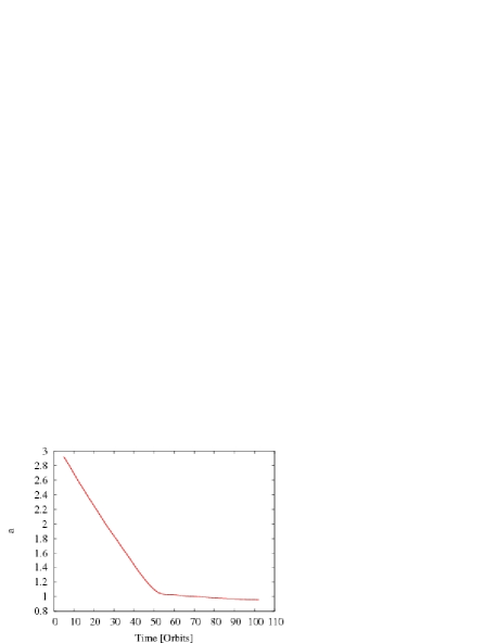
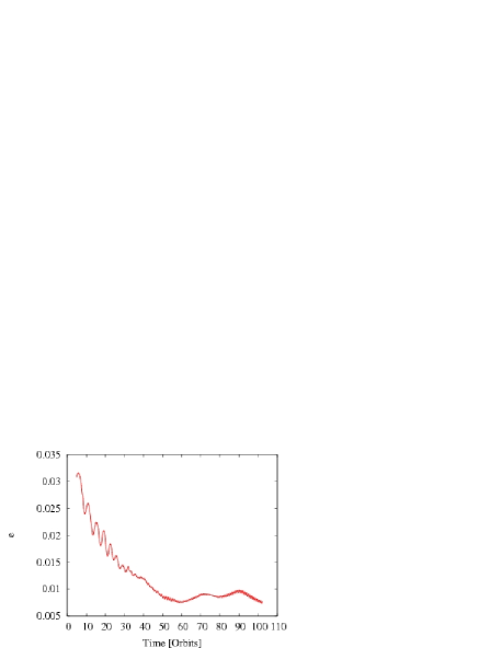
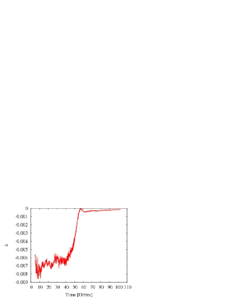
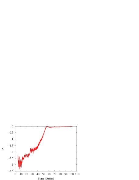
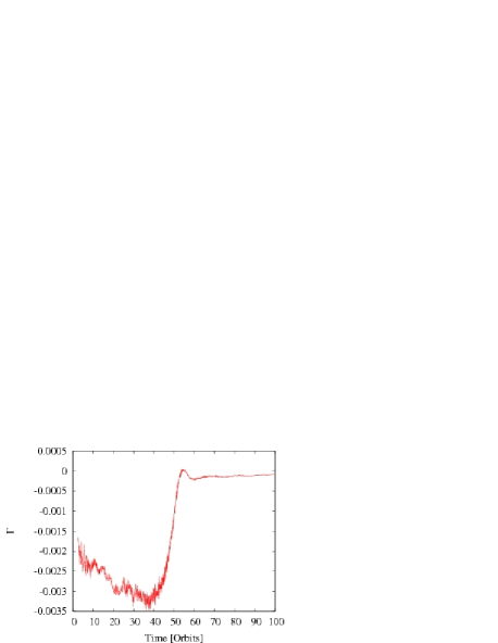
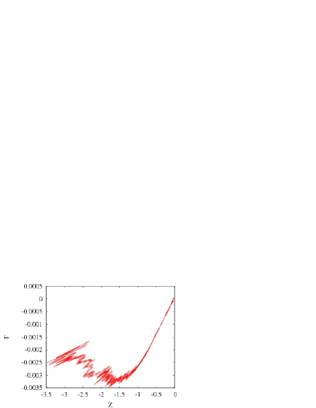
Figure 1: Orbital evolution for the standard case. The upper left and upper right panels show the evolution of the planet’s semi-major axis $a$ and eccentricity $e$. The evolution of the migration rate $\dot{a}$ and the non-dimensional migration rate $Z$ are presented in middle left and middle right panels. The lower row shows the total torque $\Gamma$ exerted by the gas on the planet. Left and right panels present the torque as a function of time and as a function of the non-dimensional migration rate $Z$, respectively.

5.1 Orbital evolution

The planet’s orbital evolution is shown in Fig. 1. Looking at the semi-major axis (upper left panel) we can divide the planet’s orbital evolution into two stages. The first one is the rapid migration stage, which lasts for about $60$ orbits and corresponds to the type III migration regime. During this stage, the planet migrates rapidly due to the co-orbital flow and is not able to clear a full gap. The migration rate $\dot{a}$ (middle left panel) is initially close to constant around $-0.0065$, but after $t=40$ orbits, $|\dot{a}|$ starts to decrease rapidly. This behaviour is caused by the strong mass accumulation in the planet’s proximity (see Sect. 5.3 and Fig. 3). As the migration slows down some of this mass is lost again, giving $\dot{a}$ close to zero near $t=55$ orbits. The dimensionless migration rate $Z$ (middle right panel) shows essentially the same behaviour but since $\dot{a}_{\mathrm{f}}\sim a^{-0.5}({\widetilde{M}}_{\mathrm{P}}/M_{\mathrm{S}})^{2/3}$, it decreases even when $\dot{a}$ is almost constant. The important transition from the fast ($|Z|>1$) to the slow ($|Z|<1$) migration limit takes place at about $47$ orbits.

The migration slows down as $a=1$ is approached. In the second stage (after $60$ orbits) the planet migrates slowly enough to allow a gap to open up. To avoid confusion with the concept of the slow migration limit (defined as $|Z|<1$), we will refer to this second stage as the gap opening stage. The $|\dot{a}|$ decreases slowly and is equal $1.5\times 10^{-4}$ at $t=100$ orbits, giving a migration time-scale $\tau_{\mathrm{M}}=a/\dot{a}$ equal $1.3\times 10^{4}$ yr. Note that this is not classical type II migration, as the total torque is not dominated by the the differential Lindblad torque. However, as the corotation torque $|\Gamma|$ slowly decreases with time, the system may ultimately make the transition to type II migration.

The time evolution of the total torque $\Gamma$ exerted by the gas on the planet is plotted in the lower left panel. In the rapid migration stage the migration is driven by the corotation torque $\Gamma_{\mathrm{CR}}$ and the total torque $\Gamma$ is dominated by $\Gamma_{\mathrm{CR}}$, the differential Lindblad only playing a negligible role. Unlike the migration rate, $|\Gamma|$ grows during the first $40$ orbits, and then rapidly drops due to the strong mass accumulation in the planet’s proximity and the transition from the fast to the slow migration limit. The corotation torque is closely related to the migration rate, as illustrated in the lower right panel. The plot shows $\Gamma$ versus the non-dimensional migration rate $Z$. What is most notable is that the total torque $|\Gamma|$ grows linearly with $|Z|$ for the slow migration limit. In the fast migration limit the relation between $Z$ and $\Gamma$ is non-linear and the torque saturates around $Z\approx-1.5$. $|\Gamma|$ reaches its maximum value at $Z\approx-1.7$. It is consistent with Fig. 9 in Masset & Papaloizou (2003).

In the gap opening stage $\Gamma$ evolves toward zero (it is equal $-1.8\times 10^{-4}$ and $-1.1\times 10^{-4}$ at $75$ and $100$ orbits respectively), but is still larger than the predicted differential Lindblad torque. This is caused by a small mass outflow from the interior of the Roche lobe, which increases $|\Gamma|$. In models where mass accretion on the planet is allowed, this mass outflow is much more limited and the final torque is an order of magnitude smaller.

The upper right panel in Fig. 1 shows the changes of the eccentricity $e$. The eccentricity grows rapidly during the first few orbits and reaches 0.03, after that decreasing with time. In the gap opening stage $e$ becomes $e<0.01$. We postpone further discussion of the eccentricity evolution to Sect. 8.

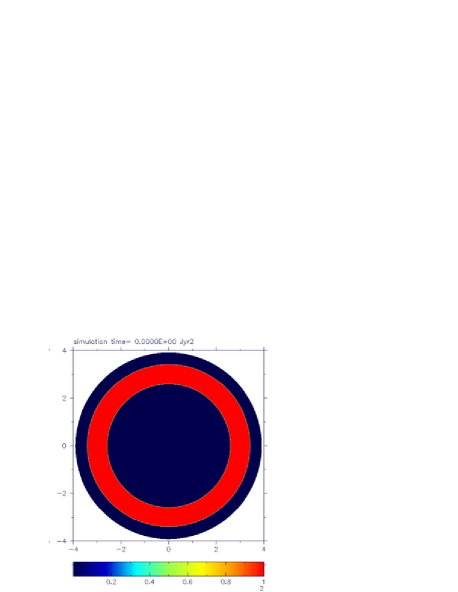
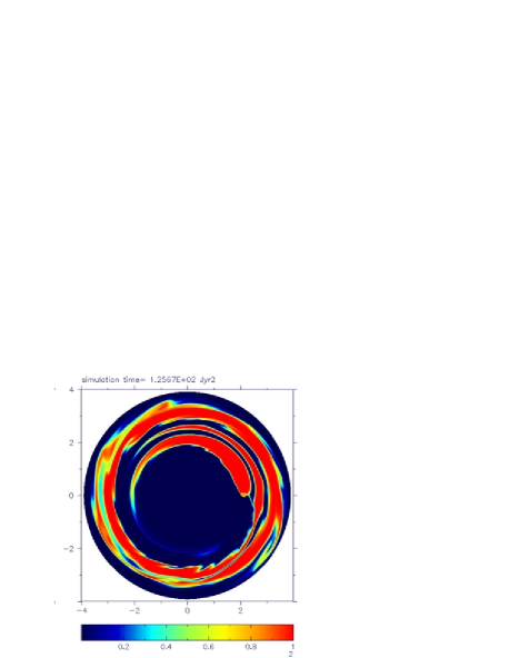
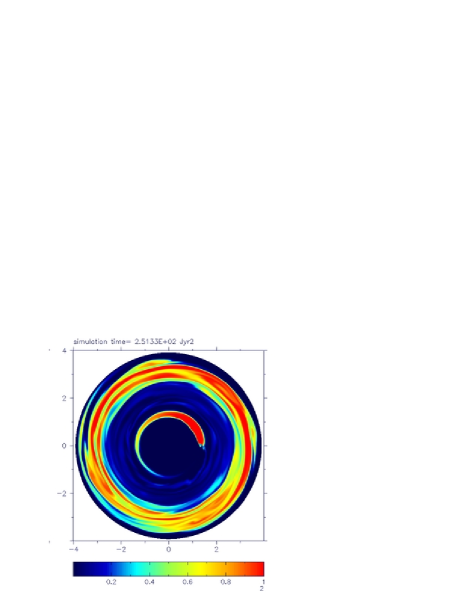
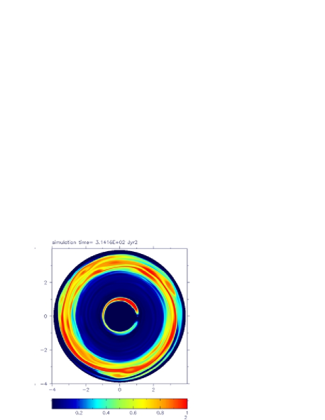
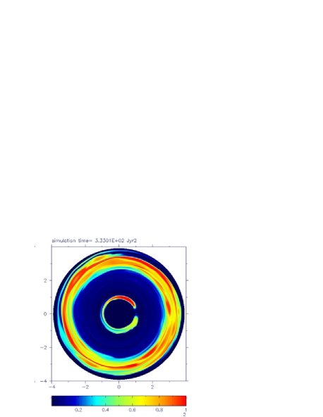
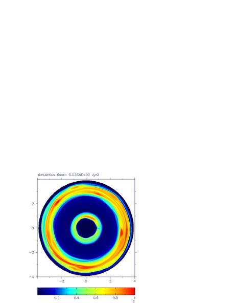
Figure 2: The mass fraction of the gas that initially was placed in the corotational region $a_{\mathrm{init}}-2R_{\mathrm{H}}<r_{\mathrm{s}}<a_{\mathrm{init}}+2R_{\mathrm{H}}$, where $r_{\mathrm{s}}$ is the distance to the star and $a_{\mathrm{init}}$ is the planet’s initial semi-major axis. The mass fraction goes from $0$ (gas from the inner disc only) up to $1$ (gas from corotation only). The top left panel shows the initial condition. The top right ($t=20$ orbits, $Z\approx-2.35$) and a middle left ($t=40$ orbits, $Z\approx-1.4$) present the fast migration limit. The middle right ($t=50$ orbits, $Z\approx-0.4$) and a bottom left ($t=53$ orbits, $Z\approx-0.05$) show the slow migration limit. The last panel displays the mass fraction during the gap opening stage ($t=80$ orbits, $Z\approx-0.046$). All plots are in a co-moving reference frame with the planet at $(x,y)=(3,0)$, $(2.25,0)$, $(1.44,0)$, $(1.1,0)$, $(1.05,0)$ and $(0.99,0)$ respectively.

5.2 Flow structure in the co-orbital region

In this section we discuss the relation between the corotational torque $\Gamma_{\mathrm{CR}}$ and the asymmetry of the horseshoe region. The latter is connected to the the non-dimensional migration rate $Z$, since $Z$ expresses the ratio of the migration to libration time scales. In the slow migration limit ($|Z|<1$) $T_{\mathrm{migr}}$ is longer than $T_{\mathrm{lib}}$ and the horseshoe region can extend the full $2\pi$ in azimuth. For $|Z|>1$ the horseshoe region shrinks into a single tadpole-like region. Once this happens the rest of the co-orbital region is taken up by a flow from the inner to the outer disk. We will denote this flow as well as the region it goes through as the co-orbital flow.

In the simulation $Z$ evolves from $-3$ to $0$ (middle right panel in Fig. 1), and thus the morphology of the co-orbital region should show an evolution from tadpole to a regular horseshoe shape. To study this we use the tracer fluid to follow the gas that was placed in the initial corotational region ($a_{\mathrm{init}}-2R_{\mathrm{H}}<r_{\mathrm{s}}<a_{\mathrm{init}}+2R_{\mathrm{H}}$). Figure 2 shows the evolution of this tracer fluid, with the top left panel displaying the initial condition.

The top right and middle left panels present the mass fraction during the fast migration phase for $Z=-2.35$ ($t=20$ orbits) and $Z=-1.4$ ($t=40$ orbits). Due to the planet’s fast inward migration, most of the gas placed initially in the co-orbital region is left in its initial position and only a small fraction of mass is captured by the planet in the horseshoe region. The gas flow there is strongly asymmetric and the region shrinks to a single tadpole-like region around the L4 libration point. It has relatively sharp edges and the gas captured by planet almost does not mix with the gas crossing the co-orbital region. The azimuthal extent of the horseshoe region grows slowly with decreasing $|Z|$ and is about $\pi$ and $1.2\pi$ for $Z$ equal $-2.35$ and $-1.4$ respectively. This means that the co-orbital flow takes up a wide range in azimuth, that is only weakly dependent on $Z$. Consequently, the mass flux of the gas crossing corotation depends mostly on the initial density profile, and the co-orbital torque $\Gamma_{\mathrm{CR}}$ is a linear function of $M_{\mathrm{\Delta}}$, almost insensitive to the changes of $Z$. We should keep in mind that $M_{\mathrm{\Delta}}$ is not a really an independent variable, since it depends on the way the horseshoe region is populated, which depends on the migration history and thus indirectly on the previous values of $Z$.

The volume of the co-orbital region is given by $V_{\mathrm{CR}}=4\pi ax_{\mathrm{s}}$, and thus decreases for inward migration, as can be seen in Fig. 2. This is important since the mass deficit is a function of $V_{\mathrm{CR}}$ and of the difference in the density flux between the co-orbital flow ($\Sigma_{\mathrm{s}}$) and the horseshoe region that moves together with the planet ($\Sigma_{\mathrm{g}}$, also see Eq. 2). For a constant value of $\Sigma_{\mathrm{s}}-\Sigma_{\mathrm{g}}$, the torque would thus decrease as $V_{\mathrm{CR}}$, i.e.  as $a^{2}$. A slow down of inward migration can thus be caused by this simple geometrical reason. We discuss this and other stopping mechanisms in Sect. 7.

During the entire phase of fast migration, there is a small amount of the gas leaving the horseshoe region. This is visible in Fig. 2 as a light-blue leading spiral.

As $|Z|$ drops, the horseshoe region grows in azimuth and the co-orbital flow region shrinks. For $|Z|\approx 1$ the horseshoe region fills the whole co-orbital region, and the simulation enters the slow migration limit. In the presented simulation the surface density at $5.2$ AU is equal $523$ g cm^-2 and $\Sigma\sim r^{-1}$, and the transition between fast and slow migration limit happens when the planet is at $6.2$ AU. In the slow migration limit phase the flow through the corotation is limited to a narrow stream at the boundary of the Roche lobe and the asymmetry in the horseshoe region is relatively small. However, this small asymmetry is sensitive to small changes in $Z$, giving a strong dependence of $\Gamma_{\mathrm{CR}}$ on $Z$. As the flow becomes more symmetric both globally (shape of the horseshoe orbits) and locally (shape of orbits in the planets vicinity; see Sect. 5.3), $\Gamma$ diminishes rapidly.

The middle right and bottom left panels present the mass fraction for the slow migration limit for $Z=-0.4$ ($t=50$ orbits) and $Z=-0.05$ ($t=53$ orbits). In this phase the planet’s radial motion is slow and a gap is being cleared. Although the azimuthal extent of the horseshoe region is close to $2\pi$ for both values of $Z$, the shape of the horseshoe streamlines differ between the two snapshots. In the earlier case an asymmetry is still visible, but in the later one some gas from the inner disc has been trapped in the tadpole region around the L5 Lagrange point and the asymmetry is starting to disappear. In this phase of migration the second tadpole region is created and the gas from the co-orbital flow mixes with the gas carried along with the planet. On both panels there is a visible flow through the co-orbital region, but in the second case this flow is dominated by gas leaving the planet’s vicinity. This lowers $\Gamma$ and gives $\dot{a}\approx 0$ at about $55$ orbits.

The last panel displays the mass fraction after the planet has almost opened a gap ($t=80$ orbits, $Z=-0.046$). In this case the asymmetry of horseshoe streamlines is almost invisible, and the gas flow through the co-orbital region is very small. We can still see a difference between the tadpole regions around the L4 and L5 Lagrange points. Most of the gas around L4 has been carried along with the planet, but the gas around L5 was mostly captured during the last phase of migration.

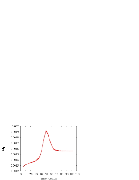
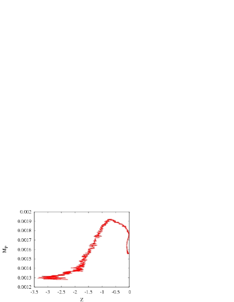
Figure 3: The evolution of the effective planet mass for the standard case. The left and right panels present the effective planet mass as a function of time and of the non-dimensional migration rate, respectively. The initial planet mass is $M_{\mathrm{P}}=0.001$. During the first $40$ orbits the migration rate $\dot{a}$ is almost constant and the rate of the mass accumulation $\dot{\widetilde{M}}_{\mathrm{P}}$ remains constant too. $\dot{\widetilde{M}}_{\mathrm{P}}$ increases when migration slows down. After the planet enters the gap opening stage at about $60$ orbits the planet loses about 14% of its mass and at the end of simulation ${\widetilde{M}}_{\mathrm{P}}=0.00156$.

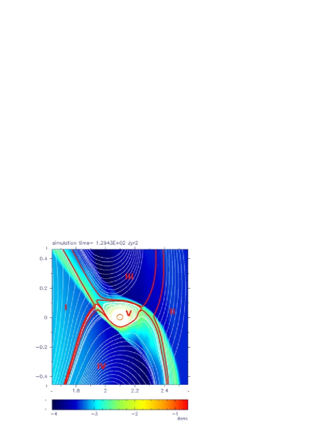
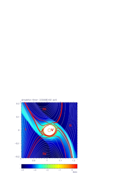
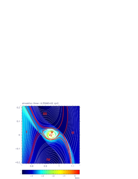
Figure 4: The surface density and flow lines in the planet’s vicinity for the standard case at four different stages of migration. The upper left panel corresponds to the fast migration limit with $Z\approx-2.35$, $t=20$ orbits. The upper right and lower left panels show slower migration ($Z\approx-1.1$, $t=46$ orbits and $Z\approx-0.05$, $t=56$ orbits) with the circumplanetary disc quickly gaining and losing mass respectively. The last panel (lower right) presents the stage of the gap opening planet ($|Z|\ll 1$, $t=100$ orbits) with an almost constant mass of the circumplanetary disc. The colour scale is logarithmic. The plotted domain is square region of the size of $6R_{\mathrm{H}}$. The flow lines close to the border of different regions are made more visible. There are five regions marked in the plots: inner (I) and outer (II) disc, the co-orbital region (III and IV) and the circumplanetary disc (V). On the upper panels the regions III and IV denote the horseshoe and co-orbital flow regions, respectively.

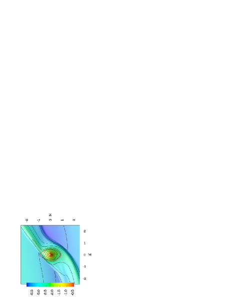
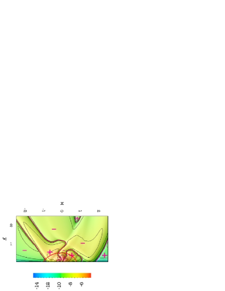
Figure 5: The density distribution and the asymmetry in the torque distribution in the planet’s vicinity for the fast migration limit with the low mass accumulation rate ($Z\approx-2.35$, $t=20$ orbits). The left panel shows the surface density averaged over 5 orbits. The right panel presents the absolute value of the sum $\Gamma_{\mathrm{c}}(x_{\mathrm{p}},y_{\mathrm{p}})+\Gamma_{\mathrm{c}}(x_{\mathrm{p}},-y_{\mathrm{p}})$. The borders of the regions giving positive (+) and negative (-) contributions to the total torque are shown by thick pink lines. The red line shows the Roche lobe size. The plots cover $5R_{\mathrm{H}}$ and the planet is placed at the centre. The colour scale is logarithmic.

5.3 Mass accumulation and flow structure in the planet’s vicinity

In the previous section we described the relation between the non-dimensional migration rate and the asymmetry of the gas flow in the full co-orbital region. We will now focus on the local gas flow near to the planet. Just as we saw for the whole co-orbital region, the planet’s fast radial motion also strongly influences the gas evolution inside its Roche lobe, causing the circumplanetary disc to acquire an asymmetric shape. The co-orbital flow enters the Roche lobe and after interacting with the gas in the planet’s proximity, will partly be captured into the circumplanetary disc. We have found this mass accumulation to be an important ingredient in our simulations of type III migration, determining the flow structure in the planet’s vicinity and the torque generated within the Roche lobe.

In our standard simulation, the effective gravitational planet mass was increased by the mass content within the smoothing length $\widetilde{M}_{\mathrm{P}}=M_{\mathrm{P}}+M_{\mathrm{soft}}$, where the smoothing length corresponds to the “surface” of the planet (Peplinski et al., 2007a). The time evolution of $\widetilde{M}_{\mathrm{P}}$ is presented in the left panel of Fig. 3. During the first $40$ orbits the migration rate is approximately constant, as is the mass accumulation rate. During this time the mass contained within the smoothing length $M_{\mathrm{soft}}$ reaches about 45% of the initial planet mass. The mass of the gas inside the whole Hill sphere amounts to about 55% of the initial mass, so most of this material is found inside the planet’s gravitational smoothing length.

The mass accumulation rate increases sharply when the planet starts to slow down at $t=40$ orbits. In the relatively short time of $10$ orbits $M_{\mathrm{soft}}$ increases up to 90% of the initial planet’s mass and a strong pressure gradient forms around the planet. This pressure gradient is supported by the gas inflow into the circumplanetary disc. The large mass accumulation rate is made possible by our use of a locally isothermal equation of state that makes the circumplanetary disc aspect ratio independent of the gas density. For the same reason the accumulated mass leaves the Hill sphere shortly after the rapid migration has stopped. This affects the total torque $\Gamma$ giving the positive value of $\dot{a}$ during this short period (Fig. 1, middle panels).

When the simulation reaches the second, gap opening stage, $M_{\mathrm{soft}}$ remains approximately constant at 56% of $M_{\mathrm{P}}$.

The relation between the planet’s effective mass ${\widetilde{M}}_{\mathrm{P}}$ and $Z$ is presented in right panel of Fig. 3. $\dot{\widetilde{M}}_{\mathrm{P}}$ is low and almost constant during the fast migration limit phase and rapidly grows when $Z$ reaches $-1.7$, causing the total torque to decrease (lower right panel in Fig. 1). The next important change takes place in the slow migration limit phase at $Z\approx-0.6$, when the planet starts to open a gap and $\widetilde{M}_{\mathrm{P}}$ starts to decrease. We note that the evolution of $\widetilde{M}_{\mathrm{P}}$ is strongly dependent on choice for the circumplanetary disc aspect ratio $h_{\mathrm{p}}$, but for the given value of $h_{\mathrm{p}}=0.4$ the evolution of $M_{\mathrm{P}}$ is almost independent of the other parameters, such as $r_{\mathrm{soft}}$. For more discussion on this, see Sect. 6 and Paper I.

Since the mass accumulation rate determines the structure inside the Roche lobe, we now discuss the flow in the planet’s vicinity for four different stages of the simulation: the rapid migration stage with and without the fast mass accumulation in the circumplanetary disc, the stage of mass outflow from the planet’s proximity and the final gap opening stage with an approximately constant effective planet mass. They are presented in Fig. 4. The plots show the surface density and the flow lines. The flow lines close to the border of different regions have been made more visible. There are five regions marked in the plots: inner (I) and outer (II) disc, the co-orbital region (III and IV) and the circumplanetary disc (V). It should be realized that the gas evolution inside the Roche lobe is variable and we present just a few snapshots to describe important differences between different stages of simulation.

The upper left panel of Fig. 4 corresponds to the fast migration limit with $Z\approx-2.35$ and a relatively low mass accumulation rate $\dot{\widetilde{M}}_{\mathrm{P}}$. In this case region III is the horseshoe region and IV the co-orbital flow. The orbits in the circumplanetary disc are found to be strongly asymmetric, compressed at the side of the co-orbital flow and stretched at the side of the horseshoe region. The asymmetry of the bow shocks and the flow lines in the co-orbital region is also visible. The whole horseshoe region is shifted backwards with respect to the planet’s radial motion, and the left bow shock is compressed into a straight line, whereas the right bow shock is stretched and more curved. In this phase the mass accumulation is still rather modest; closer investigation shows the circumplanetary disc to be fed by both regions III and IV. The averaged density and the torque asymmetry distribution for this stage of migration are presented in Fig. 5.

The stage of strong mass accumulation near the transition from the fast to the slow migration limit ($Z\approx-1.1$) is presented in upper right panel in Fig. 4. The asymmetry of the bow shocks and the flow lines in the co-orbital region is still visible, however the orbits in the circumplanetary disc have become less regular. The interior of the Roche lobe is strongly disturbed by the gas inflow from the inner disc I and the horseshoe region III and the flow lines are very time variable. In spite of this, the circumplanetary disc no longer shows the asymmetry seen in the previous phase, which explains the lower value for the torque $\Gamma$.

The asymmetry of the bow shocks and the circumplanetary disc disappears in the next stage. The lower left panel shows the flow lines near the planet during the slow migration limit phase ($Z\approx-0.05$) and strong mass outflow. As we saw in the previous section, in this stage the horseshoe region extends over the whole azimuthal range and the planet starts to open a gap. The whole co-orbital region also becomes more symmetric and regular. The gas leaves the circumplanetary disc flowing along the bow shocks and influences the flow lines at the border of the Roche lobe, but the orbits inside the circumplanetary disc are regular.

The last panel (lower right) presents the stage of the gap opening planet $|Z|\ll 1$, with an almost constant mass in the circumplanetary disc. In this stage the gap is almost cleared and the co-orbital region is symmetric. Although the mass inside the Hill sphere is almost constant some outflow from the Roche lobe can still be seen. The most important difference with the previous stages is the shape of the flow lines in the planet’s vicinity. In the previous stages the gas was orbiting the planet creating a circumplanetary disc, however in this last stage the large pressure gradient prevents circular orbits in the planet’s proximity. We have to note that this stage looks different for models with an accreting planet (see Paper I, Sect. 5.1.2). In that case the planet is surrounded by the Keplerian-like sub-disk and there is no gas outflow from the Roche lobe during the last phase of migration. This is consistent with what was found by D’Angelo et al. (2003).

After having described the flow structure we now consider the torque distribution in the planet’s vicinity. We focus on the first stage, i.e. rapid migration with a low mass accumulation rate ($t=20$ orbits). This corresponds to the upper left panel of Fig. 4. In the left panel of Fig. 5 we present the surface density averaged over 5 orbits for $Z\approx-2$. The plot covers $5R_{\mathrm{H}}$ and the planet is placed at the centre. The red line shows the Roche lobe size. The asymmetry between the left and right bow shock which we described above, is clearly visible. Although the left bow shock is sharper and has a higher density close to the planet, the overall amount of mass at the right bow shock is higher, since the density increase close to the right bow shock extends over a much wider area. The plot also shows the averaged surface density to be lower in the horseshoe region (positive values of $y$) than in the co-orbital flow (negative values of $y$). This asymmetry causes the right bow shock to have a larger contribution to the total torque $\Gamma$ than the left one. This is further illustrated in the right panel of Fig. 5, where we show the absolute value of the sum $\Gamma_{\mathrm{c}}(x_{\mathrm{p}},y_{\mathrm{p}})+\Gamma_{\mathrm{c}}(x_{\mathrm{p}},-y_{\mathrm{p}})$, where $\Gamma_{\mathrm{c}}$ is the torque generated by a single grid cell and $(x_{\mathrm{p}},y_{\mathrm{p}})$ is the position of the cell with respect to the planet. The borders of the regions giving positive (+) and negative (-) contributions to the total torque are shown with pink lines. The left and the right bow shocks give positive and negative contributions, respectively. Although the absolute value of the torque sum is similar for both shocks, the right bow shock is much wider and its contribution to $\Gamma$ dominates. The region between the two shocks gives a negative contribution showing that the torque generated by the co-orbital flow is stronger than the torque generated by the horseshoe region.

The interior of the Roche lobe shows three extremes. The two outer ones give a positive contribution and the middle one a negative. These extrema are the result of the asymmetry of the circumplanetary disc, which as we saw above, is compressed at the side of the co-orbital flow and stretched at the side of the horseshoe region. However the sum of these extremes nearly cancels, and the overall torque generated within the Roche lobe is found to be negative. This once more illustrates the point made in Paper I, that the interior of the Roche lobe cannot be treated as a system isolated from the co-orbital flow and that the torques from this inner region have to be taken into account when studying type III migration (for more discussion, see Peplinski et al. (2007a)).

We would like to repeat here that we only show one snapshot here, but that the gas flow in the planet’s vicinity is highly variable, with changes in the shapes of bow shocks and the circumplanetary disc, causing the large variations in $\Gamma$ seen in the lower panels of Fig. 1

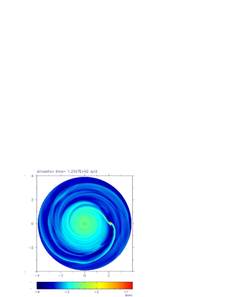
Figure 6: Global surface density for the standard case at $t=20$ orbits. The planet has migrated from $a=3$ to $a=2$. The colour scale is logarithmic. The planet’s location is $(x,y)=(2.3,0)$

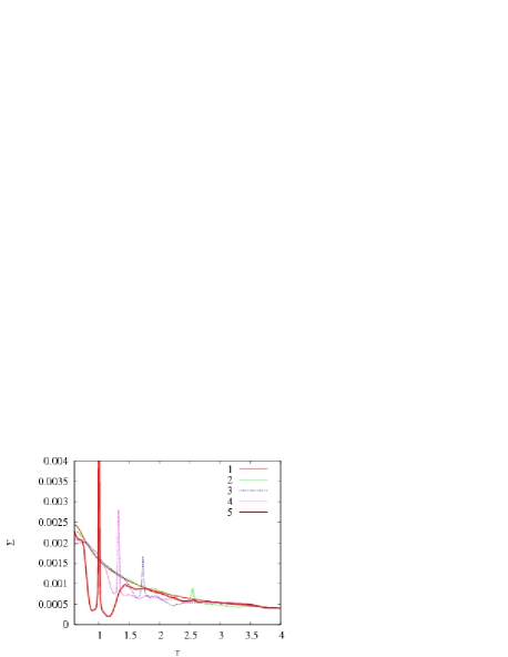
Figure 7: The azimuthal average of the surface density $\Sigma$ for times $t=0$, $10$, $30$, $50$ and $60$ orbits (curves 1, 2, 3, 4 and 5 respectively). During the rapid migration phase no gap is formed (curves 1 to 4). The last curve corresponds to the gap opening stage The planet position is visible as a spike in the density profile.

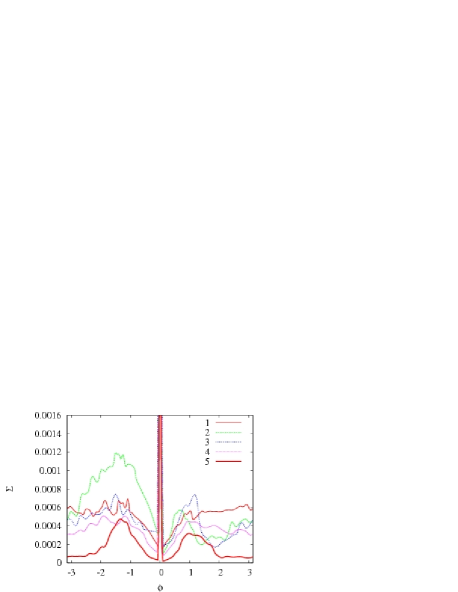
Figure 8: The surface density $\Sigma$ along an azimuthal cut through the planet position for times $t=10$, $30$, $50$, $60$ and $100$ orbits (curves 1, 2, 3, 4 and 5 respectively). The negative and positive values of $\phi$ correspond to the co-orbital flow and horseshoe region, respectively. The planet is located at $\phi=0$.

5.4 Surface density

To gain further inside into the migration process, we now study the surface density distribution in the disc. A colour scale plot of the global surface density distribution for the fast migration limit phase at $t=20$ orbits ($Z\approx-2.35$) is displayed in Fig. 6. In this phase the planet does not yet open a gap due to its fast radial motion. For the same reason the surface density in the inner disc does not show significant differences from the initial condition. There are two lower density regions at the planetary radius corresponding to the horseshoe region (positive $y$) and the co-orbital flow region (negative $y$). The detailed structure of the surface density distribution in the planet vicinity is shown in Fig. 5.

To study the time evolution of the surface density $\Sigma$ we use a series of plots showing this quantity in the radial and azimuthal direction. Fig. 7 presents the azimuthal average of $\Sigma$ over $2\pi$ at times $t=0$, $10$, $30$, $50$ and $60$ orbits (curves 1, 2, 3, 4 and 5 respectively). The average surface density is weakly modified outside the planet’s co-orbital region. During the rapid migration phase (curves 1, 2, 3 and 4) no gap is cleared, but the planet is followed by a lower density region. The main reason for this depletion in $\Sigma$ in the planet’s neighbourhood is the mass accumulation in the planet vicinity and the fact, that after an interaction with the planet the gas crossing the co-orbital region is spread over a region with a radial size of a few $x_{\mathrm{s}}$. The last curve in Fig. 7 corresponds to the gap opening stage ($\dot{a}$ approaching the value for type II migration).

Fig. 8 shows $\Sigma$ along an azimuthal cut through the planet position for time $t=10$, $30$, $50$, $60$ and $100$ orbits (curves 1, 2, 3, 4 and 5 respectively). It illustrates the difference between the density of the horseshoe region ($\Sigma_{\mathrm{g}}$) and the co-orbital flow region ($\Sigma_{\mathrm{s}}$), that drives type III migration. The region of co-orbital flow and the horseshoe region are found at the negative and positive values of $\phi$, respectively. The fast migration limit phase is represented by curves 1 and 2. Initially the asymmetry in $\Sigma$ is only located inside the Roche sphere (only barely visible on the plot due to adopted scale), but in time it grows in azimuth showing a large difference in $\Sigma$ between the L4 and L5 Lagrange points. During the fast migration limit phase the L5 point is moved in the direction of the planet (compare the position of the density maximum for positive $\phi$ in curves 2 and 5). The asymmetry decreases in the slow migration limit phase (curve 3) and becomes unimportant when a gap starts opening up (curves 4 and 5). During the whole simulation the surface density has maxima at the L4 and L5 points and decreases in the direction of the planet.

To further illustrate the asymmetry, Fig. 9 shows radial surface density cuts through L5 (curve 3) and L4 (curve 4), together with the azimuthal average of the surface density (curve 2). Curve 1 shows the initial density profile. The upper left and right panels show these quantities during the fast migration limit phase ($t=30$ and $40$ orbits, respectively) and the lower left and right panels the same during the slow migration limit phase ($t=50$ and $60$ orbits). The cut through L4 gives the approximate width of the co-orbital region and the density $\Sigma_{\mathrm{g}}$ inside the horseshoe region. Similarly the cut through L5 gives the approximate value of the density of the gas crossing the co-orbital region $\Sigma_{\mathrm{s}}$. The difference between $\Sigma_{\mathrm{s}}$ and $\Sigma_{\mathrm{g}}$ is the main reason for the rapid migration.

In the fast migration limit the planet carries along the low density horseshoe region which has well defined, sharp edges and a width $x_{\mathrm{w}}\approx 2R_{\mathrm{H}}$. $\Sigma_{\mathrm{g}}$ is lower than the initial density at the initial planet position $r=3$ and almost does not change in time. In contrast, $\Sigma_{\mathrm{s}}$ is close to the initial density profile at the current planet’s position. $\Sigma_{\mathrm{g}}$ and $\Sigma_{\mathrm{s}}$ differ from each other in the whole co-orbital region. The cut through L5 shows also the low density region following the planet. It is caused by the spreading of the gas over a few $x_{\mathrm{w}}$ and compression at the two shocks in the outer disc region (see Fig. 6).

In the slow migration limit (lower left panel) the density around L5 drops significantly, as the horseshoe region gets more extended and the co-orbital region becomes more symmetric. At the same time the density inside the horseshoe region increases slowly. The asymmetry between the density cuts through L4 and L5 is now only visible at the inner edge of the co-orbital region. In the last, gap opening stage of migration $Z\ll 1$ (lower right panel) the co-orbital region becomes symmetric and the density cuts through L4 and L5 are similar. The planet starts to opens a gap and the density in the horseshoe region decreases.

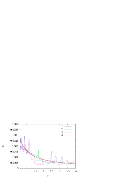
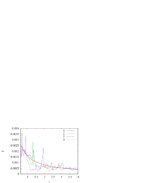
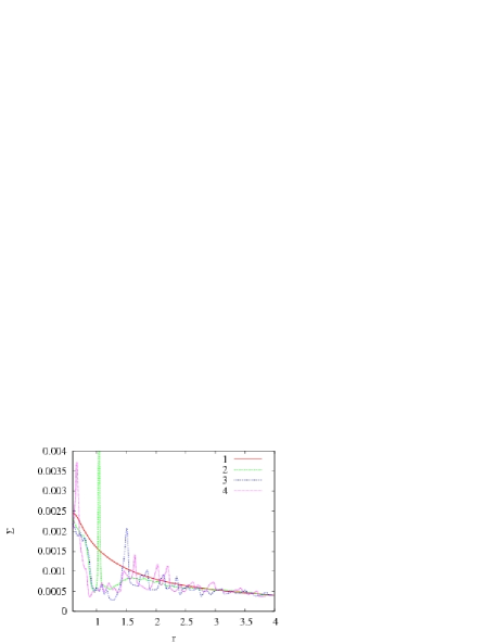
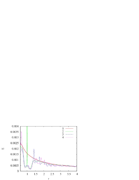
Figure 9: The evolution of the density profiles in the standard case. Each panel shows the initial density profile (curve 1), the azimuthal average of the surface density (curve 2; the planet position is visible as a spike) and the surface density cuts through the Lagrange points L5 (curve 3) an L4 (curve 4). The panels upper left, upper right, lower left and lower right show the density profiles after $30$, $40$, $50$ and $60$ orbits, respectively.

6 Dependence on the simulation parameters

After having described type III migration in detail for one standard case, we now consider the dependence of the planet’s orbital evolution on the most important simulation parameters.

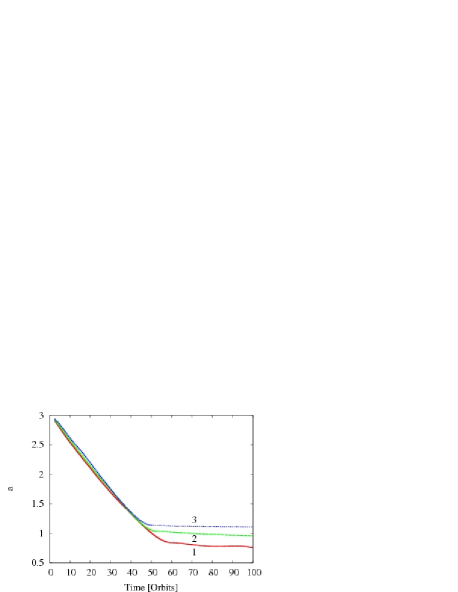
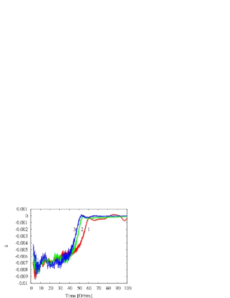
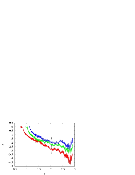
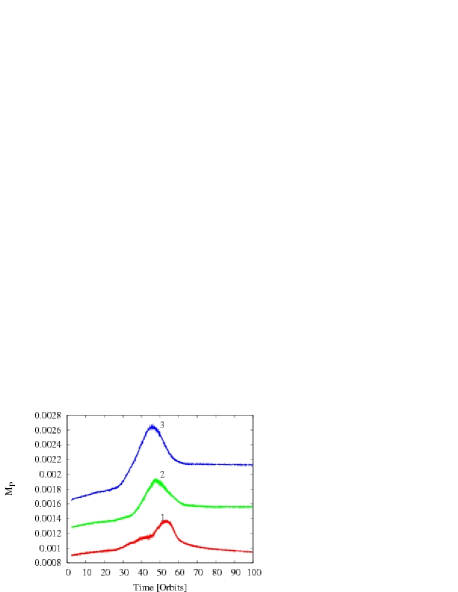
Figure 10: Results of the simulations for different planet masses. Curves 1, 2 and 3 correspond to the initial planet mass $M_{\mathrm{P}}$ equal $0.0007$, $0.001$ (standard case) and $0.0013$, respectively. The upper left and upper right panels show the evolution of the planet’s semi-major axis $a$ and the migration rate $\dot{a}$. The non-dimensional migration rate $Z$ as a function of the planet’s position in the disc and the evolution of the effective planet mass $\widetilde{M}_{\mathrm{P}}$ are presented in the lower left and lower right panels. During the first $40$ orbits (fast migration limit $|Z|>1$) all systems evolve almost exactly the same way even though the (effective) planet mass may vary. The simulations start to differ after reaching the slow migration limit. Even though the migration rate $\dot{a}$ is almost identical for all simulations during the fast migration limit, the non-dimensional migration rates $Z$ differ slightly, since $\dot{a}_{\mathrm{f}}$ depends on $\widetilde{M}_{\mathrm{P}}$.

6.1 Planet’s mass

The first parameter we consider is the planet’s mass. In our investigation we concentrate on the orbital evolution of giant planets. The results of the simulations with the initial mass $M_{\mathrm{P}}$ equal $0.0007$ and $0.0013$ (curves 1 and 3 respectively) are presented in Fig. 10, together with our standard case of $M_{\mathrm{P}}=0.001$

The upper left and upper right panels show the evolution of the planet’s semi-major axis $a$ and migration rate $\dot{a}$. During the first $40$ orbits all systems evolve almost exactly the same way, even though the effective planet masses (lower right panel) differ significantly. This period corresponds to the fast migration limit $|Z|>1$ for all three models. In this phase the orbital evolution is independent of the planet mass since $Z\sim M_{\mathrm{\Delta}}$, and both the non-dimensional migration rate $Z$ and the mass deficit $M_{\mathrm{\Delta}}$ are proportional to $\widetilde{M}_{\mathrm{P}}^{-2/3}$.

Once the planets enter the slow migration limit, the relation between $Z$ and $M_{\mathrm{\Delta}}$ becomes more complicated and their evolution starts to differ. In this phase, $|\dot{a}|$ decreases rapidly and the planet is gradually settles into a type II like migration. Since $Z$ diminishes faster for more massive planets, this transition to the slow migration limit happens sooner for more massive planets, and as a result more massive planets stop their type III migration at larger orbital radii. The final planet’s semi-major axes are $0.75$, $0.95$ and $1.11$ for the initial mass $M_{\mathrm{P}}$ equal $0.0007$, $0.001$ and $0.0013$, respectively.

The relation between the planet mass and its orbital evolution is further illustrated in the lower left panel, where the non-dimensional migration rate $Z$ is plotted as a function of the planet’s position in the disc. A larger planet mass corresponds to a smaller $|Z|$ and thus displaces the orbital evolution curve to the right.

The lower right panel shows the effective mass evolution. For a constant circumplanetary disc aspect ratio $h_{\mathrm{p}}$, higher mass planets accumulate a larger amount of gas in the circumplanetary disc. The mass accumulation rate is relatively low during the fast migration limit and increases with decreasing $|Z|$. There is a visible increase of $\dot{\widetilde{M}}_{\mathrm{P}}$ for $Z\approx-1.7$ in all three cases. Similarly the mass outflow from the Roche lobe starts at $Z\approx-0.6$ independently of the planet mass (and thus happens earlier for more massive planets). The final planet masses are $0.00095$, $0.00155$, $0.0023$ for $M_{\mathrm{P}}$ equal $0.0007$, $0.001$ and $0.0013$ respectively. This corresponds to a relative increase of $35\%$, $55\%$ and $76\%$ after $100$ orbits respectively, and thus the relation between $M_{\mathrm{P}}$ and $\widetilde{M}_{\mathrm{P}}$ is not linear.

The lowest mass planet shows some evolutionary features not seen in the other two. First, its mass accumulation rate shows two instances of rapid growth, the first one at about $27$ orbits ($Z\approx-2.5$), and the second one at $45$ orbits ($Z\approx-1.7$). Second, after $80$ orbits the lowest mass planet shows oscillations in its migration rate. After $120$ orbits these oscillations have damped out, and the migration rate $\dot{a}$ becomes similar to that of the more massive planets. These oscillations are caused by a change of shape of the flow lines in the planet’s vicinity from regular orbits in the circumplanetary disc to a non regular flow modified by the strong pressure gradient.

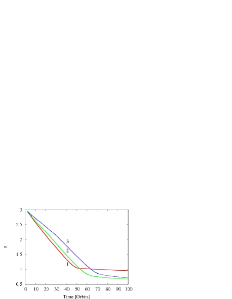
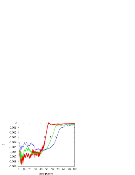
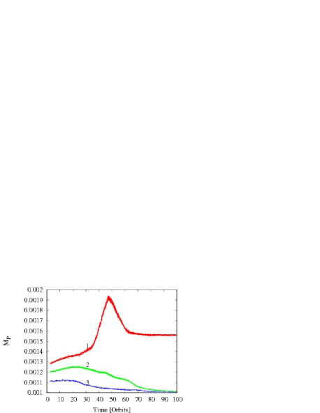
Figure 11: Results of the simulations for the different circumplanetary disc aspect ratios $h_{\mathrm{p}}$. Curves 1, 2 and 3 correspond to $h_{\mathrm{p}}$ equal $0.4$, $0.5$ and $0.6$ respectively. The panels are the same as in Fig. 10.

6.2 Effects of circumplanetary disc aspect ratio

The next parameter we consider is the circumplanetary disc aspect ratio $h_{\mathrm{p}}$. As shown in Paper I, this parameter corresponds to the temperature of the circumplanetary disc, and determines how much material can be accumulated there. Since the mass accumulation influences type III migration, it is interesting to study the effect of this parameter.

In addition to our standard case of $h_{\mathrm{p}}=0.4$, we ran simulations using values of $0.5$ and $0.6$. We do not use a value lower than 0.4, since the tests presented in Paper I showed that a model with 0.3 does not fully converge for the resolution used in our simulations.

The results for all three cases (labelled 1, 2 and 3) are presented in Fig. 11. We use the same set of plots as in Fig. 10: the evolution of the planet’s semi-major axis $a$ and the migration rate $\dot{a}$ in the upper panels, and the non-dimensional migration rate $Z$ as a function of the planet’s position in the disc together with the evolution of the effective planet mass in the lower panels.

As expected, changing $h_{\mathrm{p}}$ has a strong effect on the evolution of the effective planet mass $\widetilde{M}_{\mathrm{P}}$. As we saw above, the standard case (0.4, curve 1) shows a phase of strong mass accumulation, followed by mass loss from the circumplanetary environment after migration has slowed down. The other two cases do not show such strong mass accumulation, and the higher $h_{\mathrm{p}}$, the less mass is accumulated. In fact curves 2 and 3 show that mass outflow already starts at $t\approx 20$ orbits, i.e. during the rapid migration stage.

Considering the evolution of $a$ and $\dot{a}$ we notice some small differences. For $h_{\mathrm{p}}=0.5$ and 0.6 the flow asymmetries in the planet’s vicinity during the fast migration limit phase become less pronounced, leading to a lower total torque $|\Gamma|$. This results in a somewhat lower value for the migration rate $\dot{a}$ during this phase. The start of mass outflow at $t\approx 20$ orbits in these two models leads to a small increase of the migration rate. Consistent with the results from the previous section, the lower final values of $\widetilde{M}_{\mathrm{P}}$ cause the two thicker disc cases to migrate closer to the star. Their type III migration stops at $a\approx 0.7$. It is noticeable that the evolution of the system in the slow migration limit is almost independent of the circumplanetary disc aspect ratio for $h_{\mathrm{p}}\geq 0.5$.

Tracing the evolution in the $Z-r$ plane (lower left panel), all three simulations show similar behaviour until $Z\approx-2$ is reached (lower left panel). After $|Z|$ drops below $1.7$ the model with $h_{\mathrm{p}}=0.4$ starts rapid mass accumulation in the circumplanetary disc, causing it to evolve differently from the other two models.

We have to keep in mind that the assumption of a constant circumplanetary disc aspect ratio is a rather crude one, and in reality this parameter will react to the mass accretion into this disc. More realistic calculations would either need to treat the thermal evolution of the circumplanetary disc self-consistently, or use some approximate recipe relating $h_{\mathrm{p}}$ to $Z$ and the mass accumulation rate. However, the results in this section show that large changes in $h_{\mathrm{p}}$ only have a limited effect on the migration behaviour of the planet.

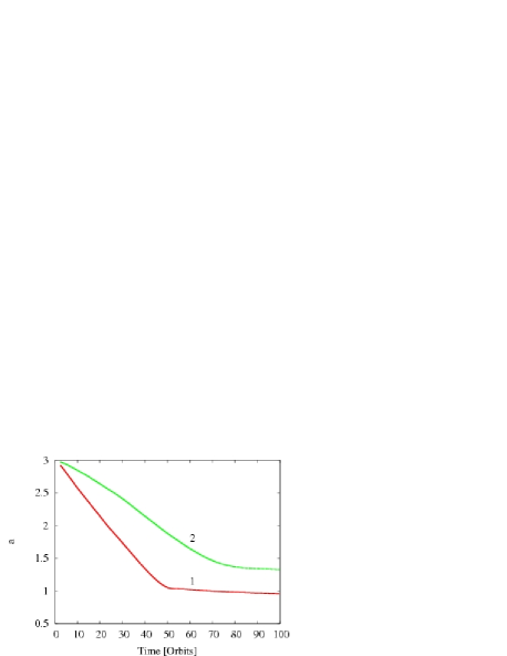
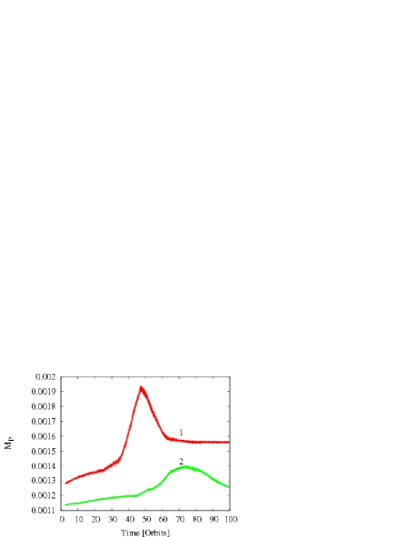
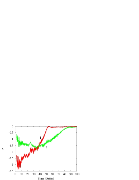
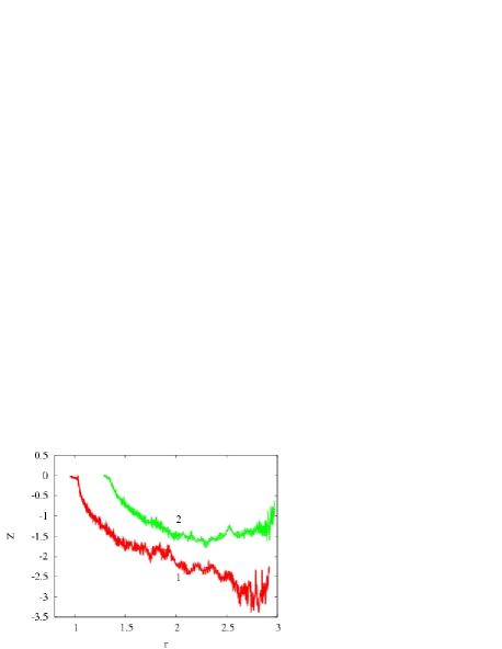
Figure 12: Results of the simulations for different total disc masses. Curves 1 and 2 correspond to the disc to the primary mass ratio $\mu_{\mathrm{D}}$ equal $0.005$ (standard case) and $0.0025$ respectively. The upper left and right panels show the evolution of the semi-major axis and the effective mass; the non-dimensional migration rate $Z$ as a function of time and of radius are presented in the lower left and lower right panels.

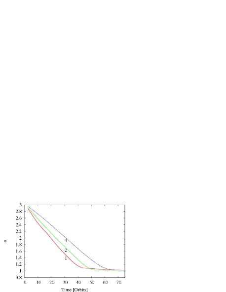
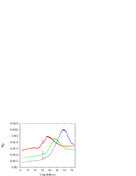
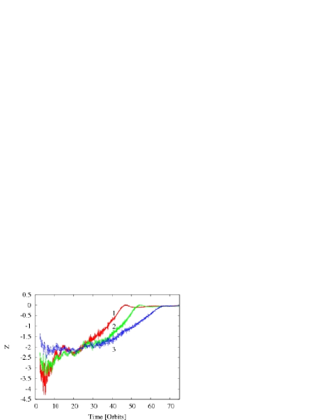
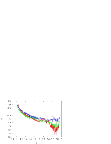
Figure 13: Results of the simulations for the different initial disc profiles with $M_{\mathrm{P}}^{*}=\widetilde{M}_{\mathrm{P}}$. Curves 1, 2 and 3 correspond to $\alpha_{\mathrm{\Sigma}}$ equal $-0.5$, $-1$ (standard case) and $-1.5$ respectively. The layout of the panels is the same as in Fig. 12.

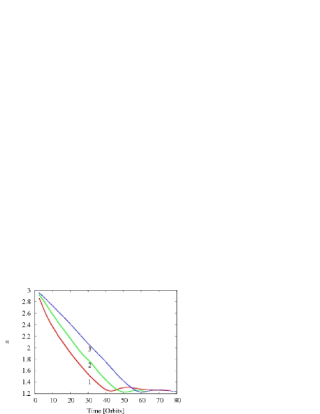
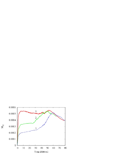
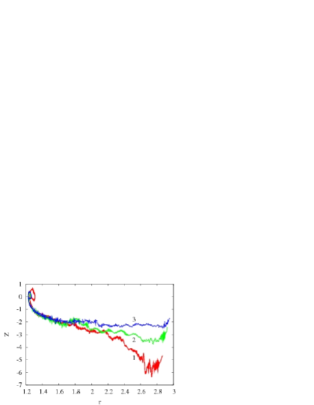
Figure 14: Results of the simulations for the different initial disc profiles with constant $M_{\mathrm{P}}^{*}=M_{\mathrm{P}}=0.001$. Curves 1, 2 and 3 correspond to $\alpha_{\mathrm{\Sigma}}$ equal $-0.5$, $-1$ and $-1.5$ respectively. The layout of the panels is the same as in Fig. 12, except that here the upper right panel shows the evolution of the mass inside the Hill sphere.

6.3 Total disc mass

In the previous two sections we discussed parameters connected to the planet and its circumplanetary disc. In this section and the next we consider parameters defining the circumstellar disc, namely the total disc mass (given by the disc to the primary mass ratio $\mu_{\mathrm{D}}$) and the slope of the initial density profile (described by the exponent $\alpha_{\mathrm{\Sigma}}$), see Sect. 3.3.1.

To study the relation between the total disc mass and the planet migration we compare a simulation with $\mu_{\mathrm{D}}=0.0025$ to our standard case of $0.005$. The other parameters are identical between these two simulations. The results are presented in Fig. 12.

As can be expected the planet migrates slower and less far in the lower mass disc. The stage of the rapid migration lasts longer ($85$ orbits instead of $50$) and the transition between the fast and slow migration limits happens at $60$ orbits, instead of $40$. After the rapid migration ends the planet is locked in the disc at $a=1.3$ ($a=0.95$ for the standard case).

There is no simple relation between the total disc mass and the position where the planet is locked into the disc, or the duration of the rapid migration stage. This is because the migration rate in type III migration depends both on the co-orbital mass deficit $M_{\mathrm{\Delta}}$ and on the asymmetry in the co-orbital region. Changing the total disc mass changes the mass inside the co-orbital region, but the asymmetry depends on the current and previous values of the migration rate. However, $\mu_{\mathrm{D}}$ is an important parameter, since the amount of the mass in the co-orbital region defines the region where rapid migration can take place. Since the volume of the co-orbital region is proportional to $a^{2}$, for the standard smooth density profile with $\alpha_{\mathrm{\Sigma}}\geq-1.5$ it is easier to start rapid migration at larger orbital radii (see the discussion in Masset & Papaloizou 2003). The radii $r=0.95$ and $r=1.3$ are the outer borders of the region, where rapid migration for a Jupiter-mass planet cannot be started for $\mu_{\mathrm{D}}$ equal $0.005$ and $0.0025$ respectively.

The initial value of the migration rate is given by the amount of the gas in the co-orbital region. After about $10$ orbits the non-dimensional migration rates are $Z\approx-2.7$ and $Z\approx-1.4$ (lower left panel in Fig. 12), their ratio indeed matching the ratio of the disk masses. Later both systems evolve differently. The non-dimensional migration rate decreases quickly during the whole stage of rapid migration for the more massive disc, but for the lower mass disc $|Z|$ increases during the first $35$ orbits and then decreases much slower. More similarities between both simulations are visible after plotting $Z$ as a function of the planet’s position in the disc (lower right panel in Fig. 12). Neglecting the first $25$ orbits (region outside $r\approx 1.9$ and $r\approx 2.5$ for the high and low mass disc respectively) the shape of both curves is similar, but the curve for the more massive disc is shifted inward by $0.3$ in radius. This number corresponds exactly to the shift of the boundary of the region where rapid migration is allowed. Decreasing the disc mass thus has a similar effect as increasing the planet mass (lower right panel in Fig. 10).

The effective planet mass (upper right panel in Fig. 12) depends on the total mass of the disc and on the non-dimensional migration rate. It grows slowly in the fast migration limit phase until $|Z|$ drops below $1.7$ after which the mass accumulation rate increases rapidly for both models. The maximum value of the planet mass for both models is reached at $Z\approx-0.6$ at which point the mass outflow from the circumplanetary disc starts. The values are $1.56M_{\mathrm{P}}$ and $1.22M_{\mathrm{P}}$.

6.4 Initial density profile

The next parameter is the exponent $\alpha_{\mathrm{\Sigma}}$. The standard case has $\alpha_{\mathrm{\Sigma}}=-1$ (curve 2 in Fig. 13), and we performed two additional simulations using $-0.5$ and $-1.5$ (curves 1 and 3). All other parameters were taken identical to the standard case. Because of our definition of the surface density, the disc densities are equal at $r=1$, but differ at the initial planet position $r=3$. The $\alpha_{\mathrm{\Sigma}}=-0.5$ case has the largest initial mass in the co-orbital region, and therefore evolves the fastest. It reaches $a\approx 1$ after about $43$ orbits. For the $\alpha_{\mathrm{\Sigma}}=-1.0$ and $-1.5$ cases the planet settles at the same position after about $51$ and $64$ orbits respectively. Because this position is near $r=1$, all three models agree on the final orbital radius, since this is where the surface density is identical between the models, and at a value that is too low to support further rapid migration.

The exponent $\alpha_{\mathrm{\Sigma}}$ determines the average rate with which the non-dimensional migration rate is decreasing and influences the relation between $Z$ and the planet’s position in the disc, which can be seen in the lower right panel. The evolution of the systems differs during the first $16$ orbits only. Later on the relation between $Z$ and $a$ becomes independent of $\alpha_{\mathrm{\Sigma}}$. However, as we will see below this is mostly caused by the evolution of the effective planet mass which is presented in the upper right panel. In the fast migration limit $\widetilde{M}_{\mathrm{P}}$ depends on the initial mass of the co-orbital region (largest for $\alpha_{\mathrm{\Sigma}}=-0.5$) and grows slowly. The mass accumulation rate $\dot{\widetilde{M}_{\mathrm{P}}}$ increases when the planet makes the transition to the slow migration limit. The increase is steep for $\alpha_{\mathrm{\Sigma}}=-0.5$ and relatively smooth for $\alpha_{\mathrm{\Sigma}}=-1.5$. What is important is that $\dot{\widetilde{M}_{\mathrm{P}}}$ has similar values in all presented models and the highest value of $\widetilde{M}_{\mathrm{P}}$ is reached in the simulation with steepest density profile, since the mass accumulation phase takes the longest time there. The final mass of the planet is equal $1.62M_{\mathrm{P}}$, $1.56M_{\mathrm{P}}$ and $1.72M_{\mathrm{P}}$ for $\alpha_{\mathrm{\Sigma}}$ equal $-0.5$, $-1.0$ and $-1.5$ respectively.

To test how the mass accumulation near the planet influences the results we ran a set of simulations where the correction for self-gravity is turned off by keeping the planet mass constant at $M_{\mathrm{P}}^{*}=M_{\mathrm{P}}=0.001$. In these simulations we also introduced an inner disc edge (see Paper I Fig. 2). This edge is not significant for the subject discussed in this section, but it is relevant for the discussion on stopping mechanisms given in the next section. The inner gap starts at $r=1.3$ and the density is constant at $\Sigma=0.00016$ inside $r=0.85$.

The results of these simulations are shown in Fig. 14. The upper left panel shows the planet’s orbital evolution. In all simulations the planet stops its rapid migration at the disc edge. Similarly the transition between the fast and the slow migration limit takes place at the same position, $a=1.28$ close to the initial density maximum. The interaction with the disc edge also leads to a temporary outward directed migration, although this effect was found to be sensitive to the resolution used. The stopping of rapid migration at the disc edge is caused by the loss of flow asymmetry in the co-orbital region due to the interaction with the low density region. A more detailed discussion is presented in the next section.

Like in the previous model the initial amount of the gas within the co-orbital region determines the planet’s orbital evolution and the disc with the smaller density gradient gives faster migration. In a similar way it influences the initial mass of the gas inside the Hill sphere. The later evolution of $M_{\mathrm{H}}$ depends on $\alpha_{\mathrm{\Sigma}}$. For $\alpha_{\mathrm{\Sigma}}=-0.5$ $M_{\mathrm{H}}$ remains almost constant until the planet reaches the disc edge, and then starts to decrease. For the other models this mass remains approximately constant until $Z>-1.7$, and then starts to increase. When the planet reaches the disc edge $M_{\mathrm{H}}$ has a similar value for all models, and then decreases with the same rate.

The relation between the non-dimensional migration rate and $\alpha_{\mathrm{\Sigma}}$ is illustrated on lower right panel showing $Z$ as a function of the planet’s position in the disc. Here we see that without mass accumulation, the curves do not overlap. In the fast migration limit $Z$ is approximately constant for $\alpha_{\mathrm{\Sigma}}=-1.5$ and changes fastest for $\alpha_{\mathrm{\Sigma}}=-0.5$. This could be due to the fact that $Z$ is related to the specific vorticity $\mn@boldsymbol{w}=(\mathrm{\Delta}\times\mn@boldsymbol{v})/\Sigma$, which has an almost constant value in the disc for $\alpha_{\mathrm{\Sigma}}=-1.5$ and decreases with the radius for bigger $\alpha_{\mathrm{\Sigma}}$. Alternatively, this relation may also be explained by the fact, that in the fast migration limit $Z\sim M_{\mathrm{\Delta}}\sim a^{2}(\Sigma_{\mathrm{s}}-\Sigma_{\mathrm{g}})$.

All the curves merge at $Z\approx-2$ and $r\approx 1.45$, since $\Sigma_{\mathrm{s}}$ at becomes similar in all simulations and the interaction with the disc edge starts to be important. Later on all the systems evolve in a similar way due to the interaction with the disc edge, however the temporary outward migration is stronger for the model with $\alpha_{\mathrm{\Sigma}}=-0.5$.

7 Stopping type III migration

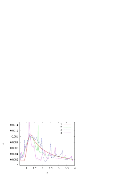
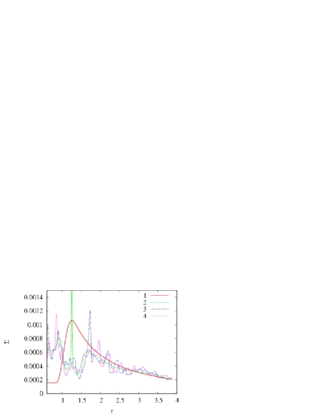
Figure 15: The evolution of the density profiles during the planet migration in a disc with an inner edge. Each panel shows the initial density profile (curve 1), the azimuthal average of the surface density (curve 2; the planet position is visible as a spike) and the surface density cuts through the Lagrange points L5 (curve 3) an L4 (curve 4). The panels upper left, upper right, lower left and lower right show the density profiles after $40$, $50$, $60$ and $70$ orbits, respectively.

In this section we address the processes that stop rapid type III migration. We consider two possible causes. In the first one migration slows down due to the decrease of the volume of the co-orbital region, and in the second one the planet stops at an inner disc edge. When discussing stopping of type III migration we mean a radical slow-down of migration to a rate similar to type II migration, or $|Z|\ll 1$. However, an exact stopping, $Z=0$, can be observed in some cases.

Since the non-dimensional migration rate $Z$ is a function of the co-orbital mass deficit $M_{\mathrm{\Delta}}$, to stop a type III migration we have to diminish $M_{\mathrm{\Delta}}$. This can be achieved by either decreasing the mass of the co-orbital region or by removing the asymmetry in this region. The migration rate depends on the amount of angular momentum transferred between the planet and the gas crossing the planet’s orbit. To start and maintain rapid migration the impulse that the planet gets from the orbit crossing gas has to be strong enough to move the planet into the undisturbed region of the disc where it can interact with a new portion of gas. This impulse depends on the change in the radial position of the gas element crossing the orbit given by $x_{\mathrm{s}}$ and the asymmetry in the co-orbital region given by $\Sigma_{\mathrm{s}}-\Sigma_{\mathrm{g}}$ (Eq. 2). Assuming maximal asymmetry and putting $\Sigma_{\mathrm{g}}=0$ leaves us with two parameters, $\Sigma_{\mathrm{s}}$ and $x_{\mathrm{s}}$, whose product is proportional to the mass of the co-orbital region. This parameter allows us to qualitatively understand the stopping mechanism for type III migration and the dependence of $Z$ on the disc total mass and on $\alpha_{\mathrm{\Sigma}}$. It is however difficult to get quantitative results, since $\Sigma_{\mathrm{g}}$ in practice is not zero, and depends on the migration history.

Our simulations show that fast migration is not allowed in the region where the mass of the co-orbital region $M_{\mathrm{CR}}$ is smaller than the planet mass. Since for $\alpha_{\mathrm{\Sigma}}>-2$ this parameter decreases with decreasing distance to the star, it is easier to start type III migration further out in the disc. The migration rate decreases with distance to the star and thus there will be an inner region where fast migration cannot occur. This means that in most cases the planet will not be able to migrate inward all the way by type III migration. The value of the radius where the planet stops rapid migration depends on the surface density profile and the planet mass. This radius decreases with increasing $\mu_{\mathrm{D}}$ and decreasing $\alpha_{\mathrm{\Sigma}}$. Planets with smaller masses should be able to migrate further in, but with a lower migration rate since $\dot{a}_{\mathrm{f}}\sim M_{\mathrm{P}}^{-2/3}$. Interestingly, this analysis implies that the situation is reversed in discs with steep density profiles, $\alpha_{\mathrm{\Sigma}}<-2$. In this case it is easier to start fast migration close to the star and the inward migrating planet should increase the migration rate with decreasing distance to the star.

$M_{\mathrm{CR}}$ decreases mostly due to the shrinking of the radial extent of the co-orbital region. This can be seen in Fig. 9, where the the azimuthal average of the surface density (curve 2, and the surface density cuts through the L5 (curve 4) an L4 (curve 5) points are plotted. The planet moves through the disc leaving the surface density profile slightly changed (curve 1 is the original density profile). After $30$ and $40$ orbits the strong asymmetry between L5 and L4 that is driving migration is visible. However, this asymmetry disappears after $50$ orbits even though the mass difference between the inner and outer edge of the co-orbital region still exists. The migration stops since the jump in the radial position of gas crossing the co-orbital region is too small to remove a substantial amount of angular momentum from the planet.

The other mechanism for stopping type III migration is the interaction with a steep density change, such as a disc edge. At a significant density jump $M_{\mathrm{CR}}$ will diminish considerably, and asymmetry in the co-orbital region will disappear. Figure 15 shows the evolution of the density profiles in the simulation presented at the end of Sect. 6.4. The upper left, upper right, lower left and lower right panels show the density profiles at $t=40$, $50$, $60$ and $70$ orbits respectively. At these times $Z\approx-2$, $-1.5$, $-0.05$, $0.0$. At $t=70$ orbits the planet is locked in the disc and gap opening has started. The upper left and upper right panels show the density distribution during the fast migration limit $Z<-1$ and are similar to the upper left and upper right panels in Fig. 9. The lower left panel shows the planet interacting with the disc edge. At this time the mass difference between the inner and outer edge of the co-orbital region disappears and the planet gets a positive value of $Z$. However we found this temporary outward migration to be sensitive to the grid resolution (decreasing for higher resolution).

The results show that a Jupiter is massive enough to destroy the initial density jump and fill the inner empty region. That is why when the planet finally settles, the inner and outer disc have almost equal surface densities. This actually prevents the planet from stopping completely. The situation is different for lower mass planets that cannot change significantly the density profile. They can be trapped close to the position of maximum density for a long time and grow slowly (Masset et al., 2006). To have this happen to a Jupiter-mass planet would require an additional mechanism that removes material from the inner disc and keeps the radial density gradient sharp. Such a mechanism would keep the planet at a constant orbit due to the gas flow from the co-orbital region until the horseshoe region has completely cleared. However, if the rate of mass accretion onto the star is too small to fill the co-orbital region and keep a constant gas flow through the co-orbital region the planet would still move away from its position at the disc edge.

In paper III we will encounter two additional mechanisms that can stop type III migration, but which are more evident in the outward migration case.

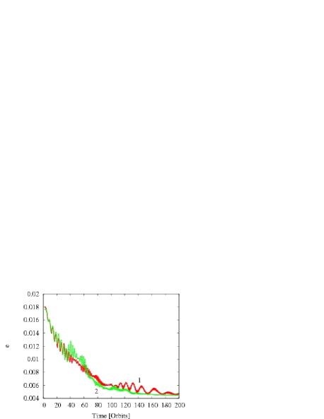
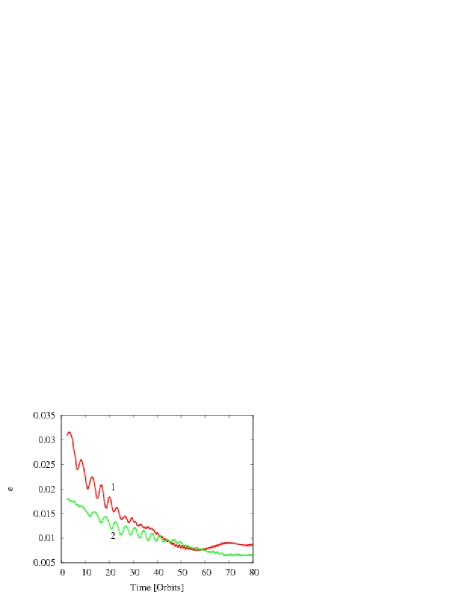
Figure 16: The time evolution of the eccentricity $e$. The left panel shows the results of the models with the constant effective planet’s mass $M_{\mathrm{P}}^{*}=M_{\mathrm{P}}=0.001$ (curve 1) and the model including the gas accretion on the planet (curve 2). The right panel presents the results of the models with different total disc masses. Curves 1 and 2 correspond to $\mu_{\mathrm{D}}$ equal $0.005$ (standard case) and $0.0025$ respectively.

8 Eccentricity evolution

In this section we discuss the eccentricity evolution and its dependency on different simulation parameters. The results of different models are presented in Fig. 16, see also the top right panel of Fig. 1 for our standard case.

The left panel of Fig. 16 shows the time evolution of the eccentricity $e$ for the model with the constant effective planet’s mass $M_{\mathrm{P}}^{*}=M_{\mathrm{P}}=0.001$ (curve 1) and the model including the gas accretion on the planet (curve 2). In the second model the planet’s mass was increased by the gas mass removed from the planet’s proximity (for more discussion see Paper I Sect. 5.1.2). It shows that during the rapid migration phase (lasting for about 70 orbits) the evolution of the eccentricity is almost independent of the planet’s mass and the mass of the circumplanetary disc. The eccentricity grows rapidly during the first few orbits and reaches $0.018$, and diminishes with time on the timescale of migration or faster. The differences between the models show up in the slow migration phase, where the first model loses gas from the Hill sphere and the eccentricity starts to oscillate due to these gas motions in the circumplanetary disc. In the second model accretion has removed most of the mass of the circumplanetary disc, and the eccentricity slowly decays without oscillations. We found similar results in simulations with the $\widetilde{M}_{\mathrm{P}}=M_{\mathrm{P}}+M_{\mathrm{soft}}$ and different initial planet masses $M_{\mathrm{P}}$. In all of these cases the time-scale for the eccentricity damping during the rapid migration phase is independent on the planet mass. We found it to be weakly dependent on other simulation parameters such as the density profile exponent $\alpha_{\mathrm{\Sigma}}$.

However, the time-scale for the eccentricity damping does depends on the total disc mass. The right panel in Fig. 16 shows the time evolution of $e$ for the models with $\mu_{\mathrm{D}}$ equal $0.005$ and $0.0025$ (curves 1 and 2). The value of $e$ after a few first orbits depends on $\mu_{\mathrm{D}}$ and is about $0.03$ and $0.017$ for the first and the second model respectively. In both models the eccentricity is damped during the rapid migration phase, and the corresponding damping time-scale is about $33$ and $69$ orbits. This suggests that the damping time-scale is proportional to $1/\mu_{\mathrm{D}}$

A probable explanation for the eccentricity damping is the presence of dense gas in the region of the strong $e$-damping co-orbital Lindblad resonances. Although the eccentricity driving theory of Artymowicz (1993) does not explicitly account for the modification of gas flow in the corotational region and is not meant for gap-opening planets, it can provide an approximate upper limit to the strength of eccentricity damping by density wave emission at the Lindblad resonances. Eccentricity driving is a result of the competition between external Lindblad resonances and co-orbital Lindblad resonances, the latter being about 3 times stronger than the former. Since type III migration implies that the gap around the planet is asymmetric, let us assume that the mean gas density in the co-orbital resonance region near the planet is reduced by a factor of 2 with respect to the case of a smooth disk, considered by Artymowicz (1993), equivalent to the simplified view of zero gas density in the libration region and unperturbed values elsewhere. Eccentricity damping occurs in direct proportion to the gas density. Therefore, the resulting eccentricity damping timescale should in our standard case be larger than Artymowicz’s estimate by a factor of $(3-1)/(3/2-1)=4$. In a disk with $\mu_{D}=0.005$, $h_{\mathrm{s}}=0.05$ everywhere, and $\alpha_{\Sigma}=-3/2$, we obtain the following lower limit on the damping timescale at $a=5$ AU:

$$e/\dot{e}>(0.008/\mu){\rm yr}$$ (14)

(where $\mu=0.001$ for Jupiter), giving 8 years (about one orbit) at Jupiter’s radius. This is much shorter than the numerically determined timescale for $e$ to drop from $e=0.02718$ to $e=0.01$, which equals about 30 periods, as can be seen in Fig. 1. We conclude that the analytical description is consistent with our calculations but does not provide a good guidance. A theory better adjusted to the corotational gas flow streamlines and/or eccentric corotational torques is needed. It is interesting to note that eccentricity damping and migration can operate on a similar, short timescales.

9 Conclusions

In this paper we presented a study of inward directed type III migration of Jupiter-mass planets embedded in a disc. We used two dimensional numerical simulations, performed in a Cartesian coordinate system and the inertial reference frame. We focused on the detailed flow structure in the planet’s vicinity and used an adaptive mesh refinement to achieve high resolution inside the Roche lobe. We used a modified version of the usual local-isothermal approximation, where the temperature depends on the distance to both the star and the planet, and also added a correction for the gas self-gravity near to the planet.

Type III migration is driven by the co-orbital torque $\Gamma_{\mathrm{CR}}$ exerted on the planet by the gas crossing the co-orbital region. The value of this torque depends on the mass flux crossing the planet’s orbit and on the density asymmetry in the co-orbital region. This asymmetry can be characterised by the non-dimensional migration rate $Z=\dot{a}/\dot{a}_{\mathrm{f}}$ which gives the ratio between the the migration timescale (defined as $x_{\mathrm{s}}/{\dot{a}}$) and libration timescale. We can thus divide type III migration into a slow ($|Z|<1$) and a fast ($|Z|>1$) migration limit. The shape and the structure of the horseshoe region differ between these two limits as the azimuthal extent of the horseshoe region decreases with $|Z|$. In the slow migration limit the horseshoe region fills the whole co-orbital region and the flow asymmetry is limited to the planet’s direct vicinity. Both tadpole regions are present, although their shape changes with $Z$ and the positions of the stationary points move away from the Lagrangian points L4 and L5. In the fast migration limit the whole horseshoe region shrinks to a single tadpole-like region.

In the fast migration limit the planet’s radial motion is too fast to allow a gap to be opened (Fig. 6 and 7). Instead there is a strong gas flow through the corotation region, moving gas from the inner disc (the region with $r<a-x_{\mathrm{s}}$) to the outer disc (the region with $r>a+x_{\mathrm{s}}$). In the inertial reference frame the planet together with the gas captured in the horseshoe region moves fast with respect to the gas that was initially placed in the inner disc (Fig.2). Note that there is no global motion for most of the gas in the disc in this case. Although the fluid captured by the planet in the horseshoe region moves together with the planet, the gas crossing the corotation changes its initial position in the disc only by order of $x_{\mathrm{s}}$. This is an important difference with type II migration, where the planet is locked in the disc and moves on the viscous time scale. In the slow migration limit, when the migration timescale becomes longer than the libration timescale, the planet starts clearing a gap, and gradually makes the transition to type II migration.

Another difference between the slow and fast migration limits is the relation between $\Gamma_{\mathrm{CR}}$ and $Z$. The torque exerted on the planet depends mostly on the structure of the flow lines in the horseshoe region and in the circumstellar disc. In the slow migration limit the flow through the corotation is limited to the a narrow stream at a boundary of the Roche lobe and the asymmetry of both the circumplanetary disc and the horseshoe region is relatively small. This asymmetry is sensitive to the small changes in $Z$, giving a strong dependence of the total torque $\Gamma$ (dominated by the corotational torque) on $Z$. On the other hand in the fast migration limit the asymmetry of the circumplanetary disc and the horseshoe region is significant, the gas can cross the co-orbital region over a wide azimuthal range and the total torque is only weakly dependent on $Z$. This results in a linear grow of the total torque $|\Gamma|$ with $|Z|$ in the slow migration limit and a saturation of $|\Gamma|$ around $Z\approx-1.5$. In the fast migration $|\Gamma|$ decreases slowly with $|Z|$.

The torque also depends on the rate of mass accumulation in the planet’s vicinity, which is related to the non-dimensional migration rate (Fig. 3), and on the assumed scale height for the circumplanetary disc. For $h_{\mathrm{p}}=0.4$ the effective planet mass grows slowly in the fast migration limit, since in this case the horseshoe region contracts into a single tadpole-like region, and most of the fluid crossing the co-orbital region does not enter the Roche lobe. The gas orbits in the circumplanetary disc are found to be strongly asymmetric, and the gas flow into the Roche lobe is limited. The asymmetry of the horseshoe region and the circumplanetary disc diminishes with decreasing $|Z|$, and the mass accumulation rapidly increases for $Z\approx-1.7$. This causes the torque generated inside the Hill sphere to drop significantly and shortly after the planet enters the slow migration limit, where the co-orbital flow is limited to the a narrow stream in the planet’s neighbourhood, and the circumplanetary disc becomes more symmetric. This allows the planet to capture a larger amount of the mass, but this process is limited by the fact that the mass flux crossing the planet orbit decreases quickly with $|Z|$, thus ending the mass accumulation phase close to $Z\approx-0.6$. The fast mass accumulation builds up a strong pressure gradient in the planet’s proximity, which is only supported by the gas inflow into the circumplanetary disc. After the mass accumulation phase ends gas starts to flow away from the circumplanetary disc, and short phase of outward migration can occur.

The growth of the effective planet mass is strongly dependent on the assumed temperature profile in the circumplanetary disc, decreasing for larger circumplanetary disc aspect ratios. For $h_{\mathrm{p}}\geq 0.5$ we found no substantial mass accumulation, and gas is lost from the the planet’s environment during the entire slow migration limit.

The planet mass plays an important role, even though the planet’s orbital evolution is only weakly dependent on it in the fast migration limit. Since $Z\sim\widetilde{M}_{\mathrm{P}}^{-2/3}$, the planet with bigger mass (or lower $h_{\mathrm{p}}$) makes the transition to the slow migration limit sooner, and settle at larger radii than planets with lower mass (or larger $h_{\mathrm{p}}$).

The position where the planet stops rapid type III migration thus depends on the planet’s mass, but also on the disc structure. The mass of the co-orbital region defines the region of the disc where the rapid migration is allowed. To start and maintain type III migration the mass of the co-orbital region has to be comparable to the planet mass. This means that an increase of the disc mass gives a similar effect as a decrease of the planet’s mass.

The planet’s orbital evolution is determined by the changes of the co-orbital mass deficit $M_{\mathrm{\Delta}}$, expressing the mass and the asymmetry of the co-orbital region. The mass is the product of the density profile and the volume of the co-orbital region. For discs with $\alpha_{\mathrm{\Sigma}}>-2$ it therefore decreases with radius, and inward rapid migration always slows down. This is the stopping mechanism for most of the simulations presented in this paper. Type III migration can also be stopped at significant density jumps in the disc (such as a disc edge). In this case the asymmetry of the horseshoe region is lost due to the interaction with the low density region and the planet rapidly makes the transition to the slow migration regime $|Z|\ll 1$.

In all our simulations the eccentricity did not exceed $0.04$ and was damped during the rapid migration phase. We found the damping time-scale to be independent of the planet mass, but inversely proportional to the total disc mass. The measured damping time-scales are few times longer than the one predicted by the analytical formulation.

The results in this paper show that type III migration can operate effectively, but does require the mass in the co-orbital region to be larger than the planet mass in order to get started, making it easier to start type III migration for lower mass planets, and for positions further out in the disk. The mass of the co-orbital region also sets a limit on how far the planet can migrate inward. The minimum orbital radius it can attain is again set by the position where the co-orbital mass exceeds twice the planet mass. It can however stop at larger radii than that, depending on the details of the density structure of the co-orbital region. For all cases the use of the dimensionless migration rate $Z$ is useful to characterise the migration behaviour and the structure of the co-orbital region. Calculating $Z$ can for example be used to check whether type I or type II migration will lead to type III migration.

The simulations presented in this paper were set up to study inward migration in the type III regime. In a real disc-planet interaction, type III migration may also lead to outward migration, this depending on the details of the previous migration pattern. This outward migration mode will be studied in detail in a subsequent paper.

References

- Artymowicz (1993) Artymowicz P., 1993, ApJ, 419, 166
- Artymowicz (2004) Artymowicz P., 2004, in Caroff L., Moon L. J., Backman D., Praton E., eds, Debris Disks and the Formation of Planets Vol. 324 of Astronomical Society of the Pacific Conference Series, Dynamics of Gaseous Disks with Planets. pp 39–+
- Artymowicz (2006) Artymowicz P., 2006, in Daflon S., Alcaniz J., Telles E., de la Reza R., eds, Graduate School in Astronomy: X Vol. 843 of American Institute of Physics Conference Series, Planetary Systems. pp 3–34
- Artymowicz & de Val Borro (2007) Artymowicz P., de Val Borro M., 2007, ApJ, in preparation