QUASINORMAL MODES AND LATE-TIME TAILS OF CANONICAL ACOUSTIC BLACK HOLES

Abstract

abstract

In this paper, we investigate the evolution of classical wave propagation in the canonical acoustic black hole by numerical method and discuss the details of tail phenomenon. The oscillating frequency and damping time scale both increase with the angular momentum $l$. For the lower $l$, numerical results show the lowest WKB approximation gives the most reliable result. We also find that time scale of the interim region from ringing to tail is not affected obviously by changing $l$.

I Introduction

Some properties of black holes can be investigated using acoustic analogues in the laboratory through the propagation of sound wave. Hawking radiation is a remarkable prediction and is almost universally believed to be one of the most important in black hole’s physics. However, the Hawking temperature of astrophysical black holes is much smaller than the temperature of the cosmic microwave background so that one cannot acquire any conclusive evidence of the existence of Hawking radiation. About twenty-five years ago, Unruh proposed a method that certain aspects of astrophysical black hole are mapped into problems in the theory of supersonic acoustic flows EBHE . Even though the Hawking temperatures associated to acoustic analogues are not high enough to be detectable up to now, the situation is likely to change in the near future acoustic . A profound understanding of the classical physics of acoustic black hole is indispensable for the detection of Hawking radiation. Berti, Cardoso and Lemos Berti investigated wave propagation in the “draining bathtub” model and the “canonical” (1+3)-dimensional acoustic black hole Visser . Especially, using the Wentzel-Kramers-Brillouin (WKB) method, they calculated the quasinormal modes (QNMs). Many physicists believe that the figure of QNMs is a significant fingerprint indirectly identifying the existence of a black hole. The QNMs of black holes in the framework of general relativity Cardoso ; Giammatteo and string theory Li ; Xi has been studied widely.

Approximately, there are three stages in the evolution of the perturbations of an acoustic black hole Berti . First stage is the rapid response at very early time, on which the initial conditions have a great effect. Second stage is quasinormal ringing phase, which characteristic oscillation frequencies and damping times depend strongly on the acoustic analogue QNMs. The QNMs are determined completely by the parameters of system, therefore they would carry significant information about the background curvature of the intervening spacetime. Finally, there is a tail stage, which decays approximately as a power in time owing to backscattering off the spacetime curvature. In Ref. 3, the authors have used three WKB computational schemes, i.e. the lowest approximation Will , 3rd order improvements Iyer ; Seidel and 6th order corrections Konoplya . For the canonical acoustic black hole, the results show that $l=1$ QN frequencies seem to be the problem, in which the mode suffers a large variation as one goes from the lower approximation to the higher approximation. This means that the WKB approach is more dependable for higher $l$, which was first discovered in the early work Will ; Iyer ; Seidel . Therefore, the numerical calculation is necessary for the lower $l$ QN frequencies.
In this paper, we investigate in detail the relations between QNMs of canonical acoustic black hole and the angular momentum $l$ by the numerical calculation in null coordinates. Some results attained by this way are supported by the analytic results and WKB results. Most of importance, we confirm that the lowest WKB approximation gives the most reliable results for $l=1$ case. Furthermore, we show a picture of classical wave propagation including the interim region from the quasinormal ringing to tail stage.

II FORMALISM AND BASIC EQUATIONS

Assume the fluid to be incompressible and spherically symmetric, then since background density $\rho$ is position independent the continuity equation implies the velocity is in proportion to $r^{-2}$. The background pressure $p$ and speed of sound $c$ are also position independent because of the barotropic assumption. Therefore, one can define a normalization constant $r_{0}\equiv\left({vr^{2}/c}\right)^{{\frac{{1}}{{2}}}}$. The canonical acoustic metric describing the propagation of sound waves in this incompressible and spherically symmetric (1+3)-dimensional fluid flow Visser is:

$$ds^{2}=-c^{2}\left({1-{\frac{{r_{0}^{4}}}{{r^{4}}}}}\right)dt^{2}+\left({1-{\frac{{r_{0}^{4}}}{{r^{4}}}}}\right)^{-1}dr^{2}+r^{2}(d\theta^{2}+\sin^{2}\theta d\phi^{2})$$ (1)

The metric (1) is distinct from any of the geometries typically considered in general relativity. Unruh EBHE first suggested that the propagation of a sound wave is described by the Klein-Gordon equation $\nabla_{\mu}\nabla^{\mu}\Psi=0$ for a massless scalar field $\Psi$ in a Lorentzian acoustic geometry, which take metric (1) at present. We can separate variables by setting

$$\Psi(t,r,\theta,\phi)={\frac{{1}}{{r}}}\Phi(r_{\ast},t)Y_{lm}(\theta,\phi)$$ (2)

where $Y_{lm}(\theta,\phi)$ are the usual spherical harmonics and the tortoise coordinate $r_{\ast}$ is defined by

$$r_{\ast}={\int{(1-{\frac{{r_{0}^{4}}}{{r^{4}}}})^{-1}dr}}$$ (3)

where we have chosen unit $c=1$. The evolution equation of $\Phi(r_{\ast})$ is

$${-\frac{{\partial^{2}\Phi}}{{\partial t^{2}}}+\frac{{\partial^{2}\Phi}}{{\partial r_{\ast}^{2}}}}=V\Phi$$ (4)

where the effective potential

$$V(r_{\ast})=(1-{\frac{{r_{0}^{4}}}{{r^{4}}}})[{\frac{{l(l+1)}}{{r^{2}}}}+{\frac{{4r_{0}^{4}}}{{r^{6}}}}]$$ (5)

We introduce the null coordinates $u=t-r_{\ast}$ and $v=t+r_{\ast}$, Eq. (5) can be reduced to

$$-4{\frac{{\partial^{2}\Phi}}{{\partial u\partial v}}}=V(r_{\ast})\Phi$$ (6)

Eq. (6) can be numerically integrated by the ordinary finite element method. Using the Taylor expansion, we have

$$\Phi_{N}=\Phi_{E}+\Phi_{W}-\Phi_{S}-\delta u\delta v(\frac{v_{N}+v_{W}-u_{N}-u_{E}}{4})\frac{\Phi_{W}+\Phi_{E}}{8}V(r_{\ast})+O(\Delta^{4})$$ (7)

where $N$, $W$, $E$ and $S$ are the points of a unit grid on the $u-v$ plane which correspond to ($u+\Delta$,$v+\Delta$ ),($u+\Delta$,$v$),($u$,$v+\Delta$) and ($u$, $v$), and $\Delta$ is the step length of the change of $u$ or $v$, i.e., $\Delta=\delta u=\delta v$ Li ; Xi . Because the quasinormal ringing stage and the late time stage are both insensitive to the initial conditions, we begin with a Gaussian pulse of width $\sigma$ centred on $v_{c}$ when $u=u_{0}$ and set the field $\Phi$ is zero on $v=v_{0}$,

$$\Phi(u=u_{0},v) = exp[-{\frac{{(v-v_{c})^{2}}}{{2\sigma^{2}}}}]$$

$$\Phi(u,v=v_{0}) = 0$$ (8)

Next, the point in the $u-v$ plane can be calculated by using Eq. (6), successively. Finally, the values of $\Phi(u_{max},v)$ are extracted after the integration is completed where $u_{max}$ represents the maximum of $u$. Taking sufficiently large $u_{max}$ for the various $v$-value, we obtain a good approximation for the wavefunction of canonical acoustic black hole.

III NUMERICAL RESULTS

Our numerical results, which are all consistent with the analytic results and WKB results in Ref. 3, are shown in Figs. 1-6. As a reminder, the oscillating period, damping time scale and late time tail are shown in these figures. Here, the parameter $r_{0}$ is set to uninty. The dependence of quasinormal modes on $r_{0}$ is trivial. On the one hand, the canonical acoustic metric coordinates can be rescaled to set $r_{0}=1$. On the other hand, the results must depend linearly on $r_{0}$ since it is the only dimensional quantity in the problem. In Fig. 1, we show the relations between the wavefunction and the angular momentum $l$. Our numerical result is consistent with Ref. 3. That means the oscillating period and the damping frequency both decrease when the index $l$ increases. Furthermore, we confirm that the lowest WKB approximation gives the most reliable results for $l=1$ case. To further corroborate this conclusion, we list QN frequencies for $l=1,2,3,4$ in Table 1.

QN frequencies of the canonical acoustic black hole for $l=1,2,3,4$ are listed.
$l$ $Re(\omega)$ $Im(\omega)$ 10 01.463 00.666 20 01.619 00.653 30 01.642 00.625 40 01.758 00.620

In Figs. 2-6, we choose $l=2$, and consider in detail the picture of classical wave propagation in the canonical three stages, the second and final stages as illustrated in Fig. 2. The prompt contribution is the evident counterpart of light cone propagation in the $V=0$ case, which strongly depends on the initial conditions, therefore it is left out in Fig. 2. At intermediate $v$ values the wavefunction is dominated by an exponential decay, whose oscillation frequency and damping time are described by its QNMs. At the late-time (large $v$ value) the propagating wave leaves a power-law tail which is magnified in Fig. 3. By numerical calculation, we attain the expression of power-law falloff, $\Phi\approx 7.36\times 10^{-32}t^{-10}$, which is consistent with the analytic result in Ref. 3. Especially, the interim region from ringing stage to tail stage is corresponding to rectangular region A in Fig. 2. This interim region is replotted in Fig. 4, where the $v$-coordinate is magnified about $10^{3}$ times. The time interval from region B to region C is so short that the numerical results between region B and region C seem unfaithful. Therefore, we do not discuss physical implications about this region, attentively. The rectangular regions B and C of Fig. 4 are magnified in Fig. 5 and Fig. 6, respectively. In region B, the oscillation frequency dramatically changes and tends to zero. Likewise, in region C, the damping time scale also has a drastic change, which becomes infinity. These figures tell us how perturbation in vicinities of this black hole die out as a late-time tail. It is easy to find that time scale of interim region from ringing to tail is not affected obviously by changing the angular momentum $l$.

Figure 1: For the canonical acoustic black hole with $r_{0}=1$, the wavefunctions are shown via different the angular momentum $l$. The logarithm is to base 10.

Figure 2: For the canonical acoustic black hole with $r_{0}=1$ and $l=2$, the rectangular region A describes as interim region from ringing to tail. The logarithm is to base 10.

Figure 3: The late-time tail in Fig. 2 is magnified. The logarithm is to base 10.

Figure 4: For the canonical acoustic black hole with $r_{0}=1$ and $l=2$, the interim region from ringing to tail is shown.

Figure 5: The rectangular region B in Fig. 4 is magnified. The logarithm is to base 10.

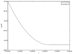
Figure 6: The rectangular region C in Fig. 4 is magnified. The logarithm is to base 10.

IV CONCLUSIONS

In this work we considered numerically the evolution of classical wave propagation in the canonical acoustic black hole and discussed the details of tail phenomenon. We summarize main results as follows:
(i) For $l\geq 2$, the numerical results are consistent with the first, third and sixth order WKB method. For the lower $l$, numerical results show the first WKB approximation gives the most reliable result because of the basic WKB assumption (the ratio of the derivatives of the potential to the potential itself should be small) is broken.
(ii) From a physical viewpoint, the most reasonable explanation for the production of late-time tails is the backscattering of waves off a spacetime curvature at asymptotically far regions. Our numerical results show that late-time tail is consistent with Ref. 13, and time scale of the interim region from ringing to tail is not affected obviously by changing the angular momentum $l$.
(iii) The oscillating frequency and damping time scale both increase with the angular momentum $l$. In the limit of large $l$, the real part of fundamental QN frequency increase linearly and imaginary part tend to a constant with the angular momentum $l$.

References

W. G. Unruh, Phys. Rev. Lett. 46, (1981) 1351.

R. Schützhold and W. G. Unruh, Phys. Rev. Lett. 95, (2005) 031301.

E. Berti, V. Cardoso and J. P. S. Lemos, Phys. Rev. D70, (2004) 124006.

M. Visser, Class. Quantum Grav. 15, (1998) 1767.

V. Cardoso, J. P. S. Lemos and S. Yoshida, Phys. Rev. D69, (2004) 044004.

M. Giammatteo and I. G. Moss, Class. Quantum Grav. 22, (2005) 1803.

X. Z. Li, J. G. Hao and D. J. Liu, Phys. Lett. B507, (2001) 312.

P. Xi and X. Z. Li, Chin. Phys. Lett. 22, (2005) 2763.

B. F. Schutz and C. M. Will, Astrophys. Journal 291, (1985) L33.

C. M. Will and S. Iyer, Phys. Rev. D35, (1987) 3621.

E. Seidel and S. Iyer, Phys. Rev. D41, (1990) 374.

R. A. Konoplya, Phys. Rev. D68, (2003) 024018.

E. S. C. Ching, P. T. Leung, W. M. Suen and K. Young, Phys. Rev. D52, (1995) 2118.