Flatness-based pre-compensation
of laser diodes .

Abstract

A physical nonlinear dynamical model of a laser diode is considered. We propose a feed-forward control scheme based on differential flatness for the design of input-current modulations to compensate diode distortions. The goal is to transform without distortion a radio-frequency current modulation into a light modulation leaving the laser-diode and entering an optic fiber. We prove that standard physical dynamical models based on dynamical electron and photons balance are flat systems when the current is considered as control input, the flat output being the photon number (proportional to the light power). We prove that input-current is an affine map of the flat output, its logarithm and their time-derivatives up to order two. When the flat output is an almost harmonic signal with slowly varying amplitude and phase, these derivatives admit precise analytic approximations. It is then possible to design simple analogue electronic circuits to code approximations of the nonlinear computations required by our flatness-based approach. Simulations with the parameters of a commercial diode illustrate the practical interest of this pre-compensation scheme and its robustness versus modelling and analogue implementation errors.

1 Introduction

Radio-over-Fiber is a very attractive technique for wireless access network infrastructure, because it can transmit microwaves and millimeter-waves through optical fibers for a long distance. Therefore, the distribution of radio signals over optical fiber, which is of great interest for many applications such as broad-band wireless access networks, sensor networks, radar and satellite communications, has been intensively studied. And there have been rapid advances in the techniques to generate and transport radio signals over optical fiber in recent years (see, e.g., [2]). When the wireless channel is in series with the optical link, nonlinear distortion due to the electrical/optical conversion is the biggest concern (see, e.g., [7]). This makes nonlinearity compensation an attractive solution to improve link performance.

The focus of this work is to investigate the standard physical model used for describing commercial laser diodes. This model is based on rate equation for the electron and photon populations. This allows us to propose a pre-compensation based on differential flatness for the design of the input current in order to cancel diode distortions. Simulations corresponding to a commercial laser diode illustrate the pre-compensation scheme. When the distortion due to the optic fiber is negligible, our flatness-based pre-compensation scheme can be interesting to increase the bandwidth and transmission rate.

This paper is organized as follows. In section 2 we recall the standard diode model and show that it is structurally flat, with the photon number being the flat output $y$. We show via elementary computations that the input current is a linear combination of $y$, ${\frac{d}{dt}}y$, ${\frac{d^{2}}{dt^{2}}}y$, ${\frac{d}{dt}}(\log y)$ and ${\frac{d^{2}}{dt^{2}}}(\log y)$ with coefficients depending via explicit formula on the physical parameters (equation (3)). This relation is the starting point of the flatness based pre-compensation scheme addressed in section 3. In Section 4, we propose natural approximations when $y$ is quasi-harmonic with slowly varying amplitude and phase. These approximations simplify considerably the computation burden in such a way that a nonlinear analogue circuit can be easily design to realize our flatness-based pre-compensation scheme. In conclusion, we propose some hint to deal with phase influence that becomes important when fiber distortions cannot be negligible.

2 The flat physical nonlinear model

A standard nonlinear model relating the input-current $I$ to the power of the emitted light $P$ is recalled in [5] where this model is used to analyze the nonlinear ”transfer” between input-current modulation $I$ and the resulting output $P$) (see also [1] for a simple exposure on such basic models):

$$\left\{\begin{aligned} {\frac{d}{dt}}P&=R(P,X)-\frac{P}{\tau_{p}}\\ {\frac{d}{dt}}X&=\frac{I}{I_{th}\tau_{n}}-\frac{X}{\tau_{n}}-aR(P,X)\end{aligned}\right.$$ (1)

where

• $\tau_{p}$ and $\tau_{n}$ are photon and carrier lifetimes;

• $X$ is the normalized carrier density;

• $I_{th}$ is the threshold current and $a$ is the constant related to other physical parameters, $a=FI_{th}\tau_{n}/\tau_{p}$.

• $R(P,X)$ is the net rate of stimulated emission. Following [5] we use

  $$R(P,X)=\left(\frac{B\tau_{n}I_{th}(X-1)+\frac{1}{\tau_{p}}}{1+FB\tau_{p}\tau_{c}P}\right)P$$

  where $B$, $\tau_{n}$,$\tau_{c}$ are physical parameters .

Since the input-current appears only in the second differential equation of (1) (the electron balance equation), the first state, $P$, is a flat output. More precisely, this means that, if we consider (1) as a control system with input $I$ and output $y=P$, we have a nonlinear input/output system such that its inverse admits no dynamics. This system is differentially flat (see [3, 4, 6, 8]) with $P$ as flat output: the input $I$ is a nonlinear function of $P$, ${\frac{d}{dt}}P$, ${\frac{d^{2}}{dt^{2}}}P$. Notice that this property is independent of the precise form of $R(P,X)$ when it depends effectively on $X$. This is always the case for physical reasons.

Let us detail now the computations with the precise form of $R$ given here above. The first equation of (1) yields

$$X=1+\frac{P}{P_{l}}+\tau_{p}{\frac{d}{dt}}\left(\frac{P}{P_{l}}\right)+\tau_{l}{\frac{d}{dt}}\log\left(\frac{P}{P_{l}}\right)$$

where $P_{l}=\frac{I_{th}\tau_{n}}{F\tau_{c}}$ and $\tau_{l}=\frac{1}{B\tau_{n}I_{th}}$ are constant parameters. Thus we can derive this expression versus $t$ to get ${\frac{d}{dt}}X$ as a function of $P$, ${\frac{d}{dt}}P$ and ${\frac{d^{2}}{dt^{2}}}P$:

$${\frac{d}{dt}}X={\frac{d}{dt}}\left(\frac{P}{P_{l}}\right)+\tau_{p}{\frac{d^{2}}{dt^{2}}}\left(\frac{P}{P_{l}}\right)+\tau_{l}{\frac{d^{2}}{dt^{2}}}\log\left(\frac{P}{P_{l}}\right)$$

A linear combination of the two equations of (1) gives $I$ explicitly:

$$\frac{I}{I_{th}}=X+\tau_{n}\dot{X}+\frac{F\tau_{p}}{\tau_{n}I_{th}}(\dot{P}+P/\tau_{p}).$$

Thus we have the explicit formula relating $I$ to the derivatives of $P$:

$$\frac{I}{I_{th}}=1+\left(1+\frac{\tau_{n}}{\tau_{c}}\right)\left(\frac{P}{P_{l}}\right)+\left(\tau_{n}+\tau_{p}+\frac{\tau_{n}\tau_{p}}{\tau_{c}}\right){\frac{d}{dt}}\left(\frac{P}{P_{l}}\right)\\ +\tau_{n}\tau_{p}{\frac{d^{2}}{dt^{2}}}\left(\frac{P}{P_{l}}\right)+\tau_{l}\left({\frac{d}{dt}}\log\left(\frac{P}{P_{l}}\right)+\tau_{n}{\frac{d^{2}}{dt^{2}}}\log\left(\frac{P}{P_{l}}\right)\right)$$

With the normalized input/ouput variables

$$u=\frac{I}{I_{th}},\quad y=\frac{P}{P_{l}}=\frac{P}{\frac{I_{th}\tau_{n}}{F\tau_{c}}}$$ (2)

we have the following simple but nonlinear input/output relationships that is equivalent to the physical model (1):

$$u=1+\left(1+\frac{\tau_{n}}{\tau_{c}}\right)y+\left(\tau_{n}+\tau_{p}+\frac{\tau_{n}\tau_{p}}{\tau_{c}}\right){\frac{d}{dt}}y\\ +\tau_{n}\tau_{p}{\frac{d^{2}}{dt^{2}}}y+\tau_{l}\left({\frac{d}{dt}}(\log y)+\tau_{n}{\frac{d^{2}}{dt^{2}}}(\log y)\right)$$ (3)

where the four parameters $\tau_{n}$, $\tau_{p}$, $\tau_{c}$ and $\tau_{l}=\frac{1}{B\tau_{n}I_{th}}$ are positive time-scales. Remember that the normalized electron density $X$ is a combination of $y$ and ${\frac{d}{dt}}y$:

$$X=1+y+\tau_{p}{\frac{d}{dt}}y+\tau_{l}{\frac{d}{dt}}(\log y).$$

3 Flatness-based pre-compensation

We can now use (3) for deriving feed-forward strategy in order to compensate the non-linear distortion due to the diode. Assume that our goal is to transfer the amplitude and phase modulated signal $\epsilon(t)\cos(\omega t+\phi(t))$ from the current to the light leaving the diode. Here $\omega$ is the carriage pulsation, typically around a few Ghz for radio frequencies, and $\epsilon(t)$ and $\phi(t)$ are slowly varying amplitude and phase where the bits are encoded. This means that $\left|{\frac{d}{dt}}\epsilon\right|\ll\omega\epsilon$ and $\left|{\frac{d}{dt}}\phi\right|\ll\omega$. Without lost a generality, we can assume that $\epsilon<1$. Assume finally that this modulated signal has to be converted in photons $y>0$ according to $y=\bar{y}(1+\epsilon(t)\cos(\omega t+\phi(t)))$ where $\bar{y}$ is some positive constant. This means that our goal is to find the current $u$ leading to such $y$. If one knows the diode parameters we can use (3) to compute $u$.

We have tested in simulation this simple pre-compensation scheme for the commercial diode considered in [5]. For this diode, we have

$$\tau_{n}=179~{}ps,\quad\tau_{p}=4.33~{}ps,\quad\tau_{c}=3.18~{}ps,\quad\tau_{l}=1.81~{}ps.$$

We choose a modulation frequency $\omega$ of $10$ Ghz ($\omega=2\pi 10^{10}~{}s^{-1}$), $\phi=0$ and

$$\epsilon(t)=\frac{1}{5}\left(1-\cos\left(\frac{\omega t}{10}\right)\right).$$ (4)

The average normalized light power is $\bar{y}=0.0175$ corresponds physically to $\bar{P}=1.4$ mW since $P_{l}=78.5$ mW. The simulations of figure 1 illustrate the interest of taking into account the derivative terms in (3) to modulate the input current $u$.

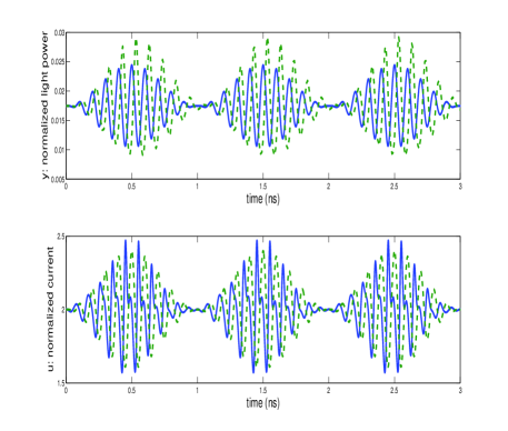
Figure 1: Input current modulations with $\epsilon(t)$ given by (4): the solid curve corresponds to the response of the diode when $u$ is related to $y=\bar{y}(1+\epsilon(t)\cos(\omega t))$ via (3); dashed line corresponds to the response of the diode when $u=1+\left(1+\frac{\tau_{n}}{\tau_{c}}\right)\bar{y}(1+\epsilon(t)\cos(\omega t))$ (static model).

4 Analogue implementation issues

For such high carrier frequency $\omega\sim 10$ GHz, it is difficult and almost impossible to use real-time numerical computations. Let us now propose two approximations such that the above pre-compensation scheme can be applied in real-time via a specific electronic circuit.

The first approximation is relative to the computation of derivative of $y$. Since we are looking for $u$ such that $y=\bar{y}(1+\epsilon(t)\cos(\omega t+\phi(t))$ with $\epsilon$ and $\phi$ slowly varying quantities, we have

$${\frac{d}{dt}}y\approx-\bar{y}\epsilon\omega\sin(\omega t+\phi),\qquad{\frac{d^{2}}{dt^{2}}}y\approx-\bar{y}\epsilon\omega^{2}\cos(\omega t+\phi).$$ (5)

The second approximation is relative to the nonlinearity attached to the $\log$-terms in (3). Now we will use $\epsilon\ll 1$ and propose an approximation up to second order terms:

$${\frac{d}{dt}}(\log y) \approx-\epsilon\omega\sin(\omega t+\phi)(1-\epsilon\cos(\omega t+\phi))$$

$${\frac{d^{2}}{dt^{2}}}(\log y) \approx-\epsilon\omega^{2}(\cos(\omega t+\phi)+\epsilon(2\sin^{2}(\omega t+\phi)-1))$$ (6)

Plugging these approximations into (3) shows that $u$ can be expressed approximatively as a polynomial of degree $2$ in $\epsilon\sin(\omega t+\phi)$ and $\epsilon\cos(\omega t+\phi)$. Such polynomial computations can be easily done by a nonlinear analogue circuit. Figure 2 shows that the diode response remains almost the same when such polynomial approximations are used. Other simulations displayed on figure 3 show that such pre-compensation scheme are also robust to parameters uncertainties.

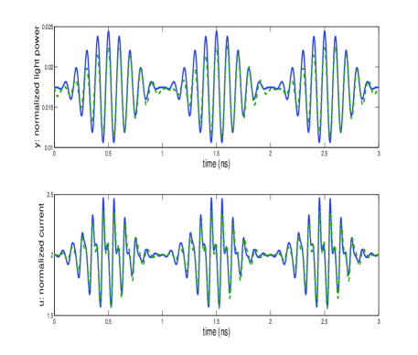
Figure 2: Input current modulations with $\epsilon(t)$ given by (4): the solid curve corresponds to the response of the diode when $u$ is perfectly related to $y=\bar{y}(1+\epsilon(t)\cos(\omega t))$ via (3); dashed line corresponds to the response of the diode when approximations (5) and (6) are used in (3).

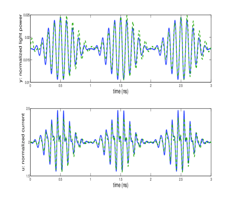
Figure 3: Input current modulations with $\epsilon(t)$ given by (4): as for figure 2, the solid curve corresponds to the response of the diode when $u$ is perfectly related to $y=\bar{y}(1+\epsilon(t)\cos(\omega t))$ via (3); dashed line corresponds to approximations (5) and (6) plugged in (3) but, contrarily to figure 2, the carrier lifetime $\tau_{n}$ used for the computations of the diode response is multiplied by $2$ in order to test robustness versus large parametric errors.

5 Conclusion

We have shown that it is possible to compute, via flatness-based motion planing techniques, adapted input current modulations in order to generate, in real-time and via analogue nonlinear circuits, a given modulation of the light entering the optic fiber. If the distortion along the fiber is not negligible (long fiber and/or refractive index strongly dependent versus optic frequency), we have to consider also the phase dynamic of the light emitted by the diode (see, e.g., [1] for more details about the spectrum widening due to phase/amplitude variations). Following [5] we have to complete (1) by

$${\frac{d}{dt}}\varphi=\frac{\alpha B\tau_{n}I_{t}h}{2}(X-1)$$

where $\varphi$ is the phase of the emitted light and $\alpha$ a positive constant. Thus the emitted light entering the optic fiber is represented by the classical electric field (complex notations)

$$E(t)\propto\sqrt{P(t)}\exp(-\imath\varphi(t))\exp(-\imath\omega_{0}t)$$

where $\omega_{0}$ is the optical frequency (around $10^{15}$ Hz). It is interesting to notice that the diode dynamics (described by three states $(P,X,\varphi)$) and one input $I$) is still flat with $z=\log P+FB\tau_{p}\tau_{c}P-\frac{2}{\alpha}\varphi$ being the new flat output. This results from ${\frac{d}{dt}}z=-\frac{1+FB\tau_{p}\tau_{c}P}{\tau_{p}}$. This structural property could certainly be exploited in other pre-compensation schemes taking into account such additional phase effect.

References

- Agrawal [1997] G.P. Agrawal. Fiber-Optic Communication Systems. John Wiley and Sons, 1997.
- Ai-Raweshidy and Komaki [2002] H. Ai-Raweshidy and S. Komaki. Radio Over Fiber Technologies for Mobile Communications Networks. Artech House, Boston, 2002.
- Fliess et al. [1992] M. Fliess, J. Lévine, Ph. Martin, and P. Rouchon. Sur les systèmes non linéaires différentiellement plats. C.R. Acad. Sci. Paris, I–315:619–624, 1992.
- Fliess et al. [1995] M. Fliess, J. Lévine, Ph. Martin, and P. Rouchon. Flatness and defect of nonlinear systems: introductory theory and examples. Int. J. Control, 61(6):1327–1361, 1995.
- Lee et al. [2003] K.-H. Lee, H.-Y. Choi, and W.-Y. Choi. Analysis of chromatic dispersion-induced second-harmonic distortions including laser dynamics to the second order. IEEE J. of Qauntum Electronics, 39(5), 2003.
- Martin et al. [2003] Ph. Martin, R. Murray, and P. Rouchon. Flat systems, equivalence and trajectory generation, 2003. Technical Report http://www.cds.caltech.edu/reports/.
- Maury et al. [1997] G. Maury, A. Hilt, T. Berceli, B. Cabon, and A. Vilcot. Microwave-frequency conversion methods by optical interferometer and photodiode. IEEE Trans. Microw. Theory Tech., 45:1481–1485, 1997.
- Sira-Ramirez and Agarwal [2004] H. Sira-Ramirez and S.K. Agarwal. Differentially flat systems. CRC, 2004.