NEGATIVE REFLECTION IN A FARADAY CHIRAL MEDIUM

Tom G. Mackay¹ and Akhlesh Lakhtakia²

¹ School of Mathematics
University of Edinburgh
Edinburgh EH9 3JZ, United Kingdom

² CATMAS — Computational & Theoretical Materials Sciences Group
Department of Engineering Science & Mechanics
212 Earth & Engineering Sciences Building
Pennsylvania State University, University Park, PA 16802–6812

ABSTRACT: The four wavenumbers associated with planewave propagation in a Faraday chiral medium (FCM) with relatively huge magnetoelectric coupling give rise to enhanced possibilities for negative–phase–velocity propagation and therefore negative refraction. They can also give rise to the phenomenon of negative reflection. In particular, for a nondissipative example, we deduced that an incident plane wave with positive/negative phase velocity can result in a negatively reflected plane wave with negative/positive phase velocity, as well as a positively reflected plane wave with positive/negative phase velocity.

Keywords: Faraday chiral medium; isotropic chiral medium; negative reflection; negative refraction; negative phase velocity

1. INTRODUCTION

The scope for exotic — and potentially useful — electromagnetic phenomenons to arise is greatly extended in anisotropic mediums, and especially bianisotropic mediums, as compared with isotropic mediums [1, 2]. This letter concerns a particular bianisotropic medium called a Faraday chiral medium (FCM). FCMs combine natural optical activity (as exhibited by isotropic chiral mediums [3]) with Faraday rotation (as exhibited by gyrotropic mediums [4, 5]). They may be theoretically conceptualized as homogenized composite mediums arising from the blending together of isotropic chiral mediums with either magnetically biased ferrites [6] or magnetically biased plasmas [7]. Accordingly, a wide range of constitutive parameters for FCMs may be envisaged.

In a recent study, we identified the propensity of FCMs to support planewave propagation with negative phase velocity, particularly when the magnetoelectric constitutive parameters are relative large [8]. Similar behavior in isotropic chiral mediums and their nonreciprocal counterparts can be traced back to 1986 [9], but is only nowadays being considered carefully [10, 11], following the successful exhibition of the phenomenon of negative refraction by isotropic achiral materials [12]. In the following sections we consider the phenomenon of negative reflection in FCMs. Negative reflection has previously been described for isotropic chiral mediums [13, 14] and anisotropic dielectric mediums [15], but not to our knowledge for bianisotropic mediums.

In the following sections, an $\exp(-i\omega t)$ time dependence is assumed; the permittivity and permeability of free space are denoted by $\epsilon_{0}$ and $\mu_{0}$, respectively; 3–vectors are underlined, with the caret ($\,\hat{}\,$) denoting a unit vector; and 3$\times$3 dyadics are double underlined.

2. PLANEWAVE PROPAGATION

In preparation for solving a boundary–value problem in Section 3, let us consider planewave propagation in a FCM characterized by the frequency–domain constitutive relations [16, 17]

$$\left.\begin{array}[]{l}{\underline{D}}({\underline{r}})=\underline{\underline{\epsilon}}\mbox{ \tiny{${}^{\bullet}$} }{\underline{E}}({\underline{r}})+\underline{\underline{\xi}}\mbox{ \tiny{${}^{\bullet}$} }{\underline{H}}({\underline{r}})\\[5.0pt] {\underline{B}}({\underline{r}})=-\underline{\underline{\xi}}\mbox{ \tiny{${}^{\bullet}$} }{\underline{E}}({\underline{r}})+\underline{\underline{\mu}}\mbox{ \tiny{${}^{\bullet}$} }{\underline{H}}({\underline{r}})\end{array}\right\},$$ (1)

with constitutive dyadics

$$\left.\begin{array}[]{l}\underline{\underline{\epsilon}}=\epsilon_{0}\left[\,\epsilon\,\underline{\underline{I}}-i\epsilon_{g}\,\hat{{\underline{u}}}\times\underline{\underline{I}}+\left(\,\epsilon_{z}-\epsilon\,\right)\,\hat{{\underline{u}}}\,\hat{{\underline{u}}}\,\right]\\ \vspace{-2mm}\\ \underline{\underline{\xi}}=i\sqrt{\epsilon_{0}\mu_{0}}\,\left[\,\xi\,\underline{\underline{I}}-i\xi_{g}\,\hat{{\underline{u}}}\times\underline{\underline{I}}+\left(\,\xi_{z}-\xi\,\right)\,\hat{{\underline{u}}}\,\hat{{\underline{u}}}\right]\\ \vspace{-2mm}\\ \underline{\underline{\mu}}=\mu_{0}\left[\,\mu\,\underline{\underline{I}}-i\mu_{g}\,\hat{{\underline{u}}}\times\underline{\underline{I}}+\left(\,\mu_{z}-\mu\,\right)\,\hat{{\underline{u}}}\,\hat{{\underline{u}}}\,\right]\end{array}\right\}.$$ (2)

Simplifying for the sole purpose of exemplifying negative reflection, we choose the distinguished axis of the FCM to coincide with the $z$ axis; i.e., $\hat{{\underline{u}}}=\hat{{\underline{z}}}$.

Let us also confine ourselves to propagation in the $xz$ plane. Plane waves with field phasors

$$\left.\begin{array}[]{l}{\underline{E}}({\underline{r}})=A\,{\underline{E}}_{\,0}\,\exp\left(i{\underline{k}}\mbox{ \tiny{${}^{\bullet}$} }{\underline{r}}\right)\\[5.0pt] {\underline{H}}({\underline{r}})=A\,{\underline{H}}_{\,0}\,\exp\left(i{\underline{k}}\mbox{ \tiny{${}^{\bullet}$} }{\underline{r}}\right)\end{array}\right\}$$ (3)

can propagate in the FCM, where $A$ is a complex–valued amplitude and the wave vector

$${\underline{k}}=\kappa\,\hat{{\underline{x}}}+\sqrt{k^{2}-\kappa^{2}}\,\hat{{\underline{z}}}=k\,\hat{{\underline{k}}}=k(\hat{{\underline{x}}}\sin\psi+\hat{{\underline{z}}}\cos\psi)$$ (4)

contains the real–valued quantity $\kappa$ that is fixed by the incidence conditions in Section 3. The angle $\psi$ is defined in the clockwise sense with respect to the $+z$ axis in the $xz$ plane.

In order to determine ${\underline{k}}$, ${\underline{E}}_{\,0}$, and ${\underline{H}}_{\,0}$, we substitute (3) in the Maxwell curl postulates $\nabla\times{\underline{E}}({\underline{r}})=i\omega{\underline{B}}({\underline{r}})$ and $\nabla\times{\underline{H}}({\underline{r}})=-i\omega{\underline{D}}({\underline{r}})$, and then use the constitutive relations of the FCM. In general, we find four independent wavevectors for a specific $\kappa$ — namely,

$${\underline{k}}_{j}=\kappa\,\hat{{\underline{x}}}+\sqrt{k_{j}^{2}-\kappa^{2}}\,\hat{{\underline{z}}}=k_{j}(\hat{{\underline{x}}}\sin\psi_{j}+\hat{{\underline{z}}}\cos\psi_{j})\,,\qquad j\in\left[1,4\right],$$ (5)

Corresponding to each ${\underline{k}}_{j}$, there exist ${{\underline{E}}}_{\,0j}$ and ${{\underline{H}}}_{\,0j}=\underline{\underline{\mu}}^{-1}\mbox{ \tiny{${}^{\bullet}$} }\left[(1/\omega)\left({\underline{k}}_{j}\times\underline{\underline{I}}\,\right)+\underline{\underline{\xi}}\right]\mbox{ \tiny{${}^{\bullet}$} }{\underline{E}}_{\,0j}$. Thus, for the purposes of Section 3, the complete representation of plane waves in the FCM for a specified $\kappa$ is

$$\left.\begin{array}[]{l}{\underline{E}}({\underline{r}})=\sum_{j=1}^{4}\,A_{j}\,{\underline{E}}_{\,0j}\,\exp\left(i{\underline{k}}_{j}\mbox{ \tiny{${}^{\bullet}$} }{\underline{r}}\right)\\[5.0pt] {\underline{H}}({\underline{r}})=\sum_{j=1}^{4}\,A_{j}\,{\underline{H}}_{\,0j}\,\exp\left(i{\underline{k}}_{j}\mbox{ \tiny{${}^{\bullet}$} }{\underline{r}}\right)\end{array}\right\}\,,$$ (6)

wherein we have neglected the remote possibility of the existence of Voigt waves [18].

The associated time–averaged Poynting vector is given by

$${\underline{P}}({\underline{r}})=\sum_{j=1}^{4}\,{\underline{P}}_{j}({\underline{r}})=\frac{1}{2}\sum_{j=1}^{4}\,|A_{j}|^{2}\,\mbox{Re}\,\left(\,{\underline{E}}_{\,0j}\times{\underline{H}}_{\,0j}^{*}\,\right)\,\exp\left[-2\,\mbox{Im}\left({\underline{k}}_{j}\right)\mbox{ \tiny{${}^{\bullet}$} }{\underline{r}}\right]\,.$$ (7)

The phase velocity of the j^th plane wave in (6) is positive if $\mbox{Re}\left({\underline{k}}_{j}\right)\mbox{ \tiny{${}^{\bullet}$} }{\underline{P}}_{j}({\underline{r}})>0$ and negative if $\mbox{Re}\left({\underline{k}}_{j}\right)\mbox{ \tiny{${}^{\bullet}$} }{\underline{P}}_{j}({\underline{r}})<0$.

3. BOUNDARY–VALUE PROBLEM

Suppose that the half–space $z>0$ is filled with a FCM described by the constitutive relations (1), whereas the half–space $z<0$ is vacuous. A distant source in the FCM–filled half–space supposedly launches a plane wave towards the boundary $z=0$. The wave vector of this plane wave lies wholly in the $xz$ plane, and its projection on the boundary $z=0$ is denoted by $\kappa$.

Equation (6) holds in the region $z\geq 0$ with the following stipulations:

• The indexes $j=1$ and $j=2$ are reserved for plane waves that transport energy towards the boundary $z=0$, i.e.,

  $$\hat{{\underline{z}}}\mbox{ \tiny{${}^{\bullet}$} }{\underline{P}}_{j}({\underline{r}})<0\,,\quad j\in\left[1,2\right]\,.$$ (8)

  These two indexes thus identify incident plane waves.

• The indexes $j=3$ and $j=4$ are reserved for plane waves that transport energy away from the boundary $z=0$, i.e.,

  $$\hat{{\underline{z}}}\mbox{ \tiny{${}^{\bullet}$} }{\underline{P}}_{j}({\underline{r}})>0\,,\quad j\in\left[3,4\right]\,.$$ (9)

  These two indexes thus identify reflected plane waves.

• Either $A_{1}=0$ or $A_{2}=0$, but not both. When $A_{1}\neq 0$, $\psi_{1}$ can be called as the angle of incidence; when $A_{2}\neq 0$, $\psi_{2}$ is the angle of incidence.

If wavevectors of the incident and a reflected plane wave are oriented in either (i) the same quadrant of the $xz$ plane or (ii) diagonally opposite quadrants of the $xz$ plane, then the reflection is called negative; otherwise, the reflection is called positive.

In the vacuous region, the transmitted field phasors are given by

$$\left.\begin{array}[]{l}{\underline{E}}({\underline{r}})=(B_{s}\hat{{\underline{y}}}+B_{p}\hat{{\underline{p}}})\exp\left[i(\kappa x-\alpha z)\right]\\[5.0pt] {\underline{H}}({\underline{r}})=\eta_{0}^{-1}\,(B_{s}\hat{{\underline{p}}}-B_{p}\hat{{\underline{y}}})\exp\left[i(\kappa x-\alpha z)\right]\end{array}\right\}\,,\quad z\leq 0\,,$$ (10)

where $B_{s}$ and $B_{p}$ are unknown amplitudes for the $s$ and $p$ polarization states, and

$$\left.\begin{array}[]{l}\hat{{\underline{p}}}=(\alpha\hat{{\underline{x}}}+\kappa\hat{{\underline{z}}})/k_{0}\\[5.0pt] \alpha=+\sqrt{k_{0}^{2}-\kappa^{2}}\\[5.0pt] k_{0}=\omega\sqrt{\epsilon_{0}\mu_{0}}\\[5.0pt] \eta_{0}=\sqrt{\mu_{0}/\epsilon_{0}}\end{array}\right\}\,.$$ (11)

Imposition of the usual boundary conditions across the boundary $z=0$ yields four algebraic equations:

$$\hat{{\underline{x}}}\mbox{ \tiny{${}^{\bullet}$} }\sum_{j=1}^{4}\,A_{j}\,{\underline{E}}_{0j}=B_{p}\,\alpha/k_{0}\,\,,$$ (12)

$$\hat{{\underline{y}}}\mbox{ \tiny{${}^{\bullet}$} }\sum_{j=1}^{4}\,A_{j}\,{\underline{E}}_{0j}=B_{s}\,,$$ (13)

$$\hat{{\underline{x}}}\mbox{ \tiny{${}^{\bullet}$} }\sum_{j=1}^{4}\,A_{j}\,{\underline{H}}_{0j}=B_{s}\,\alpha/\left(k_{0}\eta_{0}\right)\,\,,$$ (14)

$$\hat{{\underline{y}}}\mbox{ \tiny{${}^{\bullet}$} }\sum_{j=1}^{4}\,A_{j}\,{\underline{H}}_{0j}=-B_{p}/\eta_{0}\,.$$ (15)

We recall that either $A_{1}=0$ or $A_{2}=0$, but not both, for our present purpose.

4. A NUMERICAL ILLUSTRATION

In order to provide a numerical illustration, we considered the nondissipative regime wherein $\rho$, $\rho_{g}$, $\rho_{z}\in\mathbb{R}$ ($\rho=\epsilon,\xi,\mu)$, and $k_{j}\in\mathbb{R}\;\forall j\in[1,4]$. For the results presented in this section, we fixed $\epsilon=3$, $\epsilon_{g}=1$, $\epsilon_{z}=2.5$; $\xi=10$, $\xi_{g}=6$, $\xi_{z}=7$; $\mu=2$, $\mu_{g}=0.5$ and $\mu_{z}=1.5$.

The values of $\psi$ for each value of $\kappa$ are plotted in Figure 1. Let us focus attention on a specific value of $\kappa$; e.g., $\kappa=4k_{0}$. As highlighted in Figure 1, the values of $\psi$ at $\kappa=4k_{0}$ are $\psi_{1}=83.25^{\circ}$ (on thin solid curve), $\psi_{2}=167.63^{\circ}$ (on thin dashed curve), $\psi_{3}=39.78^{\circ}$ (on thin dashed curve), and $\psi_{4}=160.09^{\circ}$ (on thin solid curve).

The orientations of the wavevectors ${\underline{k}}_{j}$ and the time–averaged Poynting vectors ${\underline{P}}_{j}$ at $\kappa=4k_{0}$ in the FCM are presented in Figure 2. This figure provides confirmation that the wavevectors with orientation angles $\psi_{1,2}$ are associated with energy flow towards the boundary $z=0$, whereas the other two wavevectors are associated with energy flow away from that boundary. In addition, the plane waves indexed $1$ and $4$ have negative phase velocity, while the plane waves indexed $2$ and $3$ have positive phase velocity.

Now, let us consider further the reflection of the incident plane wave indexed $1$ by letting $A_{1}=1$ and $A_{2}=0$. This case results in a positively reflected plane wave with wavevector orientation angle $\psi_{4}$ and a negatively reflected plane wave with wavevector orientation angle $\psi_{3}$. The positively reflected plane wave has negative phase velocity whereas the negatively reflected plane wave has positive phase velocity.

Next, we let $A_{1}=0$ and $A_{2}=1$ in order for the plane wave indexed $2$ to be incident on the boundary $z=0$. In this case, the reflected plane wave with wavevector orientation angle $\psi_{3}$ is positively reflected and has positive phase velocity, whereas the plane wave indexed $4$ is negatively reflected and has negative phase velocity.

In order to check that the reflected plane waves described in Figure 2 have nonzero amplitude, the system of algebraic equations (12)–(15) was solved at $\kappa=4k_{0}$. With ${\underline{E}}_{\,0j}\mbox{ \tiny{${}^{\bullet}$} }{\underline{E}}^{*}_{\,0j}=1$ ($j\in\left[1,4\right]$), we obtained: $A_{3}=0.006-0.079i$, $A_{4}=-0.892-0.372i$, $B_{s}=0.078-0.306i$, and $B_{p}=-0.253-0.036i$ when $A_{1}=1$ and $A_{2}=0$; and $A_{3}=-0.921-0.477i$, $A_{4}=0.073-0.071i$, $B_{s}=0.106-0.380i$, and $B_{p}=0.329+0.070i$ when $A_{1}=0$ and $A_{2}=1$. Therefore, the negatively reflected waves do indeed have nonzero (but small) amplitude. We note that the refracted plane waves (in the vacuous region $z<0$) are evanescent, since $\alpha=ik_{0}\sqrt{15}$ at $\kappa=4k_{0}$.

The amplitudes of the negatively reflected plane waves increase if the vacuous region $z<0$ is filled by a perfect electric conductor. Then, we must set $B_{s}=B_{p}=0$ and the algebraic equations (12) and (13) have to be solved to find $A_{3}$ and $A_{4}$. At $\kappa=4k_{0}$ with ${\underline{E}}_{\,0j}\mbox{ \tiny{${}^{\bullet}$} }{\underline{E}}^{*}_{\,0j}=1$ ($j\in\left[1,4\right]$), we found: $A_{3}=-0.884$ and $A_{4}=-0.089$ when $A_{1}=1$ and $A_{2}=0$; and $A_{3}=0.102$ and $A_{4}=-1.139$ when $A_{1}=0$ and $A_{2}=1$.

5. CONCLUDING REMARKS

The four independent wavenumbers associated with planewave propagation in a FCM can give rise to a host of complex electromagnetic behavior. With a nondissipative example, we have shown that an incident plane wave with positive phase velocity can result in a negatively reflected plane wave with negative phase velocity, as well as a positively reflected plane wave with positive phase velocity. Also, an incident plane wave with negative phase velocity can result in a negatively reflected plane wave with positive phase velocity, as well as a positively reflected plane wave with negative phase velocity. Thus, negative reflection is characterized by a reversal in the co/contra directionality of the wavevector and the time–averaged Poynting vector. These negative reflection characteristics add to an already rich palette of electromagnetic responses supported by linear bianisotropic mediums [2].

Acknowledgments: During part of this study TGM was supported by a Royal Society of Edinburgh/Scottish Executive Support Research Fellowship. AL thanks the Charles Grover Binder Endowment at Penn State for partial support.

Figure 1: The wavevector orientation angle $\psi$ (in degree) plotted against $\kappa$ (normalized with respect to $k_{0}$). There are four possible values of $\psi$ at each value of $\kappa$. The vertical line indicates $\kappa=4k_{0}$.

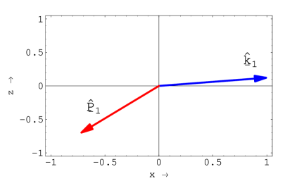
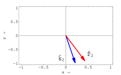
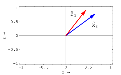
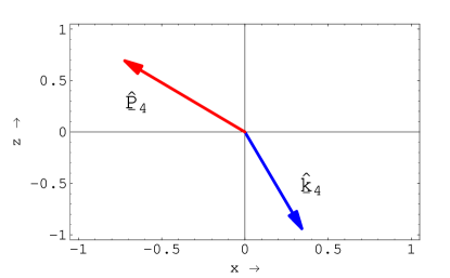
Figure 2: The orientations of the unit vectors $\hat{{\underline{k}}}_{j}={\underline{k}}_{j}/k_{j}$ and $\hat{{\underline{P}}}_{j}={\underline{P}}_{j}/P_{j}$ ($j\in\left[1,4\right]$) in the $xz$ plane for $\kappa=4k_{0}$, $\epsilon=3$, $\epsilon_{g}=1$, $\epsilon_{z}=2.5$, $\xi=10$, $\xi_{g}=6$, $\xi_{z}=7$, $\mu=2$, $\mu_{g}=0.5$ and $\mu_{z}=1.5$.

References

- [1] T.G. Mackay, Linear and nonlinear homogenized composite mediums as metamaterials, Electromagnetics 25 (2005), 461–481.
- [2] T.G. Mackay and A. Lakhtakia, Electromagnetic fields in linear bianisotropic mediums, Prog Optics (2007), to appear.
- [3] A. Lakhtakia, Beltrami fields in chiral media, World Scientific, Singapore, 1994.
- [4] B. Lax and K.J. Button, Microwave ferrites and ferrimagnetics. McGraw–Hill, New York, NY, USA, 1962.
- [5] R.E. Collin, Foundations for microwave engineering, McGraw–Hill, New York, NY, USA, 1966.
- [6] W.S. Weiglhofer, A. Lakhtakia and B. Michel, On the constitutive parameters of a chiroferrite composite medium, Microwave Opt Technol Lett 18 (1998), 342–345.
- [7] W.S. Weiglhofer and T.G. Mackay, Numerical studies of the constitutive parameters of a chiroplasma composite medium, Arch Elektron Übertrag 54 (2000), 259–265.
- [8] T.G. Mackay and A. Lakhtakia, Plane waves with negative phase velocity, Phys Rev E 69 (2004), 026602.
- [9] A. Lakhtakia, V.V. Varadan and V.K. Varadan, A parametric study of microwave reflection characteristics of a planar achiral–chiral interface, IEEE Trans Electromag Compat 28 (1986), 90–95.
- [10] T.G. Mackay, Plane waves with negative phase velocity in isotropic chiral mediums, Microwave Opt Technol Lett 45 (2005), 120–121; erratum 47 (2005), 406.
- [11] A. Baev, M. Samoc, P.N. Prasad, M. Krykunov and J. Autschbach, A quantum chemical approach to the design of chiral negative index materials, Opt Exp 15 (2007), 5730–5741.
- [12] S.A. Ramakrishna, Physics of negative refractive index materials, Rep Prog Phys 68 (2005), 449–521.
- [13] C. Zhang and T.J. Cui, Negative reflections of electromagnetic waves in chiral media, arXiv:physics/0610172.
- [14] M. Faryad and Q.A. Naqvi, Cylindrical reflector in chiral medium supporting simultaneously positive phase velocity and negative phase velocity, J Electromag Waves Applics 22 (2008), 563–572.
- [15] Y.Wang, X. Zha, and J. Yan, Reflection and refraction of light at the interface of a uniaxial bicrystal, Europhys Lett 72 (2005), 830–836.
- [16] N. Engheta, D.L. Jaggard and M.W. Kowarz, Electromagnetic waves in Faraday chiral media, IEEE Trans Antennas Propagat 40 (1992), 367–374.
- [17] W.S. Weiglhofer and A. Lakhtakia, The correct constitutive relations of chiroplasmas and chiroferrites, Microwave Opt Technol Lett 17 (1998), 405–408.
- [18] J. Gerardin and A. Lakhtakia, Conditions for Voigt wave propagation in linear, homogeneous, dielectric mediums, Optik 112 (2001), 493–495.