Nonlinear Dynamics of the Parker Scenario for Coronal Heating

Abstract

The Parker or field line tangling model of coronal heating is studied comprehensively via long-time high-resolution simulations of the dynamics of a coronal loop in cartesian geometry within the framework of reduced magnetohydrodynamics (RMHD). Slow photospheric motions induce a Poynting flux which saturates by driving an anisotropic turbulent cascade dominated by magnetic energy. In physical space this corresponds to a magnetic topology where magnetic field lines are barely entangled, nevertheless current sheets (corresponding to the original tangential discontinuities hypothesized by Parker) are continuously formed and dissipated.

Current sheets are the result of the nonlinear cascade that transfers energy from the scale of convective motions ($\sim 1,000\,km$) down to the dissipative scales, where it is finally converted to heat and/or particle acceleration. Current sheets constitute the dissipative structure of the system, and the associated magnetic reconnection gives rise to impulsive “bursty” heating events at the small scales. This picture is consistent with the slender loops observed by state-of-the-art (E)UV and X-ray imagers which, although apparently quiescent, shine bright in these wavelengths with little evidence of entangled features.

The different regimes of weak and strong MHD turbulence that develop, and their influence on coronal heating scalings, are shown to depend on the loop parameters, and this dependence is quantitatively characterized: weak turbulence regimes and steeper spectra occur in stronger loop fields and lead to larger heating rates than in weak field regions.

1. INTRODUCTION

In a previous letter (Rappazzo et al., 2007) we described simulations, within the framework of RMHD in cartesian geometry, aimed at solving the Parker field-line tangling (coronal heating) problem (Parker, 1972, 1988). We also developed a phenomenological model for nonlinear interactions, taking into account the inertial photospheric line-tying effect, which explained how the average coronal heating rate would depend on the only free parameter present in the simulations, namely the ratio of the coronal loop Alfvén crossing time and the photospheric eddy turnover time. This paper is devoted to a more detailed discussion of the numerical simulations and of the relationship between this work, the original Parker conjecture, and the nanoflare scenario of coronal heating.

Parker’s book (Parker, 1994) is devoted to an examination of the basic theorem of magnetostatics, namely that the lowest available energy state of a magnetic field in an infinitely conducting fluid contains surfaces of tangential discontinuity, or current sheets. It is Parker’s conjecture that the continuous footpoint displacement of coronal magnetic field lines must lead to the development of such discontinuities as the field continuously tries to relax to its equilibrium state, and it is the dynamical interplay of energy accumulation via footpoint motion and the bursty dissipation in the forming current sheets which gives rise to the phenomenon of the high temperature solar corona, heated by the individual bursts of reconnection, or nanoflares.

What then does turbulence have to do with the nanoflare heating scenario? Parker himself strongly criticizes the use of the “t” word, the formation of the current sheets being due in his opinion to the “requirement for ultimate static balance of the Maxwell stresses”. But what better way is there to describe the nonlinear global dynamics of a magnetically dominated plasma in which the formation of an equilibrium state containing current sheets is the inevitable asymptotic state (once the photospheric driver is turned off)?

The striving of the global magnetic field toward a state containing current sheets must occur through local violations of the force-free condition, the induction of local flows, the collapse of the currents into ever thinner layers: a nonlinear process generating ever smaller scales. From the spectral point of view, a power law distribution of energy as a function of scale is expected, even though the kinetic energy is much smaller than the magnetic energy. The last two statements are clear indications that the word turbulence provides a correct description of the dynamical process.

A final important issue is whether the overall dissipated power tends to a finite value as the resistivity and viscosity of the coronal plasma become arbitrarily small. That this must be the case is easy to understand (see § 3.3). For suppose that for an arbitrary, continuous, foot-point displacement the coronal field were only to map the foot-point motion, and that there were no non-linear interactions, i.e. the Lorentz force and convective derivatives were negligible everywhere. In this case, the magnetic field and the currents in the corona would then grow linearly in time, until the coronal dissipation at the scale of photospheric motions balanced the forcing. The amplitudes of the coronal fields and currents would then be inversely proportional to resistivity (eqs. (30)-(31)), and the dissipated power, product of resistivity and square of the current, would also scale as the inverse power of the resistivity (eq. (33)). In other words, the smaller the resistivity in the corona, the higher the power dissipated would be. But the amplitudes can not become arbitrarily large, because non-linear effects intervene to stop the increase in field amplitudes, increasing the effective dissipation at a given resistivity. Since the power can not continue to increase monotonically as the resistivity is decreased, it is clear that at some point non-linear interactions must limit the dissipated power to a finite value, regardless of the value of the resistivity. Finite dissipation at arbitrarily small values of dissipative coefficients is another definition of a turbulent system.

All this assuming that a statistically stationary state may be reached in a finite time, a question closely related to the presence of finite time singularities in 3D magnetohydrodynamics. It now appears that magnetic field relaxation in an unforced situation does not lead to the development of infinitely thin current sheets in a finite time, but rather the current development appears to be only exponential in time (Grauer and Marliani, 2000). In forced numerical simulations, as the ones we will describe in detail here, this is a moot point: for all intents and purposes a statistically stationary state is achieved at a finite time independent of resistivity for sufficiently high resolution. In fact, even if the growth is exponential, we can estimate that the width of the current sheets reaches the meter-scale in a few tens Alfvén crossing times $\tau_{\mathcal{A}}$. A typical value is $\tau_{\mathcal{A}}=40\,s$, so that this initial time is not only finite, but also short compared with an active region timescale. Once the steady state has been reached this phenomenon is no longer important. The nonlinear regime is in fact characterized by the presence of numerous current sheets, so that while some of them are being dissipated others are being formed, and a statistical steady state is maintained.

It therefore seems that the Parker field-line tangling scenario of coronal heating may be described as a particular instance of magnetically dominated MHD turbulence. Numerous analytical and numerical models of this process have been presented in the past, each discussing in some detail aspects of the general problem as presented above (Parker, 1972, 1988; Heyvaerts &Priest, 1992; van Ballegooijen, 1986; Berger, 1991; Sturrock and Uchida, 1981; Gomez & Ferro-Fontan, 1992; Mikic et al., 1989; Hendrix & Van Hoven, 1996; Longcope & Sudan, 1994; Dmitruk & Gómez, 1999; Einaudi et al., 1996; Georgoulis et al., 1998; Dmitruk et al., 1998; Einaudi & Velli, 1999).

The numerical simulations presented here bring closure to the original question as posed in cartesian geometry by Parker, starting from a uniform axial magnetic field straddling from one boundary plane to another, subject to continuous independent footpoint motions in either photosphere. This does not imply that we have fully solved the coronal heating problem as due to footpoint dragging by the photospheric velocity field.

A number of relevant effects have been neglected: first, the field line expansion between the photosphere and corona, which, if the photospheric flux is confined to bundles in granular and supergranular network lanes, would allow the mapping of the photospheric velocity field to the coronal volume to contain discontinuities. We are presently carrying out a dedicated set of simulations to capture this effect. Second, the projection of the 3D photospheric velocity to 2D coronal base motions parallel to the photosphere also introduces compressibility in the forcing flow, again neglected here. Third, we have considered stationary photospheric flows. The effect of a finite eddy-turnover time in the flow was considered in Einaudi et al. (1996); Georgoulis et al. (1998) in 2 dimensions, and in the “3 dimensional” shell model calculations of Buchlin & Velli (2007). These showed that time-dependence does not change things substantially provided the flow pattern does not contain degenerate symmetries, a fact confirmed by shorter simulations we defer to a future paper. Finally, we do not address the more realistic case of a single photosphere with curved coronal loops, such as the simulations presented recently by Gudiksen & Nordlund (2005). While this approach has advantages when investigating the coronal loop dynamics within its coronal neighborhood, modeling a larger part of the solar corona numerically drastically reduces the number of points occupied by the coronal loops. At the moment the very low resolution attainable with this kind of simulations does not allow the development of turbulence with a well-developed inertial range. The transfer of energy from the scale of convection cells $\sim 1000\,km$ toward smaller scales is inhibited, because the smaller scales are not resolved (their linear resolution is $\sim 500\,km$). Thus, these simulations have not been able to shed light on the detailed coronal statistical response nor on the different regimes which may develop and how they depend on the coronal magnetic field crossing time and the photospheric eddy turnover time.

In § 2 we introduce the coronal loop model, whose properties are qualitatively analyzed in § 3. The results of our simulations are described in § 4, and their turbulence properties are analyze in more detail in § 5. Finally in § 6 we summarize and discuss our results.

2. PHYSICAL MODEL

A coronal loop is a closed magnetic structure threaded by a strong axial field, with the footpoints rooted in the photosphere. This makes it a strongly anisotropic system, as measured by the relative magnitude of the Alfvén velocity associated with the axial magnetic field $v_{\mathcal{A}}\sim 2000\ \textrm{km}\,\textrm{s}^{-1}$ compared to the typical photospheric velocity $u_{ph}\sim 1\ \textrm{km}\,\textrm{s}^{-1}$.

We study the loop dynamics in a simplified Cartesian geometry, neglecting field line curvature, i.e. the toroidality of loops. Our loop is a “straightened out” box, with an orthogonal square cross section of size $\ell$ (along which the x-y directions lie), and an axial length $L$ (along the z direction) embedded in an axial homogeneous uniform magnetic field $\mathbf{B}_{0}=B_{0}\ \mathbf{e}_{z}$. This simplified geometry allows us to perform simulations with both high numerical resolution and long-time duration.

In § 2.1 we introduce the equations used to model the dynamics, while in § 2.2 we give the boundary and initial conditions used in our numerical simulations.

2.1. Governing Equations

The dynamics of a plasma embedded in a strong axial magnetic field are well described by the equations of reduced MHD (RMHD) (Kadomtsev & Pogutse, 1974; Strauss, 1976; Montgomery, 1982).

These equations are valid for a plasma with small ratio of kinetic to magnetic pressures, in the limit of a large loop-aspect ratio ($\epsilon=l/L\ll 1$, $L$ being the length of the loop and $l$ being the minor radius of the loop) and of a small ratio of poloidal to axial magnetic field ($b_{\perp}/B_{0}\leq\epsilon$). In dimensionless form they can be written as:

$$\frac{\partial\boldsymbol{u}_{\perp}}{\partial t}+\left(\boldsymbol{u}_{\perp}\cdot\boldsymbol{\nabla}_{\perp}\right)\boldsymbol{u}_{\perp}=-\boldsymbol{\nabla}_{\perp}\left(p+\frac{\boldsymbol{b}_{\perp}^{2}}{2}\right)\\ +\left(\boldsymbol{b}_{\perp}\cdot\boldsymbol{\nabla}_{\perp}\right)\boldsymbol{b_{\perp}}+c_{\mathcal{A}}\,\frac{\partial\boldsymbol{b}_{\perp}}{\partial z}+\frac{(-1)^{n+1}}{Re_{n}}\boldsymbol{\nabla}^{2n}_{\perp}\boldsymbol{u}_{\perp},$$ (1)

$$\frac{\partial\boldsymbol{b}_{\perp}}{\partial t}=\left(\boldsymbol{b}_{\perp}\cdot\boldsymbol{\nabla}_{\perp}\right)\boldsymbol{u_{\perp}}-\left(\boldsymbol{u}_{\perp}\cdot\boldsymbol{\nabla}_{\perp}\right)\boldsymbol{b_{\perp}}\\ +c_{\mathcal{A}}\,\frac{\partial\boldsymbol{u}_{\perp}}{\partial z}+\frac{(-1)^{n+1}}{Re_{n}}\boldsymbol{\nabla}^{2n}_{\perp}\boldsymbol{b}_{\perp},$$ (2)

$$\boldsymbol{\nabla}_{\perp}\cdot\boldsymbol{u}_{\perp}=0,\qquad\boldsymbol{\nabla}_{\perp}\cdot\boldsymbol{b}_{\perp}=0,\qquad\qquad\qquad\quad$$ (3)

where $\mathbf{u}_{\perp}$ and $\mathbf{b}_{\perp}$ are the components of the velocity and magnetic fields perpendicular to the mean field, and $p$ is the kinetic pressure. The gradient operator likewise has only components in the $x$-$y$ plane perpendicular to the axial direction $z$, i.e.

$$\mathbf{\nabla}_{\perp}=\mathbf{e}_{x}\,\frac{\partial}{\partial x}+\mathbf{e}_{y}\,\frac{\partial}{\partial y},$$ (4)

while the dynamics in the planes is coupled to the axial direction through the linear terms $\propto\partial_{z}$.

To render the equation non dimensional magnetic fields have first been expressed in velocity units by dividing by $\sqrt{4\pi\rho_{0}}$ (where $\rho_{0}$ is a density supposed homogeneous and constant), i.e. considering the associated Alfvén velocities ($b\rightarrow b/\sqrt{4\pi\rho_{0}}$), and then both velocity and magnetic fields have been normalized to a typical photospheric velocity $u_{ph}$; lengths and times have been expressed in units of the perpendicular length of the computational box $\ell$ and its related “eddy turnover time” $t_{\perp}=\ell/u_{ph}$.

As a result, in equations (1)-(2), the linear terms $\propto\partial_{z}$ are multiplied by the dimensionless Alfvén velocity $c_{\mathcal{A}}=v_{\mathcal{A}}/u_{ph}$, i.e the ratio between the Alfvén velocity associated with the axial magnetic field $v_{\mathcal{A}}=B_{0}/\sqrt{4\pi\rho_{0}}$, and the photospheric velocity $u_{ph}$.

The index $n$ is called dissipativity: the diffusive terms adopted in equations (1)-(2) correspond to ordinary diffusion for $n=1$ and to so-called hyperdiffusion for $n>1$. When $n=1$ the $\mathbf{\nabla}_{\perp}^{2}/Re$ diffusive operator is recovered, so that $Re_{1}=Re=Re_{m}$ corresponds to the kinetic and magnetic Reynolds number (considered of equal and uniform value):

$$Re=\frac{\rho_{0}\,\ell u_{ph}}{\nu},\qquad Re_{m}=\frac{4\pi\rho_{0}\,\ell u_{ph}}{\eta c^{2}},$$ (5)

where viscosity $\nu$ and resistivity $\eta$ are taken to be constant and uniform ($c$ is the speed of light).

We have performed numerical simulations with both $n=1$ and $n=4$. Hyperdiffusion is used because with a limited resolution the diffusive timescales associated with ordinary diffusion are small enough to affect the large scale dynamics and render very difficult the resolution of an inertial range, even with a grid with 512x512 points in the x-y plane (the highest resolution grid we used for the plane). The diffusive time $\tau_{n}$ at the scale $\lambda$ associated with the dissipative terms used in (1)-(2) is given by:

$$\tau_{n}\sim Re_{n}\,\lambda^{2n}$$ (6)

While for $n=1$ the diffusive time decreases relatively slowly towards smaller scales, for $n=4$ it decreases far more rapidly. This allows to have longer diffusive timescales at large spatial scales and similar diffusive timescales at the resolution scale. Numerically we require that the diffusion time at the resolution scale $\lambda_{min}=1/N$, where N is the number of grid points, to be of the same order of magnitude for both normal and hyperdiffusion, i.e.

$$\frac{Re_{1}}{N^{2}}\sim\frac{Re_{n}}{N^{2n}}\quad\longrightarrow\quad Re_{n}\sim Re_{1}\,N^{2(n-1)}$$ (7)

For instance a numerical grid with $N=512$ points which requires a Reynolds number $Re_{1}=800$ with ordinary diffusion, can implement $Re_{4}\sim 10^{19}$, removing diffusive effects at the large scales, and allowing (if present) the resolution of an inertial range.

The numerical integration of the RMHD equations (1)-(3) is substantially simplified by using the potentials of the velocity ($\varphi$) and magnetic field ($\psi$),

$$\mathbf{u}_{\perp}=\mathbf{\nabla}\times\left(\varphi\,\mathbf{e}_{z}\right),\qquad\mathbf{b}_{\perp}=\mathbf{\nabla}\times\left(\psi\,\mathbf{e}_{z}\right),$$ (8)

linked to vorticity and current by $\omega=-\mathbf{\nabla}^{2}_{\perp}\varphi$ and $j=-\mathbf{\nabla}^{2}_{\perp}\psi$.

We solve numerically equations (1)-(3) written in terms of the potentials (see Rappazzo et al. (2007)) in Fourier space, i.e. we advance the Fourier components in the $x$-$y$ directions of the scalar potentials $\varphi$ and $\psi$. Along the $z$ direction no Fourier transform is performed so that we can impose non-periodic boundary conditions (specified in § 2.2), and a central second-order finite difference scheme is used. In the $x$-$y$ plane a Fourier pseudospectral method is implemented. Time is discretized with a third-order Runge-Kutta method.

We use a computational box with an aspect ratio of 10, which spans

$$0\leq x,y\leq 1,\qquad 0\leq z\leq 10.$$ (9)

2.2. Boundary and Initial Conditions

As boundary conditions at the photospheric surfaces ($z=0,\ L$) we impose two independent velocity patterns, intended to mimic photospheric motions, made up of large spatial scale projected convection cell flow patterns constant in time. The velocity potential at each boundary is given by:

$$\varphi(x,y)=\frac{1}{\sqrt{\sum_{mn}\alpha_{mn}^{2}}}\ \sum_{k,l}\frac{\ell\,\alpha_{kl}}{2\pi\sqrt{k^{2}+l^{2}}}\ \\ \sin\left[\frac{2\pi}{\ell}\left(kx+ly\right)+2\pi\,\xi_{kl}\right]$$ (10)

We excite all the wave number values $(k,l)\in\mathbb{Z}^{2}$ included in the range $3\leq\left(k^{2}+l^{2}\right)^{1/2}\leq 4$, so that the resulting average injection wavenumber is $k_{c}\sim 3.4$, and the average injection scale $\ell_{c}$, the convection cell scale, is given by $\ell_{c}=\ell/k_{c}$. $\alpha_{kl}$ and $\xi_{kl}$ are two sets of random numbers whose values range between $0$ and $1$, and are independently chosen for the two boundary surfaces. The normalization adopted in eq. (10) sets the value of the corresponding velocity rms (see eq. (8)) to $1/\sqrt{2}$, i.e.

$$\int_{0}^{\ell}\!\!\!\int_{0}^{\ell}\mathrm{d}x\,\mathrm{d}y\ \left(u_{x}^{2}+u_{y}^{2}\right)=\frac{1}{2}$$ (11)

At time $t=0$ no perturbation is imposed inside the computational box, i.e. $\mathbf{b}_{\perp}=\mathbf{u}_{\perp}=0$, and only the axial magnetic field $B_{0}$ is present: the subsequent dynamics are then the effect of the photospheric forcing (10) on the system, as described in the following sections.

3. ANALYSIS

In order to clarify aspects of the linear and nonlinear properties of the RMHD system, we provide an equivalent form of the equations (1)-(3). In terms of the Elsässer variables $\mathbf{z}^{\pm}=\mathbf{u}_{\perp}\pm\mathbf{b}_{\perp}$, which bring out the basic symmetry of the equations in terms of parallel and anti-parallel propagating Alfvén waves, they can be written as

$$\frac{\partial\boldsymbol{z}^{+}}{\partial t}=-\left(\boldsymbol{z}^{-}\cdot\boldsymbol{\nabla}_{\perp}\right)\boldsymbol{z}^{+}+c_{\mathcal{A}}\,\frac{\partial\boldsymbol{z}^{+}}{\partial z}\\ +\frac{(-1)^{n+1}}{Re_{n}}\boldsymbol{\nabla}^{2n}_{\perp}\boldsymbol{z}^{+}-\boldsymbol{\nabla}_{\perp}P,$$ (12)

$$\frac{\partial\boldsymbol{z}^{-}}{\partial t}=-\left(\boldsymbol{z}^{+}\cdot\boldsymbol{\nabla}_{\perp}\right)\boldsymbol{z}^{-}-c_{\mathcal{A}}\,\frac{\partial\boldsymbol{z}^{-}}{\partial z}\\ +\frac{(-1)^{n+1}}{Re_{n}}\boldsymbol{\nabla}^{2n}_{\perp}\boldsymbol{z}^{-}-\boldsymbol{\nabla}_{\perp}P,$$ (13)

$$\boldsymbol{\nabla}_{\perp}\cdot\boldsymbol{z}^{\pm}=0,\qquad\qquad\qquad\qquad\qquad\qquad\qquad\ \ \,$$ (14)

where $P=p+\mathbf{b}_{\perp}^{2}/2$ is the total pressure, and is linked to the nonlinear terms by incompressibility (14):

$$\mathbf{\nabla}_{\perp}^{2}P=-\sum_{i,j=1}^{2}\Big{(}\partial_{i}z_{j}^{-}\Big{)}\Big{(}\partial_{j}z_{i}^{+}\Big{)}.$$ (15)

In terms of the Elsässer variables $\mathbf{z}^{\pm}=\mathbf{u}_{\perp}\pm\mathbf{b}_{\perp}$, a velocity pattern $\mathbf{u}_{\perp}^{0,L}$ at upper or lower boundary surface becomes the constraint $\mathbf{z}^{+}+\mathbf{z}^{-}=2\mathbf{u}_{\perp}^{0,L}$ at that boundary. Since, in terms of characteristics (which in this case are simply $\mathbf{z}^{\pm}$ themselves), we can specify only the incoming wave (while the outgoing wave is determined by the dynamics inside the computational box), this velocity pattern implies a reflecting condition at the top ($z=L$) and bottom ($z=0$) planes:

$$\mathbf{z^{-}}=-\mathbf{z^{+}}+2\,\mathbf{u}^{0}_{\perp}\quad\textrm{at}\ z=0,$$ (16)

$$\mathbf{z^{+}}=-\mathbf{z^{-}}+2\,\mathbf{u}^{L}_{\perp}\quad\textrm{at}\ z=L.$$ (17)

The linear terms ($\propto\partial_{z}$) in equations (12)-(13) give rise to two distinct wave equations for the $\mathbf{z}^{\pm}$ fields, which describe Alfvén waves propagating along the axial direction $z$. This wave propagation, which is present during both the linear and nonlinear regimes, is responsible for the continuous energy influx on large perpendicular scales (see eq. (10)) from the boundaries into the loop. The nonlinear terms $\left(\mathbf{z}^{\mp}\cdot\mathbf{\nabla}_{\perp}\right)\mathbf{z}^{\pm}$ are then responsible for the transport of this energy from the large scales toward the small scales, where energy is finally dissipated, i.e. converted to heat and/or particle acceleration.

A well-known important feature of the nonlinear terms in equations (12)-(14) is the absence of self-coupling, i.e.  only counterpropagating waves interact non-linearly, and if one of the two fields $\mathbf{z}^{\pm}$ is zero, there are no nonlinear interactions at all. This fact, i.e.  that counter-propagating wave-packets may interact only while they are crossing each other, lies at the basis of the so-called Alfvén effect (Iroshnikov, 1964; Kraichnan, 1965), which ultimately renders the nonlinear timescales longer and slows down the dynamics.

From this description three different timescales arise naturally: $\tau_{\mathcal{A}}$, $\tau_{ph}$ and $\tau_{nl}$. $\tau_{\mathcal{A}}=L/v_{\mathcal{A}}$ is the crossing time of the Alfvén waves along the axial direction $z$, i.e. the time it takes for an Alfvén wave to cover the loop length $L$. $\tau_{ph}\sim 5~{}m$ is the characteristic time associated with photospheric motions, while $\tau_{nl}$ is the nonlinear timescale.

For a typical coronal loop $\tau_{\mathcal{A}}\ll\tau_{ph}$. For instance for a coronal loop long $L=40,000~{}km$ and with an Alfvén velocity $v_{\mathcal{A}}=2,000~{}km\,s^{-1}$ we obtain $\tau_{\mathcal{A}}=20~{}s$, which is small compared to $\tau_{ph}\sim 5~{}m=300~{}s$. This is the reason we carried out simulations with a photospheric forcing constant in time (see eq. (10)), i.e. for which formally $\tau_{ph}=\infty$.

In the RMHD ordering the nonlinear timescale $\tau_{nl}$ is bigger than the Alfvén crossing time $\tau_{\mathcal{A}}$. As we shall see this ordering is maintained during our simulations and we will give analytical estimates of the value of $\tau_{nl}$ as a function of the characteristic parameters of the system.

An important feature of equations (12)-(14) that we will use to generalize our results is that, apart from the Reynolds numbers, there is only one fundamental non-dimensional parameter:

$$f=\frac{\ell_{c}\,v_{\mathcal{A}}}{L\,u_{ph}}.$$ (18)

Hence all the physical quantities which result from the dynamical evolution, e.g. energy, Poynting flux, heating rate, timescales, etc., must depend on this single parameter $f$.

3.1. Energy Equation

From equations (1)-(3), with $n=1$, and considering the Reynolds numbers equal, the following energy equation can be derived:

$$\frac{\partial}{\partial t}\left(\frac{1}{2}\mathbf{u}_{\perp}^{2}+\frac{1}{2}\mathbf{b}_{\perp}^{2}\right)=-\mathbf{\nabla}\cdot\mathbf{S}-\frac{1}{Re}\left(\mathbf{j}^{2}+\mathbf{\omega}^{2}\right),$$ (19)

where $\mathbf{S}=\mathbf{B}\times(\mathbf{u}\times\mathbf{B})$ is the Poynting vector. As expected the energy balance of the system described by eq. (19) is due to the competition between the energy (Poynting) flux flowing into the computational box and the ohmic and viscous dissipation. Integrating eq (19) over the whole box the only relevant component of the Poynting vector is the component along the axial direction $z$, because in the $x$-$y$ plane periodic boundary conditions are used and their contribution to the Poynting flux is null. As $\mathbf{B}=c_{\mathcal{A}}\,\mathbf{e}_{z}+\mathbf{b}_{\perp}$ and $\mathbf{u}=\mathbf{u}_{\perp}$, this is given by

$$S_{z}=\mathbf{S}\cdot\mathbf{e}_{z}=-c_{\mathcal{A}}\left(\mathbf{u}_{\perp}\cdot\mathbf{b}_{\perp}\right).$$ (20)

Considering that the velocity fields at the photospheric boundaries are given by $\mathbf{u}_{\perp}^{0}$ and $\mathbf{u}_{\perp}^{L}$, for the integrated energy flux we obtain

$$S=c_{\mathcal{A}}\int_{z=L}\!\mathrm{d}a\,\left(\mathbf{u}_{\perp}^{L}\cdot\mathbf{b}_{\perp}\right)-c_{\mathcal{A}}\int_{z=0}\!\mathrm{d}a\,\left(\mathbf{u}_{\perp}^{0}\cdot\mathbf{b}_{\perp}\right).$$ (21)

The injected energy flux therefore depends not only on the photospheric forcing and the axial Alfvén velocity (which have fixed values), but also on the value of the magnetic fields at the boundaries, which is determined by the dynamics of the system inside the computational box: the injection of energy depends on the nonlinear dynamics which develops, and viceversa.

The simplified topology investigated in this paper, i.e.  a strong axial magnetic field whose footpoints are dragged by 2D orthogonal motions applies to regions where emerging flux may be neglected. Consider the axial component of the velocity $u_{z}$ field carrying new magnetic field ($\mathbf{b}_{\perp}^{ef}$) into the corona. The associated Poynting flux is

$$S_{z}^{ef}=\left(\mathbf{b}_{\perp}^{ef}\right)^{2}u_{z}.$$ (22)

This flux component is negligible when $S_{z}^{ef}<S_{z}$, i.e., since all the components of the photospheric velocity fields are of the same order, $u_{z}\sim u_{ph}$, when

$$\left(b_{\perp}^{ef}\right)^{2}<B_{0}\,b_{\perp}^{turb}.$$ (23)

In § 5.2 we give an estimate of the value of the field $b_{\perp}^{turb}$ generated by the field-line dragging, and will be able to quantify for which value of $b_{\perp}^{ef}$ the emerging flux can be neglected.

3.2. Linear Stage

For $t<\tau_{nl}$ nonlinear terms can be neglected. Neglecting also the diffusion terms, which play no role on large scales, equations (1)-(3) reduce to two simple wave equations. Coupled with the boundary conditions (10) the solution for times longer than the crossing time $\tau_{\mathcal{A}}$ reads:

$$\mathbf{b}_{\perp}(x,y,z,t)=\left[\mathbf{u}^{L}(x,y)-\mathbf{u}^{0}(x,y)\right]\ \frac{t}{\tau_{\mathcal{A}}},$$ (24)

$$\mathbf{u}_{\perp}(x,y,z,t)=\mathbf{u}^{L}(x,y)\frac{z}{L}+\mathbf{u}^{0}(x,y)\left(1-\frac{z}{L}\right).$$ (25)

This shows that A) the loop velocity field is bounded by the imposed photospheric fields and b) the magnetic field grows linearly in time, uniform along the loop, while mapping the photospheric velocity field in the perpendicular planes. Therefore, for a generic set of velocities $\mathbf{u}^{L}$ and $\mathbf{u}^{0}$, the resulting magnetic fields (24)-(25) give rise to non-vanishing forces in the perpendicular planes which grow quadratically in time, becoming dynamically important after a certain interval (Buchlin & Velli, 2007).

There exists a (singular) set of velocity forcing patterns, for which the generated coronal field has a vanishing Lorentz force. For simplicity consider $\mathbf{u}^{L}=0$: in terms of potentials it follows that $\psi=-\varphi^{0}\,t/\tau_{\mathcal{A}}$ and $\varphi=\varphi^{0}\,(1-z/L)$ (where $\mathbf{u}^{0}_{\perp}=\mathbf{\nabla}\times\left(\varphi^{0}\,\mathbf{e}_{z}\right)$). In this case both $\mathbf{b}_{\perp}$ and $\mathbf{u}_{\perp}$ are proportional to $\mathbf{\nabla}_{\perp}\times(\varphi^{0}\,\mathbf{e}_{z})$. The condition for the vanishing of nonlinear terms then becomes

$$\mathbf{\nabla}\left(\mathbf{\nabla}^{2}\,\varphi^{0}\right)\times\mathbf{\nabla}\varphi^{0}=0,\quad\textrm{with}\quad\varphi^{0}=\varphi^{0}\left(x,y\right).$$ (26)

This condition is then satisfied by those fields for which the laplacian is constant along the streamlines of the field. As $\omega=-\mathbf{\nabla}^{2}\,\varphi$ this is equivalent to the statement that the vorticity is constant along the streamlines. This condition is in general not verified, unless very symmetric functions are chosen, e.g. in cartesian geometry by any 1D function like $\varphi^{0}=f(x)$, and in polar coordinates by any radial function $\varphi^{0}=g(r)$.

Generally speaking even in such peculiar configurations non-linear interactions will arise due to the onset of instabilities. We defer discussion of these extreme examples to a subsequent paper, the random photospheric fields  (10) discussed here always giving rise to non-vanishing forces .

Inserting the linear evolution fields  (24) in the expression for the integrated energy flux (21), we find

$$S=c_{\mathcal{A}}\int\!\mathrm{d}a\,|\mathbf{u}^{L}-\mathbf{u}^{0}|^{2}\cdot\frac{t}{\tau_{\mathcal{A}}},$$ (27)

i.e. the Poynting flux $S$ grows linearly in time until such a time that non-linear interactions set in.

A similar linear analysis was already performed by Parker (1988), who noted that if this is the mechanism responsible for coronal heating, then the energy flux $S_{z}\sim S/\ell^{2}$ must approach the value $S_{z}\sim 10^{7}\,erg\,cm^{2}\,s^{-1}$ necessary to sustain an active region before a saturating mechanism, magnetic reconnection of singular current sheets in Parker’s language, takes over.

In fact however the value reached by $S_{z}$ depends on the nonlinear dynamics, its value self-consistently determined by solving the nonlinear problem. An $S_{z}$ too small compared with observational constraints would then rule out the Parker model.

3.3. Effects of Diffusion

The linear solution (24)-(25) has been obtained without taking into account the diffusive terms. This is justified, given the large value of the Reynolds numbers for the solar corona. But numerically it can be important. At very low resolution diffusion is so important that little or no nonlinear dynamics develop and the system reaches a balance between the photospheric forcing and diffusion of the large scale fields.

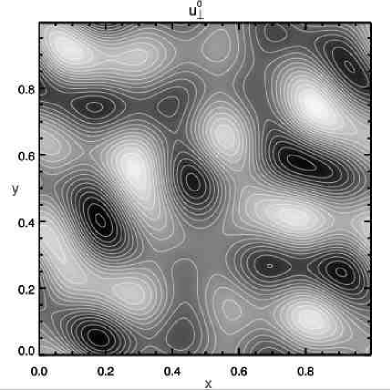
Figure 1.— Streamlines of the velocity field $\mathbf{u}_{\perp}^{0}$, the boundary forcing at the bottom plane $z=0$ for run A. In lighter vortices the velocity field is directed anti-clockwise while in darker vortices it is directed clockwise. The cross-section shown in the figure is roughly $4000\times 4000\,km^{2}$, where the typical scale of a convective cell is $1000\,km$.

One can attempt to bypass the non-linear problem by adopting a much smaller “turbulent” value of the Reynolds number (Heyvaerts &Priest, 1992). For this “ad hoc” value of the Reynolds number the average dissipation would be the same as in the high Reynolds number active turbulence limit. Linearizing equation (2) (with $n=1$ and $Re_{1}=Re$), we obtain

$$\frac{\partial\mathbf{b}_{\perp}}{\partial t}=c_{\mathcal{A}}\frac{\partial\mathbf{u}_{\perp}}{\partial z}+\frac{1}{Re}\mathbf{\nabla}^{2}_{\perp}\mathbf{b}_{\perp}.$$ (28)

Taking into account that the forcing velocities are dominated by components at the injection scale $\ell_{c}$ (see eq. (10)), the relation $\mathbf{\nabla}^{2}_{\perp}\varphi=-\left(2\pi/\ell_{c}\right)^{2}\varphi$, where $\ell_{c}=\ell/k_{c}$ with the average wavenumber $k_{c}\sim 3.4$, is approximately valid. Integrating then eq. (28) over $z$ and dividing by the length $L$, we obtain for $\mathbf{b}_{\perp}$ averaged along $z$:

$$\frac{\partial\mathbf{b}_{\perp}}{\partial t}=\frac{c_{\mathcal{A}}}{L}\left[\mathbf{u}^{L}\left(x,y\right)-\mathbf{u}^{0}\left(x,y\right)\right]-\frac{\left(2\pi\right)^{2}}{\ell_{c}^{2}Re}\mathbf{b}_{\perp}.$$ (29)

Indicating with $\mathbf{u}_{ph}=\mathbf{u}^{L}-\mathbf{u}^{0}$, with $\tau_{\mathcal{R}}={\ell_{c}^{2}Re}/\left(2\pi\right)^{2}$ the diffusive time-scale and with $\tau_{\mathcal{A}}=L/c_{\mathcal{A}}$ the Alfvén crossing time, the solution is given by:

$$\boldsymbol{b}_{\perp}\left(x,y,t\right)=\boldsymbol{u}_{ph}\left(x,y\right)\frac{\tau_{\mathcal{R}}}{\tau_{\mathcal{A}}}\left[1-\exp\left(-\frac{t}{\tau_{\mathcal{R}}}\right)\right],$$ (30)

$$\left|j\left(x,y,t\right)\right|=\left|\boldsymbol{u}_{ph}\left(x,y\right)\right|\left(\frac{2\pi}{\ell_{c}}\right)\frac{\tau_{\mathcal{R}}}{\tau_{\mathcal{A}}}\times\\ \times\left[1-\exp\left(-\frac{t}{\tau_{\mathcal{R}}}\right)\right].$$ (31)

So that the magnetic energy $E_{M}$

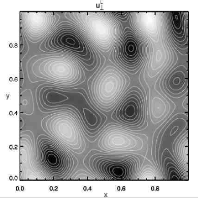
Figure 2.— Streamlines of the velocity field $\mathbf{u}_{\perp}^{L}$, the boundary forcing at the top plane $z=L$ for run A. The numerical grid has 512x512 points in the x-y planes, with a linear resolution of $\sim 8\,km$.

and the ohmic dissipation rate $J$ are given by

$$E_{M}=\frac{1}{2}\int_{V}\mathrm{d}^{3}\boldsymbol{x}\ \boldsymbol{b}_{\perp}^{2}=\\ =\frac{1}{2}\ell^{2}\,L\,u^{2}_{ph}\,\left(\frac{\tau_{\mathcal{R}}}{\tau_{\mathcal{A}}}\right)^{2}\left[1-\exp\left(-\frac{t}{\tau_{\mathcal{R}}}\right)\right]^{2},$$ (32)

$$J=\frac{1}{Re}\int_{V}\mathrm{d}^{3}\boldsymbol{x}\ j^{2}=\\ =\ell^{2}\,L\,u^{2}_{ph}\,\frac{\tau_{\mathcal{R}}}{\tau_{\mathcal{A}}^{2}}\left[1-\exp\left(-\frac{t}{\tau_{\mathcal{R}}}\right)\right]^{2},$$ (33)

where $u_{ph}$ is the rms of $\mathbf{u}_{ph}$, and with the rms of the boundary velocities $\mathbf{u}^{0}$ and $\mathbf{u}^{L}$ fixed to $1/2$ (11) we have $u_{ph}\sim 1$. Both total magnetic energy (32) and ohmic dissipation (33) grow quadratically in time for time smaller than the resistive time $\tau_{\mathcal{R}}$, while on the diffusive time scale they saturate to the values

$$E_{M}^{sat}=\frac{\ell^{6}\,c_{\mathcal{A}}^{2}\,u^{2}_{ph}\,Re^{2}}{L\,\left(2\pi k_{c}\right)^{4}},\qquad J^{sat}=\frac{\ell^{4}\,c_{\mathcal{A}}^{2}\,u^{2}_{ph}\,Re}{L\,\left(2\pi k_{c}\right)^{2}},$$ (34)

written explicitly in terms of the loop parameters and Reynolds number.

Magnetic energy saturates to a value proportional to the square of both the Reynolds number and the Alfvén velocity, while the heating rate saturates to a value that is proportional to the Reynolds number and the square of the axial Alfvén velocity. We have also used equations (32)-(33) as a check in our numerical simulations, and during the linear stage, before nonlinearity sets in they are well satisfied.

From equation (32)-(33) we can estimate the saturation time as the time at which the functions (32)-(33) reach 2/3 of the saturation values. It is approximately given by

$$\tau^{sat}\sim 2\,\tau_{\mathcal{R}}=\frac{2\,\ell^{2}Re}{\left(2\pi k_{c}\right)^{2}}$$ (35)

In the next section we describe the results of our simulations, which investigate the linear and nonlinear dynamics. The average values may be used in conjunction with 34 to define the equivalent turbulence Reynolds number.

4. NUMERICAL SIMULATIONS

Run	$c_{\mathcal{A}}$	$n_{x}\times n_{y}\times n_{z}$	n	$Re$, $Re_{4}$	$t_{max}/\tau_{\mathcal{A}}$
A	200	$512\times 512\times 200$	1	$8\cdot 10^{2}$	548
B	200	$256\times 256\times 100$	1	$4\cdot 10^{2}$	1061
C	200	$128\times 128\times 100$	1	$2\cdot 10^{2}$	2172
D	200	$128\times 128\times 100$	1	$1\cdot 10^{2}$	658
E	200	$128\times 128\times 100$	1	$1\cdot 10^{1}$	1272
F	50	$512\times 512\times 200$	4	$3\cdot 10^{20}$	196
G	200	$512\times 512\times 200$	4	$10^{19}$	453
H	400	$512\times 512\times 200$	4	$10^{20}$	77
I	1000	$512\times 512\times 200$	4	$10^{19}$	502

Table 1Summary of the simulations. $c_{\mathcal{A}}$ is the axial Alfvén velocity and $n_{x}\times n_{y}\times n_{z}$ is number of points for the numerical grid. n is the dissipativity, $n=1$ indicates normal diffusion, $n=4$ hyperdiffusion. $Re$ ($=Re_{1}$) or $Re_{4}$ indicates respectively the value of the Reynolds number or of the hyperdiffusion coefficient (see eq.(12)-(13)). The duration of the simulation $t_{max}/\tau_{\mathcal{A}}$ is given in Alfvén crossing time unit $\tau_{\mathcal{A}}=L/v_{\mathcal{A}}$.

In this section we present a series of numerical simulations, summarized in Table 1, modeling a coronal layer driven by a forcing velocity pattern constant in time. On the bottom and top planes we impose two independent velocity forcings as described in § 2.2, which result from the linear combination of large-scale eddies with random amplitudes, normalized so that the rms of the photospheric velocity is $u_{ph}\sim 1\,km\,s^{-1}$. For each simulation a different set of random amplitudes is chosen, corresponding to different patterns of the forcing velocities. A realization of this forcing with a specific choice (run A) of the random amplitudes is shown in Figures 1-2.

The length of a coronal section is taken as the unitary length. As we excite all the wavenumbers between 3 and 4, and the typical convection cell scale is $\sim 1,000\,km$, this implies that each side of our section is roughly $4,000\,km$ long. Our typical grid for the cross-sections has 512x512 grid points, corresponding to $\sim 128^{2}$ points per convective cell, and hence a linear resolution of $\sim 8~{}km$.

Between the top and bottom plates a uniform magnetic field $\mathbf{B}=B_{0}\,\mathbf{e}_{z}$ is present. The subsequent evolution is due to the shuffling of the footpoints of the magnetic field lines by the photospheric forcing.

In the different numerical simulations, keeping fixed the cross-section length ($\sim 4,000\,km$) and axial length ($\sim 40,000\,km$), we explore the behavior of the system for different values of $c_{\mathcal{A}}$, i.e. the ratio between the Alfvén velocity associated with the axial magnetic field and the rms of the photospheric motions (density is supposed uniform and constant).

Nevertheless, as shown in (18) the fundamental parameter is $f=\ell_{c}v_{\mathcal{A}}/Lu_{ph}$, so that changing $c_{\mathcal{A}}=v_{\mathcal{A}}/u_{ph}$ is equivalent to explore the behaviour of the system for different values of $f$, where the same value of $f$ can be realized with a different choice of the quantities, provided that the RMHD approximation is valid, i.e. we are describing a slender loop threaded by a strong magnetic field.

We also perform simulations with different numerical resolutions, i.e. different Reynolds numbers, and both normal ($n=1$) and hyper-diffusion ($n=4$).

The qualitative behaviour of the system is the same for all the simulations performed. In the next section we describe these qualitative features in detail for run A, and then describe the quantitative differences found in the other simulations.

4.1. Run A

In this section we present the results of a simulation performed with a numerical grid with 512x512x200 points, normal ($n=1$) diffusion with a Reynolds number $Re=800$, and the Alfvén velocity $v_{\mathcal{A}}=200\,km\,s^{-1}$ corresponding to a ratio $c_{\mathcal{A}}=v_{\mathcal{A}}/u_{ph}=200$. The streamlines of the forcing velocities applied in the top ($z=L$) and bottom ($z=0$) planes are shown in Figures 1-2. The total duration is roughly 550 axial Alfvén crossing times ($\tau_{\mathcal{A}}=L/v_{\mathcal{A}}$).

Plots of the total magnetic and kinetic energies

$$E_{M}=\frac{1}{2}\int\!\mathrm{d}V\,\mathbf{b}_{\perp}^{2},\qquad E_{K}=\frac{1}{2}\int\!\mathrm{d}V\,\mathbf{u}_{\perp}^{2},$$ (36)

and of the total ohmic and viscous dissipation rates

$$J=\frac{1}{Re}\int\!\mathrm{d}V\,\mathbf{j}^{2},\qquad\Omega=\frac{1}{Re}\int\!\mathrm{d}V\,\mathbf{\omega}^{2},$$ (37)

along with the incoming energy rate (integrated Poynting flux) $S$ (see eq. (21)), are shown in Figures 3-4. At the beginning the system has a linear behavior (see eqs. (24)-(25), and (27)), characterized by a linear growth in time for the magnetic energy, the Poynting flux and the electric current, which implies a quadratic growth for the ohmic dissipation $\propto(t/\tau_{\mathcal{A}})^{2}$, until time $t\sim 6\,\tau_{\mathcal{A}}$, when nonlinearity sets in. We can identify this time as the nonlinear timescale, i.e. $\tau_{nl}\sim 6\,\tau_{\mathcal{A}}$. The timescales of the system will be analyzed in more details in §5.5.

After this time, in the fully nonlinear stage, a statistically steady state is reached, in which the Poynting flux, i.e. the energy that is entering the system for unitary time, balances on time average the total dissipation rate ($J+\Omega$). As a result there is no average accumulation of energy in the box, beyond what has been accumulated during the linear stage, while a detailed examination of the dissipation time series (see inset in Figure 4) shows that the Poynting flux and total dissipations are decorrelated around dissipation peaks.

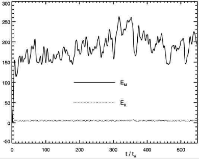
Figure 3.— Run A: High-resolution simulation with $v_{\mathcal{A}}/u_{ph}=200$, 512x512x200 grid points and $Re=800$. Magnetic ($E_{M}$) and kinetic ($E_{K}$) energies as a function of time ($\tau_{\mathcal{A}}=L/v_{\mathcal{A}}$ is the axial Alfvén crossing time).

In the diffusive case from eqs. (32)-(35), with the values of this simulation we would obtain $\tau^{sat}\sim 50\,\tau_{\mathcal{A}}$, $E_{M}^{sat}\sim 6100$ and $J^{sat}\sim 7100$; all values well beyond those of the simulation. A value of $Re=85$ would fit the simulated average dissipation, while $Re=140$ would approximately fit the average magnetic energy. In any case this would only fit the curves, but the physical phenomena would be completely different, as we describe in the following sections.

An important characteristic of the system is the magnetic predominance for both energy and dissipation (Figures 3 and 4). In the linear stage (§ 3.2) while the magnetic field grows linearly in time, the velocity field does not, and its value is roughly the sum of the boundary forcing fields. The physical interpretation is that because we are bending the axial magnetic field with a constant forcing, as a result the perpendicular magnetic field grows linearly in time, while the velocity remains limited. More formally this is a consequence of the fact that, while on the perpendicular magnetic field no boundary condition is imposed, the velocity field must approach the imposed boundary values at the photosphere both during the linear and nonlinear stages.

In Figure 5 the 2D averages in the x-y planes of the magnetic and velocity fields and of the ohmic dissipation $j^{2}/Re$, are plotted as a function of z at different times. These macroscopic quantities are smooth and present almost no structure along the axial direction. The reason is that every disturbance or gradient along the axial direction, at least considering the large perpendicular scales (for the small scales behavior see § 5 ), is smoothed out by the fast propagation of Alfvén waves along the axial direction, their propagation time $\tau_{\mathcal{A}}$ is in fact the fastest timescale present (in particular $\tau_{\mathcal{A}}<\tau_{nl}$), and then the system tends to be homogeneous along this direction.

The predominance of the ohmic over the viscous dissipation is due to the fact that, as we show in the next sections, the dissipative structures are current sheets, where magnetic reconnection takes place.

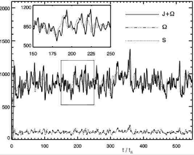
Figure 4.— Run A: The integrated Poynting flux $S$ dynamically balances the Ohmic ($J$) and viscous ($\Omega$) dissipation. Inset shows a magnification of total dissipation and $S$ for $150\leq t/\tau_{\mathcal{A}}\leq 250$.

The phenomenology described in this section is general and we have found it in all the simulations that we have performed, in particular we have always found that in the nonlinear stage a statistical steady state is reached where energies fluctuate around a mean value and total dissipation and Poynting flux on the average balance while on small timescales decorrelate. In particular, to check the temporal stability of these features, which are fully confirmed, we have performed a numerical simulation (run C) with the same parameters as run A, but with a lower resolution (128x128x100), a Reynolds number $Re=200$ and a longer duration ($t\sim 2,000\,\tau_{\mathcal{A}}$). On the opposite the average levels of the energies and of total dissipation depend on the parameters used as we describe in the next sections.

Before describing these features, in the next section we describe the current sheets formation, their temporal evolution and other properties.

4.1.1 Current Sheets, Magnetic Reconnection, Global Magnetic Field Topology and Self-Organization

The nonlinear stage is characterized by the presence of current sheets elongated along the axial direction (Figures (18a)-(18b)), which exhibit temporal dynamics and are the dissipative structures of the system. We now show that they are the result of a nonlinear cascade. Figure 6 shows the time evolution of the first 11 modes of magnetic energy for the first 20 crossing times $\tau_{\mathcal{A}}$ for run A. During the linear stage the magnetic field is given by eq. (24) and is the mapping of the difference between the top ($z=10$) and bottom ($z=0$) photospheric velocities $\mathbf{u}^{L}(x,y)-\mathbf{u}^{0}(x,y)$, whose streamlines are shown in Figure 17a. The field lines of the orthogonal magnetic field in the midplane ($z=5$) at time $t=0.63\,\tau_{\mathcal{A}}$ are shown in Figure 17b, and as expected they map the velocity field. The same figure shows in colour the axial current $j$. As shown by eq. (24) (taking the curl) the large scale motions that we have imposed at the photosphere induce large scale currents in all the volume and, as described in the previous section, if there was not a nonlinear dynamics a balance between diffusion and forcing would be reached, where no small scale would be formed and the magnetic field would always map the photospheric velocities.

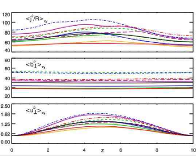
Figure 5.— Run A: 2D averages in the x-y planes of the ohmic dissipation $j^{2}/Re$, the magnetic and velocity fields $\mathbf{b}_{\perp}^{2}$, and $\mathbf{u}_{\perp}^{2}$, as a function of z. The different colours represent 10 different times separated by $\Delta t=50\,\tau_{\mathcal{A}}$ in the interval $30\,\tau_{\mathcal{A}}\leq t\leq 480\,\tau_{\mathcal{A}}$.

As time proceeds the magnetic field grows and a cascade transfers energy from the large scales, where the photospheric forcing (10) injects energy at the wavenumbers $n=3$ and $4$, to the small scales (Figure 6). In physical space this cascade corresponds to the collapse of the large scale currents which lead to the formation of current sheets, as shown in Figures 17c and 17d. In Figures 17e and 17f we show the magnetic field lines at time $t=18.47\,\tau_{\mathcal{A}}$, in the fully nonlinear stage, with respectively the axial component of the current $j$ and of the vorticity $\omega$. The resulting magnetic topology is quiet complex, X and Y-points are not in fact easily distinguished. They are distorted and very often a component of the magnetic field orthogonal to the current sheet length is present, so that the sites of reconnection are more easily identified by the corresponding vorticity quadrupoles. As shown in Figures 17e and 17f, the more or less distorted current sheets are always embedded in quadrupolar structures for the vorticity, a characteristic maintained throughout the whole simulation, and a clear indication that nonlinear magnetic reconnection is taking place.

Figures 18a and 18b show a view from the side and the top of the 3D current sheets at time $t=18.47\,\tau_{\mathcal{A}}$. When looked from the side the current sheets, which are elongated along the axial direction, look space filling, but the view from the top shows that the filling factor is actually small (see also Figure 17).

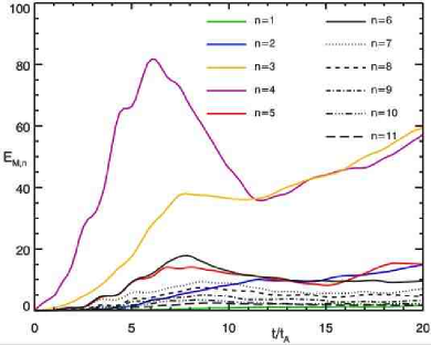
Figure 6.— Run A: First 11 magnetic energy modes as a function of time covering the first 20 Alfvén crossing times $\tau_{\mathcal{A}}$. Photospheric motions inject energy at $n=3$ and $4$.

Another aspect of the dynamics is self-organization: while until time $t=4.79\,\tau_{\mathcal{A}}$ the magnetic field lines are still approximately a mapping of the photospheric velocities, in the fully nonlinear stage they depart from it and have an independent topology that evolves dynamically in time (see the associated movie for the time evolution covering $40$ crossing times from $\sim 508\,\tau_{\mathcal{A}}$ up to $\sim 548\,\tau_{\mathcal{A}}$; notations and simulation are the same used in Figure 17). The reason for which the photospheric forcing does not determine the spatial shape of the magnetic field lines is due to the bigger value of the rms of the magnetic field $b_{\perp}=<\mathbf{b}_{\perp}^{2}>^{1/2}$ in the volume respect to the rms of the photospheric forcings $u_{ph}=<(\mathbf{u}_{\perp}^{0}-\mathbf{u}_{\perp}^{L})^{2}>^{1/2}\sim 1$ (eqs. (16)-(17)).

This means that the contribution to the dynamics of the Alfvénic perturbations propagating from the boundary are much smaller, over short periods of time, than the self-consistent non-linear evolution due to the magnetic fields inside the domain, and therefore can not determine the topology of the magnetic field. For run A and G, both with $c_{\mathcal{A}}=200$, the ratio is $b_{\perp}/u_{ph}\sim 6$ and it increases up to $b_{\perp}/u_{ph}\sim 27$ in run I with $c_{\mathcal{A}}=1000$. On the other hand these waves continuously transport from the boundaries the energy that sustain the system in a magnetically dominated statistically steady state.

All the facts presented in this section, and the properties of the cascade and of the resulting current sheets in presence of a magnetic guide field outlined in § 5, lead to the conclusion that the current sheets do not generally result directly from a geometrical misalignment of neighboring magnetic field lines stirred by their footpoints motions, but that they are the result of a nonlinear cascade in a self-organized system.

Although the magnetic energy dominates over the kinetic energy, the ratio of the rms of the orthogonal magnetic field over the axial dominant field $B_{0}$ is quite small. For $c_{\mathcal{A}}=200,400$ and $1000$ it is $\sim 3\%$, so that the average inclination of the magnetic fieldlines respect to the axial direction is just $\sim 2^{\circ}$, it is only for the lower value $c_{\mathcal{A}}=50$ that $b_{\perp}/B_{0}\sim 4\%$ and the angle is $\sim 4^{\circ}$. The field lines of the total magnetic field at time $t=18.47\tau_{\mathcal{A}}$ are shown in Figures 18c and 18d. The computational box has been rescaled for an improved viewing, and to attain the original aspect ratio the box should be stretched 10 times along the axial direction. The magnetic topology for the total field is quiete simple, as the line appear slightly bended. It is only in correspondence of the small scale current-sheets that field lines on the opposite side may show a relative inclination. But as the current sheets are very tiny (and their width decreases at higher Reynolds numbers), they occupy only a very small fraction of the volume, so that the bulk of the magnetic field lines appears only slightly bended.

It is often suggested, or implicitly assumed, that current sheets are formed because the magnetic field line footpoints are subject to a random walk. The complexity of the footpoint trajectory would then be a necessary ingredient. In fact it would give rise to a complex topology for the coronal magnetic field, leading either to tangled field lines which would then release energy via fast magnetic reconnection, or to turbulence. So that the “complexity” of the footpoint motions would be responsible for the “complex” dynamics in the corona.

On the opposite our simulations show that this system in inherently turbulent, and that “simple” footpoint motions give rise to turbulent dynamics characterize by the presence of an inertial range (§ 5) and dynamical current sheets. In fact our photospheric forcing velocities (Figures 1-2) are constant in time and have only large-scale components (eq. (10)), so that the footpoint motions are “ordered” and do not follow any random walk. During the linear stage this gives rise to a magnetic field that grows linearly in time (eq. (24)) and that is a mapping of the velocity fields (see eq. (24) and Figures 17a and 17b), i.e. both the magnetic field and the current have only large-scale components. The footpoint motions of our photospheric velocities never bring two magnetic field lines close to one another, i.e. they never geometrically produce a current sheet. Current sheets are produced on an ideal timescale, the nonlinear timescale, by the cascade. Furthermore, as we show in the next section, the statistically steady state that characterizes the nonlinear stage results from the balance at the large-scales between the injection of energy and the flow of this energy from the large scales toward the small scales, where it is finally dissipated.

As the system is self-organized and the magnetic energy increases at higher values of the axial magnetic fields, very likely different static or time-dependent (with the characteristic photospheric time $\sim 300\,s$) forcing functions, will not be able to determine the spatial shape of the orthogonal magnetic field. In our more realistic simulation with $c_{A}=1000$ the ratio $b_{\perp}/u_{ph}$ is in fact $\sim 27$. Other forcing functions are currently being investigated, and time-dependent forcing functions are likely to modulate with their associated timescale the rms of the system, like total energy and dissipation.

5. TURBULENCE

Before analyzing in detail further aspects of our simulations, namely inertial spectra, anisotropies and scaling laws, let us briefly justify the statement that the time-dependent Parker problem, i.e. the dynamics of a magnetofluid threaded by a strong axial field whose footpoints are stirred by a velocity field, is an MHD turbulence problem.

The fact that at the large orthogonal scales the Alfvén crossing time $\tau_{\mathcal{A}}$ is the fastest timescale so that during the linear stage the fields evolves as  (24)-(25), means that the photosphere’s role is to contribute an anisotropic magnetic forcing function that stirs the fluid, with an orthogonal length typical of the convective cells ($\sim 1000\,km$) and an axial length is given by the loop length $L$.

Typically, forced MHD turbulence simulations (e.g. see Biskamp (2003) and references therein) are performed using a 3-periodic numerical cube with a volumetric forcing function which mimics some physical process injecting energy at the large scales.

Solutions (24)-(25) can be approximately obtained introducing themagnetic forcing function $\mathbf{F}_{m}$ in equation (2)

$$\mathbf{F}_{m}=\frac{\mathbf{u}^{L}(x,y)-\mathbf{u}^{0}(x,y)}{\tau_{\mathcal{A}}},$$ (38)

and implementing 3-periodic boundary conditions in our elongated ($0\leq x,y\leq 1$, $0\leq z\leq L$) computational box. During the linear stage this forcing would give rise, apart from the small velocity field (25), to the same magnetic field. During the nonlinear stage, as $\tau_{A}<\tau_{nl}$, it would still give rise to a similar injection of energy. This property was the basis for the body of previous 2D calculations (Einaudi et al., 1996; Dmitruk et al., 1998; Georgoulis et al., 1998)

In particular the photospheric motions imposed at the boundaries for the Parker problem take the place of, and represent a different physical realizations of the forcing function generally used for the 3-periodic MHD turbulence box. In the Parker model, the equivalent forcing stirs the magnetic field, whiile in standard simulations the forcing stirs both velocity and magnetic fields or mostly the velocity field. The main differences between “standard” MHD turbulence simulations and the problem at hand are that a) the peculiarity of the low-frequency photospheric forcing leads to magnetic energy largely dominating over the kinetic energy in the system b) the forcing involves line-tying of the magnetic field with 3-periodic boundary conditions. Line-tying inhibit the inverse cascade for the magnetic field, as described later in this section (§ 5.4). Equivalently, one may say that line-tying hinders magnetic reconnection by rendering it less energetically favorable due to the increased field line-curvature it requires compared to the unbound system. This property is fundamental to the anomalous scaling laws and enhanced overall heating rates that will be found below.

In MHD, the cascade takes place preferentially in planes orthogonal to the local mean magnetic field (Shebalin et al. (1983)). The small scales formed are not uniformly distributed in this plane, rather they are organized in dynamical current-vortex sheets extended along the direction of the local main field. These current sheets with associated quadrupolar vorticity filaments form the dissipative structures of MHD turbulence (e.g. Biskamp & Müller (2000), Biskamp (2003) and references therein). In our case, because the axial field is strong, the current sheets are elongated along the axial direction to the point of being quasi-uniform along the loop axis (Figure 18).

5.1. Spectral Properties

In order to investigate inertial range spectra, we have carried out four simulations (runs F, G, H and I in Table 1) with a resolution of 512x512x200 grid points using a mild power ($n=4$) for hyperdiffusion (12)-(13).

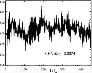
Figure 7.— Run G: Ratio between cross-helicity $H^{C}$ and total energy $E$ as a function of time. $H^{C}\ll E$ shows that the system is in a regime of balanced turbulence.

In turbulence the fundamental physical fields are the Elsässer variables $\mathbf{z}^{\pm}=\mathbf{u}_{\perp}\pm\mathbf{b}_{\perp}$. Their associated energies

$$E^{\pm}=\frac{1}{2}\int\!\mathrm{d}V\,\left(\mathbf{z}^{\pm}\right)^{2},$$ (39)

are linked to kinetic and magnetic energies $E_{K}$, $E_{M}$ and to the cross helicity $H^{C}$

$$H^{C}=\frac{1}{2}\int\!\mathrm{d}V\,\mathbf{u}_{\perp}\cdot\mathbf{b}_{\perp}$$ (40)

by

$$E^{\pm}=E_{K}+E_{M}\pm H^{C}$$ (41)

Nonlinear terms in equations (12)-(15) are symmetric under the exchange $\mathbf{z}^{+}\leftrightarrow\mathbf{z}^{-}$, so as substantially are also boundary conditions (16)-(17), given that the two forcing velocities are different but have the same rms values ($=1/\sqrt{2}$). It is then expected that $H^{C}\ll E$ so that none of the two energies prevails $E^{+}\sim E^{-}\sim E$, where $E=E_{K}+E_{M}$ is total energy. In Figure 7 the ratio $H^{C}/E$ is shown as a function of time for run G. Cross helicity has a maximum value of 5% of total energy, and its time average is $\sim 1\%$, and similar values are found for all the simulations. Furthermore perpendicular spectra of $E$ and $E^{\pm}$ in simulations F, G, H and I, overlap each other, so that as expected we can also assume that

$$\delta z^{+}_{\lambda}\sim\delta z^{-}_{\lambda}\sim\delta z_{\lambda},$$ (42)

where $\delta z_{\lambda}$ is the rms value of the Elsässer fields $\mathbf{z}^{\pm}$ at the perpendicular scale $\lambda$.

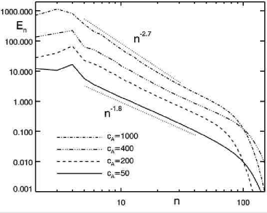
Figure 8.— Total energy spectra as a function of the wavenumber $n$ for simulations F, G, H and I. To higher values of $c_{\mathcal{A}}=v_{\mathcal{A}}/u_{ph}$, the ratio between the Alfvén and photospheric velocities, correspond steeper spectra, with spectral index respectively $1.8$, $2$, $2.3$ and $2.7$.

In the following we always consider the spectra in the orthogonal plane $x$-$y$ integrated along the axial direction $z$, unless otherwise noted. Furthermore as they are isotropic in the Fourier $k_{x}$-$k_{y}$ plane, we will consider the integrated 1D spectra, so that for total energy

$$E=\frac{1}{2}\,\int_{0}^{L}\!\mathrm{d}z\,\iint_{0\ \ \ }^{\ell\ \,}\displaylimits\!\mathrm{d}x\,\mathrm{d}y\,\left(\boldsymbol{u}^{2}+\boldsymbol{b}^{2}\right)=\\ =\frac{1}{2}\,\int_{0}^{L}\!\mathrm{d}z\,\ell^{2}\sum_{\boldsymbol{k}}\left(|\boldsymbol{\hat{u}}|^{2}+|\boldsymbol{\hat{b}}|^{2}\right)\left(\boldsymbol{k},z\right)=\sum_{n}E_{n},\\ n=1,2,\dots$$ (43)

where, similarly to eq. (10), $n$ indicates “rings” in $k$-space. Figure 8 shows the total energy spectra $E_{n}$ averaged in time, obtained from the hyperdiffusive simulations F, G, H and I with dissipativity $n=4$ (eqs. (12)-(13)) and respectively $c_{\mathcal{A}}=50$, $200$, $400$ and $1000$. An inertial range displaying a power law behaviour is clearly resolved. The spectra visibly steepens increasing the value of $c_{\mathcal{A}}$, with spectral index ranging from $1.8$ for $c_{\mathcal{A}}=50$ up to $\sim 2.7$ for $c_{\mathcal{A}}=1000$. The spectra are clearly always steeper than the well known (strong) MHD inertial range turbulence spectra $k_{\perp}^{-5/3}$ or $k_{\perp}^{-3/2}$ .

This steepening is certainly not a numerical artifact: the use of hyperdiffusion gives rise to a hump at high wave-number values, known as the bottleneck effect (Falkovich, 1994), which when present flattens the spectra. Furthermore we use the same value of dissipativity ($n=4$) used by Maron & Goldreich (2001), who find the same IK spectral slope ($-3/2$), also confirmed in recent higher-resolution simulations performed by Müller & Grappin (2005) with standard $n=1$ diffusion.

In our simulations, a hump or flattening at high wavenumbers is best visible in run H with $c_{\mathcal{A}}=400$, which might be due to the bottleneck effect, but a more probable interpretation involves a transition from weak to strong turbulence at the smaller scales within the inertial range, which requires a preliminary discussion of strong vs. weal turbulence in MHD.

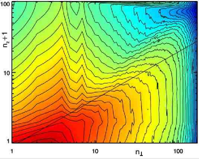
Figure 9.— Run I: Snapshot of the 2D spectrum $E(n_{\perp},n_{z})$ in bilogarithmic scale at time $t\sim 145\,\tau_{\mathcal{A}}$. $n_{\perp}$ and $n_{z}$ are respectively the orthogonal and axial wavenumbers. The 2D spectrum is shown as a function of $n_{\perp}$ and $n_{z}+1$, to allow the display of the $n_{z}=0$ component.

Recently a lot of progress has been made in the understanding MHD turbulence both in the condition of so-called strong (Goldreich & Sridhar, 1995, 1997; Cho & Vishniac, 2000; Biskamp & Müller, 2000; Müller et al., 2003; Müller & Grappin, 2005; Boldyrev, 2005, 2006; Mason et al., 2006) and weak turbulence (Ng & Bhattacharjee, 1997; Goldreich & Sridhar, 1997; Galtier et al., 2000; Galtier & Chandran, 2006). Weak turbulence has been investigated mainly through analytical methods. The total energy spectrum can be characterized by a $k_{\perp}^{-2}$ power law, which is easily found phenomenologically by considering that the Alfvén effect occurs along the field while the cascade proceeds in the orthogonal direction (Ng & Bhattacharjee, 1997). While our MHD simulations, even with our line-tying boundary conditions and anomalous energetic regime ($b$ dominating over $u$ except at the smallest scales), confirm the presence of the $k_{\perp}^{-2}$ spectrum for a range of loop parameters, steeper spectra are also found nearly reaching $k_{\perp}^{-3}$, clearly linked to the strength of the axial field $B_{0}$ an effect we discuss more in detail in the following subsection.

The formation of an inertial range is crucially related to the anisotropy of the cascade, where a relationship between spectral extent in the perpendicular and parallel directions known as “critical balance” may be derived. To understand this feature, consider the timescale $T_{\lambda}$, the energy-transfer time at the corresponding scale $\lambda$, characterizing the nonlinear dynamics at that scale. $T_{\lambda}$ does not necessarily coincide with the eddy turnover time $\tau_{\lambda}=\lambda/\delta z_{\lambda}$ because of the Alfvén effect. Spatial structures along the axial direction result from wave propagation (at the Alfvén speed $c_{\mathcal{A}}$) of the orthogonal fluctuations. In other words, the cascading of turbulence in two different planes separated by a distance $\ell_{\parallel}$ leads to formation of scales in the parallel direction whose smallest size can be (Goldreich & Sridhar, 1995; Cho et al., 2002; Oughton et al., 1994)

$$\ell_{\parallel}(\lambda)\sim c_{\mathcal{A}}T_{\lambda},$$ (44)

the critical balance condition. $T_{\lambda}$ will be smaller at smaller scales, so that smaller perpendicular scales create smaller axial scales.

Figure 9 shows a snapshot at time $t\sim 145\,\tau_{\mathcal{A}}$ of the 2D spectrum $E(n_{\perp},n_{z})$ for run I in bilogarithmic scale, where $n_{z}$ and $n_{\perp}$ are respectively the axial and orthogonal wavenumbers. Consider vertical cuts at $n_{\perp}=const$: it is clearly visible that from $n_{\perp}=1$ up to $n_{\perp}\sim 20$ the wavenumbers with $n_{z}>1$ are scarcely populated compared to the respective wavenumbers with $n_{z}\leq 1$ (the parallel spectrum has also the $n_{z}=0$ component, in Figure 9 the vertical coordinate is $n_{z}+1$). However note also how the loci of maximum parallel wave-number do not precisely follow the critical balance line, rather they are offset at larger $n_{\perp}$: in our case, the hypothetical length of the axial structures (from critical balance) can be longer than the characteristic length of the system, in our case the length of the coronal loop $L$. But in the range of perpendicular wavenumbers for which

$$\ell_{\parallel}(\lambda)>L,$$ (45)

boundary conditions, i.e. line-tying, intervenes and the cascade along the axial direction is strongly inhibited. In our simulations this occurs roughly at $n_{\perp}\sim 20$. Beyond $n_{\perp}\sim 20$ the spectrum is roughly constant along $n_{\perp}=const$ up to a critical value where it drops.

Interestingly enough, the slope of the 1D spectrum for run I (Figure 8) diminishes its value around $n_{\perp}\sim 20$. The reason is that the condition $\ell_{\parallel}(\lambda)>L$ with $\ell_{\parallel}(\lambda)$ defined by critical balance, turns out to play a major role in the “strength” or “weakness” of the cascade: for $n_{\perp}\lesssim 20$ the system is in a weak turbulent regime, while for $n_{\perp}\gtrsim 20$ a transition to strong turbulence is observed.

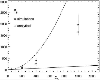
Figure 10.— Total energy at the injection scale (modes 3 and 4), time-averaged for the four simulations F, G, H and I with different Alfvén velocities. The dashed line shows the curve $E_{in}\propto c_{\mathcal{A}}^{2}$, while the continuous line shows $E_{in}$ as a function of $c_{\mathcal{A}}$ as obtained from equation (66) for $\alpha=0$ corresponding to a Kolmogorov spectrum. The actual growth of $E_{in}$, both simulated and derived from (66), show that the growth is less than quadratical but higher than in the simple Kolmogorov case.

In our runs, larger values of $c_{\mathcal{A}}$, i.e. of the parameter $f$ (18), lead to larger magnetic energy and total energies, while the kinetic energy remains smaller than magnetic energy and increases much less (increasing its value by a factor of $6$ from $c_{\mathcal{A}}=50$ to $c_{\mathcal{A}}=1000$). In particular Figure 10 shows total energy at the injection scales (see § 2.2), i.e. the sum of the modes $n=3$ and $n=4$ (see eq. 43) of total energy,

$$E_{in}=E_{3}+E_{4}$$ (46)

as a function of the non-dimensional Alfvén velocity $c_{\mathcal{A}}$. Their growth is less than quadratical in $c_{\mathcal{A}}$, which implies that the rms of the velocity and magnetic fields at the injection scale (or equivalently the Elsässer fields $\delta z_{in}$) grow less than linearly. Hence as $c_{\mathcal{A}}$ is increased, the ratio $\chi$, a measure of the relative strength of the nonlinear interactions at the injection scale, decreases: at different values of $c_{\mathcal{A}}$ different regimes of weak turbulence are therefore realized at the larger scales of the inertial range, as the different spectra in Figure 8 confirm.

The presence of a “double” inertial range, with a weak-type power-law index at larger scales, and a flatter strong-type power-law index at smaller scales would not affect the overall cascade rate, and therefore the scalings of loop heating with loop parameters. These are set at the larger scales, and are therefore dependent on the cascade rate determined by the weak-type scaling law, for which a physically motivated phenomenological derivation is presented below. We stress that the possible existence of a “double” inertial range, surmised here with scaling laws and somewhat tenuous numerical evidence, does not appear to have been predicted before and requires substantiating evidence from higher numerical resolution simulations which are planned for the near future.

5.2. Phenomenology of the Inertial Range and Coronal Heating Scalings

We now introduce a phenomenological model to determine the energy transfer time-scale $T_{\lambda}$ and as a consequence the properties of the cascade. This time-scale, and therefore the different spectra which result, can only depend on the single non-dimensional quantity defining our system, namely $f={\ell_{c}\,v_{\mathcal{A}}}/{L\,u_{ph}}$ (18). The simulations show that as this parameter is increased the spectra steepen leading to a weakened cascade. We revert here to dimensional quantities for the scalings, so that we can quantify the resulting coronal heating rates.

The Alfvén effect is based on the idea that two counterpropagating Alfvén waves interact only for the time $\tau_{\parallel}=\ell_{\parallel}/v_{\mathcal{A}}$, leading to a transfer energy time longer that the “generalized” eddy turnover time

$$\tau_{\lambda}=\frac{\lambda}{\delta z_{\lambda}},$$ (47)

The ratio between these two timescales

$$\chi=\frac{\tau_{\mathcal{A}}}{\tau_{\lambda}}=\frac{\ell_{\parallel}\,\delta z_{\lambda}}{\lambda\,c_{\mathcal{A}}}$$ (48)

gives a measure of their relative strength. Iroshnikov (1964) and Kraichnan (1965) proposed that the energy transfer time $T_{\lambda}$, because of the Alfvén effect, is longer than the eddy turnover time, and is given by

$$T_{\lambda}\sim\tau_{\lambda}\,\frac{\tau_{\lambda}}{\tau_{A}},$$ (49)

where however they considered an isotropic situation, so that the Alfvén time was given by the propagation time over the scale of the Alfvénic packet. For weak turbulence however $\ell_{\parallel}>L$, so that the Alfvén time must be based on the scale $L$: $\tau_{\mathcal{A}}=L/v_{\mathcal{A}}$.

In addition, we must allow line-tying which acts to slow the destruction of eddies on a given scale ${\lambda}$ more effectively than the standard random encounter effect ${\tau_{\lambda}}/{\tau_{A}}$ (Dobrowolny et al., 1980). We can therefore assume a sub-diffusive behaviour for ${\bf z^{+}}---{\bf z^{-}}$ non-linear encounters leading to

$$T_{\lambda}\sim\tau_{\lambda}\,\left(\frac{\tau_{\lambda}}{\tau_{A}}\right)^{\alpha},$$ (50)

with values $\alpha>1$ and depending in some way on the parameter $f$ [recall that $\alpha=0,1$ correspond respectively to anisotropic Kolmogorov and Kraichnan cases (the latter leading to a $k^{-2}$ inertial range spectrum)].

Our simulations then close this ansatz by determining how $alpha$ depends on $f$: integrating over the whole volume ($\ell\times\ell\times L$), the energy cascade rate may now be written as

$$\epsilon\sim\ell^{2}\,L\,\rho\,\frac{{\delta z_{\lambda}}^{2}}{T_{\lambda}},$$ (51)

Using (50) the energy transfer rate is given by

$$\epsilon\sim\ell^{2}L\cdot\rho\,\frac{\delta z_{\lambda}^{2}}{T_{\lambda}}\sim\ell^{2}L\cdot\rho\,\left(\frac{L}{v_{A}}\right)^{\alpha}\,\frac{\delta z_{\lambda}^{\alpha+3}}{\lambda^{\alpha+1}}.$$ (52)

Identifying, as usual, the eddy energy with the band-integrated Fourier spectrum $\delta z^{2}_{\lambda}\sim k_{\perp}E_{k_{\perp}}$, where $k_{\perp}\sim\ell/\lambda$, from eq. (52) we obtain the spectrum

$$E_{k_{\perp}}\propto k_{\perp}^{-\frac{3\alpha+5}{\alpha+3}},$$ (53)

where for $\alpha=0,1$ the $-5/3,-3/2$ slope for the anisotropic Kolmogorov, Kraichnan spectra are is recovered, but steeper spectral slopes up to an asymptotic value of $-3$ are obtained with higher values of $\alpha$.

Correspondingly, from eqs. (51)-(52), the following scaling relations for $\delta z_{\lambda}$ and $T_{\lambda}$ follow:

$$\delta z_{\lambda}\sim\left(\frac{\epsilon}{\ell^{2}L\rho}\right)^{\frac{1}{\alpha+3}}\left(\frac{v_{\mathcal{A}}}{L}\right)^{\frac{\alpha}{\alpha+3}}\ \lambda^{\frac{\alpha+1}{\alpha+3}}$$ (54)

$$T_{\lambda}\sim\left(\frac{\ell^{2}L\rho}{\epsilon}\right)^{\frac{\alpha+1}{\alpha+3}}\left(\frac{v_{\mathcal{A}}}{L}\right)^{\frac{2\alpha}{\alpha+3}}\ \lambda^{2\,\frac{\alpha+1}{\alpha+3}}$$ (55)

Recently Boldyrev (2005) has proposed a similar model, which aims to overcome some discrepancies between previous models and numerical simulations, and that self-consistently accounts for the formation of current sheets, for the cascade of strong turbulence. His energy transfer time is given by

$$T_{\lambda}=\frac{\lambda}{\delta z_{\lambda}}\left(\frac{v_{\mathcal{A}}}{\delta z_{\lambda}}\right)^{\alpha},$$ (56)

but he suggests the interval $0\leq\alpha\leq 1$ as appropriate to strong turbulence.

As pointed out above of § 3, the solutions of equations (12)-(14) depend only on the non-dimensional parameter $f=\ell_{c}\,v_{\mathcal{A}}/L\,u_{ph}$ (eq. (18)) and so $\alpha$ (50) is only a function of $f$

$$\alpha=\alpha\left(\frac{\ell_{c}\,v_{\mathcal{A}}}{L\,u_{ph}}\right).$$ (57)

We estimate the value of $\alpha$ from the slope of the total energy spectra (53), as described in Rappazzo et al. (2007). As shown in Figure 8 to different values of $c_{\mathcal{A}}=v_{\mathcal{A}}/u_{ph}$, (i.e. $f$) ranging from $50$ up to $1000$ correspond spectral slopes from $\sim-1.8$ up to $\sim-2.7$. Thes in turn correspond (through eq. (53)) to values of $\alpha$ ranging from $\sim 0.33$ up to $\sim 10.33$.

How do the above results affect coronal heating scalings? The energy that is injected at the large scales by photospheric motions, and whose energy rate ($\epsilon_{in}$) is given quantitatively by the Poynting flux (21), is transported (without being dissipated) along the inertial range at the rate $\epsilon$ (52), to be finally dissipated at the rate $\epsilon_{d}$. In a stationary state all these fluxes must be equal

$$\epsilon_{in}=\epsilon=\epsilon_{d}$$ (58)

The injection energy rate (21) is given by S, the Poynting flux integrated over the photospheric surfaces:

$$\epsilon_{in}=S=\\ =\rho v_{\mathcal{A}}\left[\int_{z=L}\!\mathrm{d}a\,\left(\boldsymbol{u}_{\perp}^{L}\cdot\boldsymbol{b}_{\perp}\right)-\int_{z=0}\!\mathrm{d}a\,\left(\boldsymbol{u}_{\perp}^{0}\cdot\boldsymbol{b}_{\perp}\right)\right].$$ (59)

2D spatial periodicity in the orthogonal planes allows us to expand the velocity and magnetic fields in Fourier series, e.g.

$$\mathbf{u}_{\perp}\left(x,y\right)=\sum_{r,s}\mathbf{u}_{r,s}\,e^{i\mathbf{k}_{r,s}\cdot\mathbf{x}},$$ (60)

where

$$\mathbf{k}_{r,s}=\frac{2\pi}{\ell}\left(r,s,0\right)\qquad r,s\in\mathbb{Z}$$ (61)

The surface integrated scalar product of $\mathbf{u}_{\perp}$ and $\mathbf{b}_{\perp}$ at the boundary is then given by

$$\int\!\mathrm{d}a\,\boldsymbol{u}_{\perp}\cdot\boldsymbol{b}_{\perp}=\sum_{r,s}\boldsymbol{u}_{r,s}\cdot\int_{0}^{\ell}\!\!\!\int_{0}^{\ell}\mathrm{d}x\mathrm{d}y\ \boldsymbol{b}_{\perp}e^{i\boldsymbol{k}_{r,s}\cdot\boldsymbol{x}}=\\ =\ell^{2}\,\sum_{r,s}\boldsymbol{u}_{r,s}\cdot\boldsymbol{b}_{-r,-s},\qquad r,s\in\mathbb{Z}$$ (62)

This integral is clearly dominated by large scales consistent with observations of photospheric motions. In our case (eq. (10)) boundary velocities only have components for wave numbers $(r,s)\in\mathbb{Z}^{2}$ with absolute values between $3$ and $4$, $3\leq\left(r^{2}+s^{2}\right)^{1/2}\leq 4$. Then in (62) only the corresponding components of $\mathbf{b}_{\perp}$ are selected.

At the injection scale, which is the scale of convective motions $\ell_{c}\sim 1,000\,km$, a weak turbulence regime develops, so that the cascade along the axial direction $z$ is limited and in particular the magnetic field $\mathbf{b}_{\perp}$ can be considered approximately uniform along $z$ at the large orthogonal scales. Then from eq. (59) we obtain

$$\epsilon_{in}=S\sim\rho v_{\mathcal{A}}\int\!\mathrm{d}a\,\left(\mathbf{u}_{\perp}^{L}-\mathbf{u}_{\perp}^{0}\right)\cdot\mathbf{b}_{\perp}$$ (63)

Introducing $\mathbf{u}_{ph}=\mathbf{u}_{\perp}^{L}-\mathbf{u}_{\perp}^{0}$, using relation (62), and integrating over the surface, we can now write

$$\epsilon_{in}=S\sim\ell^{2}\rho v_{\mathcal{A}}u_{ph}\delta z_{\ell_{c}},$$ (64)

where we have approximated the value of $\delta b_{\ell_{c}}$, the rms of the magnetic field at the injection scale $\ell_{c}$, with the rms of the Elsässer variable because the system is magnetically dominated, i.e. $\delta z_{\ell_{c}}=\left(\delta u^{2}_{\ell_{c}}+\delta b^{2}_{\ell_{c}}\right)^{1/2}\sim\delta b_{\ell_{c}}$.

We now have an expression for $\epsilon_{in}$, where the only unknown variable is $\delta z_{\ell_{c}}$, as $\ell_{c}$, $\rho$, $v_{\mathcal{A}}$ and $u_{ph}$ are the parameters characterizing our model of a coronal loop.

The transfer energy rate $\epsilon$ does not depend on $\lambda$. Considering then $\lambda=\ell_{c}$ in equation (52), we have

$$\epsilon\sim\frac{\rho\,\ell^{2}L^{\alpha+1}}{\ell_{c}^{\alpha+1}\,v_{A}^{\alpha}}\,\delta z_{\ell_{c}}^{\alpha+3}.$$ (65)

Equations (64) and (65) show another aspect of self-organization. Both $\epsilon_{in}$ and $\epsilon$, respectively the rate of the energy flowing in the system at the large scales, and the rate of the energy flowing from the large scales toward the small scales depend on $\delta z_{\ell_{c}}$, the rms of the fields at the large scale. This shows that the energetic balance of the system is determined by the balance of the energy fluxes $\epsilon$ and $\epsilon_{in}$ at the large scales. The small scales will then dissipate the energy that is transported along the inertial range (see eq. (58)). This implies that beyond a numerical threshold total dissipation (dissipation integrated over the whole volume) is independent of the Reynolds number. In fact beyond a value of the Reynolds number for which the diffusive time at the large scale is negligible, i.e. when the resolution is high enough to resolve an inertial range, the large-scale balance between $\epsilon$ and $\epsilon_{in}$ is no longer influenced by diffusive processes. Of course this threshold is quite low respect to the high values of the Reynolds numbers for the solar corona, but it is still computationally very demanding.

An analytical expression for the coronal heating scalings may be obtained from (64) and (65) yielding the value of $\delta z_{\ell_{c}}^{\ast}$ for which the balance $\epsilon_{in}=\epsilon$ is realized:

$$\frac{\delta z_{\ell_{c}}^{\ast}}{u_{ph}}\sim\left(\frac{\ell_{c}v_{A}}{Lu_{ph}}\right)^{\frac{\alpha+1}{\alpha+2}}$$ (66)

Substituting this value in (65) or equivalently in (64) we obtain the energy flux

$$S^{\ast}\sim\ell^{2}\rho\,v_{A}u_{ph}^{2}\left(\frac{\ell_{c}v_{A}}{Lu_{ph}}\right)^{\frac{\alpha+1}{\alpha+2}}.$$ (67)

As stated in (58) in a stationary cascade all energy fluxes are equal on the average. $S^{\ast}$ is then the energy that for unitary time flows through the boundaries in the coronal loop at the convection cell scale, and that from these scales flows towards the small scales. This is also the dissipation rate, and hence the coronal heating scaling, i.e. the energy which is dissipated in the whole volume for unitary time. As shown in equation (57) the power $\alpha$ depends on the parameters of the coronal loop, and its value is determined numerically with the aforementioned technique.

The observational constraint with which to compare our results is the energy flux sustaining an active region. The energy flux at the boundary is the axial component of the Poynting vector $S_{z}$ (see § 3.1). This is obtained dividing $S^{\ast}$ (67), the Poynting flux integrated over the surface, by the surface $\ell^{2}$:

$$S_{z}=\frac{S^{\ast}}{\ell^{2}}\sim\rho\,v_{A}u_{ph}^{2}\left(\frac{\ell_{c}v_{A}}{Lu_{ph}}\right)^{\frac{\alpha+1}{\alpha+2}},$$ (68)

where $\alpha$ is not a constant, but a function of the loop parameters (57). The exponent in (68) goes from $0.5$ for $\alpha=0$ up to the asymptotic value $1$ for larger $\alpha$. We determine $\alpha$ numerically, measuring the slope of the inertial range (Figure 8), and inverting the spectral power index (53). We have used simulations F, G, H and I to compute the values of $\alpha$, because they implement hyperdiffusion, resolve the inertial range, and then are beyond the numerical threshold below which total dissipation does not depend on the Reynolds number. These simulations implement $v_{\mathcal{A}}=50$, $200$, $400$ and $1,000$, and the corresponding $\alpha$ are $\sim 0.33$, $1$, $3$, $10.33$. The corresponding values for the power $(\alpha+1)/(\alpha+2)$ (68) are $\sim 0.58$, $0.67$, $0.8$ and $0.91$, close to the asymptotic value $1$. $S_{z}$ is shown in Figure 11 (diamond points) as a function of the axial Alfvén velocity $v_{\mathcal{A}}$. To compute the value of $S_{z}$ for $v_{\mathcal{A}}=2,000\,km\,s^{-1}$ we have estimated $\alpha\sim.95$, although for values close to $1$ $S_{z}$ does not have a critical dependence on the value of the exponent.

In Figure 11 we compare the analytical function $S_{z}$ (68) with the respective value determined from our numerical simulations (star points), i.e. with the total dissipation rate by the surface and converted to dimensional units ($(J+\Omega)/\ell^{2}$, see (37)). For the numerical simulation values, the error-bar is defined as 1 standard deviation of the temporal signal. The analytical and computational values are in good agreement for all the 4 simulations considered, and for the more realistical value $v_{\mathcal{A}}=2,000\,km\,s^{-1}$ the dissipated flux is $\sim 1.6\times 10^{6}\,erg\,cm^{-2}\,s^{-1}$. This value is in the lower range of the observed constraint $10^{7}\,erg\,cm^{-2}\,s^{-1}$.

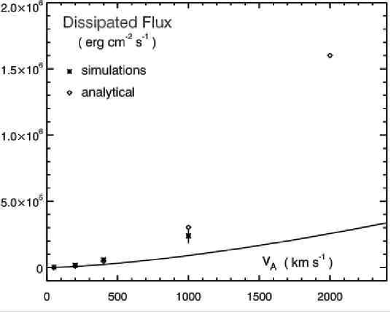
Figure 11.— Analytical (68) and numerically computed dissipated flux as a function of the axial Alfvén velocity $v_{\mathcal{A}}$. The continuous line shows the Poynting flux (68) as a function of $v_{\mathcal{A}}$ in the case $\alpha=0$, corresponding to a Kolmogorov-like cascade. To higher values of $v_{\mathcal{A}}$ correspond a higher dissipation rate because a weak turbulence regime develops.

The continuous line in Figure 11 corresponds to the function $S_{z}$ for $\alpha=0$ (which is approximately realized for $v_{\mathcal{A}}\lesssim 50\,km\,s^{-1}$), in correspondence of which a Kolmogorov spectrum would be present, and $S_{z}\propto v_{\mathcal{A}}^{3/2}$. The computed and analytical values of $S_{z}$ for higher $v_{\mathcal{A}}$ are always beyond this curve, because $\alpha$ increases its values, and a more efficient dissipation takes place. This is due to the fact that to higher values of $\alpha$ correspond higher values of the energy transfer time, and consequently a longer linear stage, higher values of the fields at the large scales (66), and hence a higher value of the energy rates (see (64), (65) and (67)). So that it is realized the only apparently paradox that to a weaker turbulent regime, to which corresponds less efficiency in the nonlinear terms, corresponds a higher total dissipation.

In the last paragraph of § 3.1 we have shown that when the condition (23) is satisfied the emerging flux can be neglected. But in eq. (23) we have to specify the value of the magnetic field $b_{\perp}^{turb}$ self-consistently generated by the non-linear dynamics. This value is given by (66) as the magnetic field dominates ($\delta z^{\ast}_{\ell_{c}}\sim b_{\perp}^{turb}$). By substitution we can now estimate that the emerging flux is negligible when the emerging component of the magnetic field satisfies

$$b_{\perp}^{ef}<B_{0}\,\sqrt{\left(\frac{\ell_{c}}{L}\right)^{\frac{\alpha+1}{\alpha+2}}\left(\frac{u_{ph}}{v_{\mathcal{A}}}\right)^{\frac{1}{\alpha+2}}}$$ (69)

In the asymptotic state $\alpha\gg 1$ the condition reduces to $b_{\perp}^{ef}/B_{0}<\sqrt{\ell_{c}/L}$. For a coronal loop with $L\sim 40,000\,km$, as $\ell_{c}\sim 1,000\,km$ this implies that emerging flux does not play a role if $b_{\perp}^{ef}/B_{0}<1/6$.

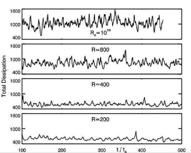
Figure 12.— Transition to turbulence: Total ohmic and viscous dissipation as a function of time for simulations A, B, C, G (displayed on the same scales). All the simulations implement $c_{\mathcal{A}}=200$, but different Reynolds numbers, from $Re=200$ up to $800$. Run G implements hyperdiffusion. For Reynolds numbers lower than $100$ the signal is completely flat and displays no dynamics, at higher Reynolds smaller temporal structures are present.

5.3. Transition to Turbulence and Dissipation vs. Reynolds Number

Turbulence is a characteristic of high Reynolds number systems (e.g. Frisch (1995)). For a sufficiently high viscosity nonlinear dynamics is strongly suppressed, and our system relaxes to a diffusive equilibrium (§3.3), and no significant small scale is formed. Increasing the Reynolds number, the diffusive time at the injection scale (6) $\tau_{d}\sim Re\,\ell_{c}^{2}$ increases. At a certain point it will be big enough not to influence the dynamics as the large scales, an inertial range will then be resolved and total dissipation will not depend any longer from the Reynolds numbers. In fact for higher values of $Re$ the intertial range will extend to higher wave-numbers, but the energy flux will remain the same.

At higher Reynolds numbers smaller scales are resolved, and each scale will contribute with its characteristic time $T_{\lambda}$ to the temporal structure of the rms of the system. Figure 12 shows total dissipation as a function of time for simulations A, B, C and G, on the same time interval, and on the same scale. At increasingly higher values of the Reynolds numbers smaller and smaller temporal structures are added to the signal. Ideally the temporal structure of total dissipation at higher Reynolds numbers is well described by shell-model simulations. For smaller values of Re the signal is completely flat (see Figure 13). This behaviour identifies a transition to turbulence.

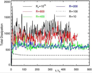
Figure 13.— Total ohmic and viscous dissipation as a function of time for simulations A, B, C, D, E and G, all of them implement $c_{\mathcal{A}}=200$ but different Reynolds numbers. The threshold beyond which dissipation is independent of the Reynolds number can be identified around $Re=800$, corresponding to a numerical resolution of 512x512 points in the orthogonal planes.

Figure 13 shows total dissipation as a function of time for the same 4 simulations shown in Figure 12, plus other 2 simulations at lower Reynolds number, respectively $Re=100$ and $Re=10$ for the complete time interval. For the lowest value of $Re$ no dynamics is present, so that the threshold value for the transition to turbulence can be set to $Re\sim 100$. To higher values of $Re$ dissipation grows. An inertial range is barely solved with a resolution of 512x512 grid points in the $x$-$y$ planes, so that simulation with $Re=800$ can be considered at the threshold. On the other hand simulation G implements hyperdiffusion, so that an inertial range is solved, and the dynamics is not affected by diffusion. The presence of a sufficiently extended inertial range implies in fact that we are beyond the numerical threshold where dissipation does not depend on the Reynolds number (§ 5.2). The threshold value can be identified to a sufficient extent at $Re=800$, i.e. for a numerical grid of 512x512 points. The number of points to use along the axial direction should be enough to allow the formation of all the small scales due to the “critical balance” (Figure 9), but a larger number of points would only result in a waste of computational time.

5.4. Inverse Cascade and Line-tying

Two dimensional simulations (Einaudi et al., 1996; Georgoulis et al., 1998) have shown an inverse cascade for the magnetic energy, corresponding in physical space to the coalescence of magnetic islands. In the 3D case the DC magnetic field along the axial direction is present, giving rise to a field line tension that tends to inhibit an inverse cascade, as motions linked to the coalescence would bend the field lines of the total magnetic field, which are mostly elongated along the axial direction (Figure 18). On the other hand field line tension depends on the strength of the axial field, becoming stronger for a stronger field.

In Figures 14 and 15 the first 4 modes of magnetic energy for simulations F and I, respectively with $c_{\mathcal{A}}=50$ and $1000$, are plotted as a function of time. Energy is injected at wave-numbers $n=3$ and $4$. Modes associated to wave-numbers 1 and 2 grow to higher values than at the injection scale in run F, while in run I they are always limited to lower values. In runs G and H, with respectively $c_{\mathcal{A}}=200$ and $400$ an intermediate behaviour is found, but none of the modes $n=1$ or $2$ never becomes bigger than the injection energy modes.

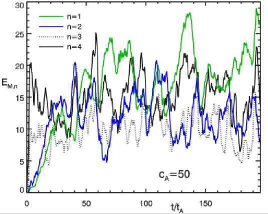
Figure 14.— Run F: In this simulation with $c_{\mathcal{A}}=50$ an inverse cascade at the wavenumbers $n=1$ and $2$ is realized. Energy is injected at wavenumbers $n=3$ and $4$.

5.5. Timescales

In the previous sections we have always affirmed that the Alfvén crossing time $\tau_{\mathcal{A}}=L/v_{\mathcal{A}}$ is the fastest timescale in the system, and that in particular it is smaller than the nonlinear timescale $\tau_{nl}$, which we can identify with the energy transfer time (55) at the injection scale $\tau_{nl}=T_{\ell_{c}}$.

In Figure 3 it is already clear that the nonlinear timescale is longer that $\tau_{\mathcal{A}}$, in fact it shows that the timescale over which energy has substantial variations is bigger than the Alfvén crossing time.

The same behaviour is identified in Figures 14-15, which show the time evolution of the magnetic energy modes for runs F and I. These are more relevant quantities, because to realize a weak MHD turbulence regime it is required that the energy transfer time $T_{\lambda}$ is bigger than the crossing time $\tau_{\mathcal{A}}$ at the injection scale $\lambda=\ell_{c}$ and for a limited range of smaller scales down to some lower bound $\lambda^{\ast}$: $\lambda^{\ast}\leq\lambda\leq\ell_{c}$. The magnetic energy modes at the injection scale ($n=3$ and $4$) change their values on scales bigger than $\tau_{\mathcal{A}}$, and for a larger value of the Alfvén velocity the nonlinear timescale is longer respect to the crossing time (Figures 14-15). We can roughly estimate $\tau_{nl}\sim 5\tau_{\mathcal{A}}$ for run F with $c_{\mathcal{A}}=50$ and $\tau_{nl}\sim 20\tau_{\mathcal{A}}$ for run I with $c_{\mathcal{A}}=1,000$.

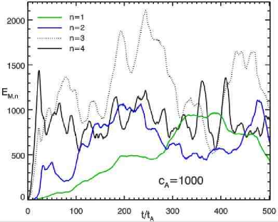
Figure 15.— Run I: Simulation performed with $c_{\mathcal{A}}=1000$. The increased magnetic field line tension inhibits an inverse cascade for the orthogonal magnetic field.

Using our scaling relations we can derive an analytical estimate for the energy transfer time $T_{\lambda}$. Substituting the energy rate (67) in equation (55) we obtain:

$$T_{\lambda}\sim\left(\tau_{\mathcal{A}}\tau_{c}^{\alpha+1}\right)^{\frac{1}{\alpha+2}}\left(\frac{\lambda}{\ell_{c}}\right)^{2\frac{\alpha+1}{\alpha+3}},$$ (70)

where $\tau_{c}=\ell_{c}/u_{ph}$. In particular the ratio over the Alfvén crossing time is:

$$\frac{T_{\lambda}}{\tau_{\mathcal{A}}}\sim\left(\frac{\tau_{c}}{\tau_{\mathcal{A}}}\right)^{\frac{\alpha+1}{\alpha+2}}\left(\frac{\lambda}{\ell_{c}}\right)^{2\frac{\alpha+1}{\alpha+3}},$$ (71)

and as $\tau_{c}>\tau_{\mathcal{A}}$ then self-consistently $T_{\lambda}>\tau_{\mathcal{A}}$. For our loop $\ell_{c}\sim 1,000\,km$ and $u_{ph}\sim 1\,km\,s^{-1}$, so that $\tau_{c}\sim 1,000\,s$. For runs F and I shown in Figures 14 and 15, the loop length is always $L=40,000\,km$, while the Alfvén velocity is respectively $v_{\mathcal{A}}=50$ and $1,000\,km\,s^{-1}$, and the corresponding crossing times $\tau_{\mathcal{A}}=800$ and $40\,s$. Using the values of $\alpha$ computed in §5.2 (respectively $\alpha=0.33$ and $10.33$) we can then roughly estimate from (71), the nonlinear timescale $\tau_{nl}=T_{\lambda=\ell_{c}}$ and its ratio with the Alfvén crossing time:

$$\frac{\tau_{nl}}{\tau_{\mathcal{A}}}=\frac{T_{\ell_{c}}}{\tau_{\mathcal{A}}}\sim\left(\frac{\tau_{c}}{\tau_{\mathcal{A}}}\right)^{\frac{\alpha+1}{\alpha+2}}.$$ (72)

For runs F and I we find $\tau_{nl}/\tau_{\mathcal{A}}=1.2$ and $22.3$ in agreement with the simulations.

Equation (71) can also be used to estimate the extension of the weak turbulence inertial range. The region for which the weak turbulence condition $T_{\lambda}>\tau_{\mathcal{A}}$ is satisfied is:

$$\lambda>\lambda^{\ast}=\ell_{c}\left(\frac{\tau_{\mathcal{A}}}{\tau_{c}}\right)^{\frac{\alpha+3}{2(\alpha+2)}}$$ (73)

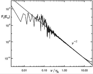
Figure 16.— Temporal spectrum of magnetic energy for run G. $\nu_{\mathcal{A}}=1/\tau_{\mathcal{A}}$ is the frequency corresponding to the Alfvén crossing time. The intermediate part of the spectrum exhibits a $\nu^{-2}$ power law.

Figure 16 shows the temporal spectrum of magnetic energy for run G with $c_{\mathcal{A}}=200$, i.e. we perform the Fourier transform of the magnetic energy as a function of time, and then plot its squared modulus. We use run G because it is the one for which we have saved more frequently the rms quantity and then the plot covers a wider range at high frequencies. The power spectrum is roughly constant up to $\nu/\nu_{\mathcal{A}}\sim 0.2$, which corresponds to $t/\tau_{\mathcal{A}}\sim 5$ in agreement with our scaling (72) which for this case gives $\tau_{nl}/\tau_{\mathcal{A}}\sim 3.3$. Beyond this critical point the power spectrum exhibits a power law which fits $\nu^{-2}$, in agreement with shell-model simulations (Buchlin & Velli, 2007).

6. DISCUSSION AND CONCLUSIONS

We would like first to clarify a few concepts that might otherwise result in misunderstandings of the work that we have presented. The concept of turbulence is used to describe different processes in different research fields, so that its use, without specifications, can result vague and misleading. It is in fact very often used to describe chaotic behaviors at the small scales, often linked to the intermittent dissipation of energy. Although this aspect is present in our simulations, when we say that the Parker problem is an MHD turbulence problem, we refer mainly to the property of turbulence to transfer energy from large to small scales. Namely to its ability to transport the energy from the scale of photospheric motions ($\sim 1000\,km$), where it is injected, down to the small dissipative scales (meters?), without dissipating it at the intermediate scales. This property is clearly identified by the presence of an inertial range with a power law spectrum, which extends from the injection scale to the dissipative scale.

Furthermore turbulence, magnetic reconnection and ohmic heating associated to currents are sometime presented as alternative and/or mutually exclusive coronal heating models. This contraposition is artificial. Current sheets are in fact the dissipative structures of MHD turbulence, and magnetic reconnection at the loci of current sheets is observed in virtually every MHD turbulence simulation in both 2D and 3D (see e.g., Biskamp (2003) and references therein ). Nanoflares are then naturally associated with the time and space intermittency of the small scale deposition of energy (as shown in the 2D case by Georgoulis et al. (1998)), which is due to the cascade which leads to the formation and dissipation of current sheets, and to which we refer collectively with the term MHD turbulence.

In summary, the main results presented in this paper are the following:

• The time-dependent Parker problem may be seen as an MHD turbulence problem, where the large scale forcing function is realized by the photospheric motions.

• This system is genuinely turbulent, in the sense that small scale formation is not driven passively by the random walk of the footpoints, rather it is a property of the maxwell stresses developing in the coronal volume. Current sheets therefore do not generally result directly from a “geometrical” misalignment of neighboring magnetic field lines stirred by their footpoint (random) motions, they are the result of a nonlinear cascade in a self-organized system.

• Nanoflares are naturally associated with the intermittent dissipation of the energy that, injected at the large scales by photospheric motions, is transported to the dissipative scales through a cascade, and is finally dissipated through nonlinear magnetic reconnection.

• Beyond a threshold, that is low compared to the coronal Reynolds numbers, but still computationally very demanding, total dissipation is independent of the Reynolds numbers. This threshold corresponds to a numerical resolution of $\sim 512\times 512$ grid points in the planes orthogonal to the dominant DC magnetic field.

• As the loop parameters vary, different regimes of turbulence develop: strong turbulence is found for weak axial magnetic fields and long loops, leading to Kolmogorov-like spectra in the perpendicular direction, while weaker and weaker regimes (steeper spectral slopes of total energy) are found for strong axial magnetic fields and short loops. There is no single universal scaling law (see (68)), as a consequence the scaling of the heating rate with axial magnetic field intensity, which depends on the spectral index of total energy for given loop parameters, must vary from $B_{0}^{3/2}$ for weak fields to $B_{0}^{2}$ for strong fields at a given aspect ratio.

• For a loop $40,000\,km$ long , with an Alfvén velocity $v_{\mathcal{A}}=2,000\,km\,s^{-1}$ and a numerical density of $10^{10}\,cm^{-3}$, whose footpoints are subject to photospheric motions of $u_{ph}\sim 1\,km\,s^{-1}$ on a scale of $\ell_{c}\sim 1,000\,km$, the energy flux entering the system and being dissipated is $S_{z}\sim 1.6\times 10^{6}\,erg\,cm^{-2}\,s^{-1}$. On the other hand, for a coronal loop typical of a quiet-Sun region, that has the same parameter of the previous case but with a length of $100,000\,km$ and $v_{\mathcal{A}}=500\,km\,s^{-1}$, the resulting Poynting flux is $S_{z}\sim 7\times 10^{4}\,erg\,cm^{-2}\,s^{-1}$.

The most advanced EUV and X-RAY imagers (e.g. those onboard SOHO, TRACE, STEREO and HINODE) have space resolutions ($\sim 800\,km$) of the order of the granulation cells. Hence they do not resolve the small-scales where current sheets, magnetic reconnection and all the dynamical features of the system take place. Their resolution is roughly $1/5$ the length of the perpendicular cross-section of our numerical box ($\sim 4000\,km$). Hence, even if the system is highly dynamical on small-scales (see Figure 17 and the associated movie), integrating over these scales has the effect to “averaging” the small scale dynamics. In particular small scale reconnection cannot be detected, magnetic fieldlines will appear only slightly bended (Figure 18), and their dynamics will appear slower (a modulation of the nonlinear timescale with the thermodinamical timescales).

The topological and dynamical effects associated with magnetic reconnection should be taken into account when modeling the thermodynamical and observational properties of coronal loops (Schrijver, 2007), recalling that most of the dynamics take place at sub-resolution scales while we observe the integrated emission.

Two density current fields that have the same “steady” integrated ohmic dissipation, balanced by a corresponding Poynting Flux (see § 3.3, equation (37) and Figure 4), but with different spatial distributions will have different emissions. Consider the first with only large scale components, as the one that would result from a diffusive process (§ 3.3), while in the second the current has only small scale components, as in the simulations that we have presented. In the second case the filling factor is small (Figures 17 and 18) so that the density of current has a far larger value, and this would correspond to two very different thermodynamical and observational outcomes. But the highly dynamical effects associated with the second case will be averaged and result less dynamical when integrated. Still the integrated observables should be very distinct between the two cases.

Finally, while our simulations give an accurate description of the time-dependent Parker problem, with the limitations on the photospheric forcing field described in the introduction, the use of the reduced MHD equation is justified only for slender loops threaded by a strong axial magnetic field. For short loops, or loops that have orthogonal component of the magnetic field comparable to the axial component, the full set of MHD equation should be implemented. For the slender loops that we have simulated we observe a modest accumulation of energy, which subsequently is released via nanoflares. On the other hand shorter loops, or loops in a more complicated geometry, or subject to loop-loop interactions, and more generally loops affected by the neighboring coronal environment, might exhibit the ability to accumulate more energy (e.g. Low (2006)) and then release it in larger flares, possibly via a “secondary instability” (Dahlburg et al., 2005) or fast magnetic reconnection (Cassak et al., 2006).

Magnetohydrodynamics (MHD) has proved to be a useful tool to investigate the properties of the turbulent cascade (Biskamp, 2003). MHD is very well known to give an approximate description of the plasma dynamics at large scales and low frequencies. In MHD turbulence it is generally supposed that at the small scales a “dissipative mechanism” is present. Most of the properties of the turbulent cascade do not depend on the details of the dissipative mechanism, whether it is described by the diffusive operator present in equations (1)-(2), or more properly by a kinetic mechanism.

In particular in our case, the timescales associated at the scale $\lambda$ ((70) for weak turbulence and (56) for the strong case) decrease for smaller scales. In this way the small-scale dynamics is characterized by high-frequency phenomena, and then it is not well described by MHD, but rather a kinetic model would be more appropriate. It is then possible that (self-consistently) at the small scales particle acceleration plays an important role in the dissipation of energy, a physical process that should be investigated through kinetic models. Nevertheless the coronal heating rates (68), like the cascade properties over an extended range of scales, are independent of the details of the dissipation mechanism. They are determined by the balance, at the large scales (see § 5.2), between the rate of the energy flowing into the loop from the boundaries due to the work done by photospheric motions on the magnetic field line footpoints at the scale of the convective cells, and the rate at which the energy flows along the inertial range from the large scales towards the small scales.

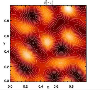
(a)

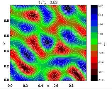
(b)

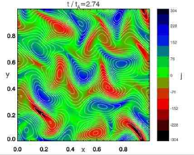
(c)

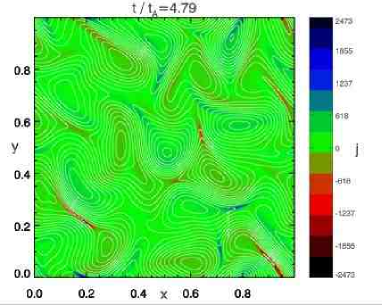
(d)

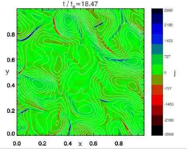
(e)

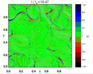
(f)

Figure 17.— Run A: (a) Streamlines of the boundary velocity fields $\mathbf{u}_{\perp}^{0}-\mathbf{u}_{\perp}^{L}$ constant in time. (b)-(e) Axial component of the current $j$ (in color) and field-lines of the orthogonal magnetic field in the mid-plane ($z=5$), at selected times covering the linear and nonlinear regimes up to $t=18.47\,\tau_{\mathcal{A}}$. (f) Axial component of the vorticity $\omega$ (in color) and field-lines of the orthogonal magnetic field in the mid-plane at time $t=18.47\,\tau_{\mathcal{A}}$.
During the linear stage the orthogonal magnetic field is a mapping of the boundary forcing (cfr. a and b). After the collaps of the large-scale currents (b, c, d), which in Fourier space correspond to a cascade of energy (see Figure 6), the topology of the magnetic field departs from the boundary velocity mapping and evolves dynamically in time (see movie). (e)-(f) Current sheets are embedded in quadrupolar vorticity structure, a clear indication of nonlinear magnetic reconnection.

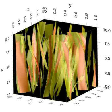
(a)

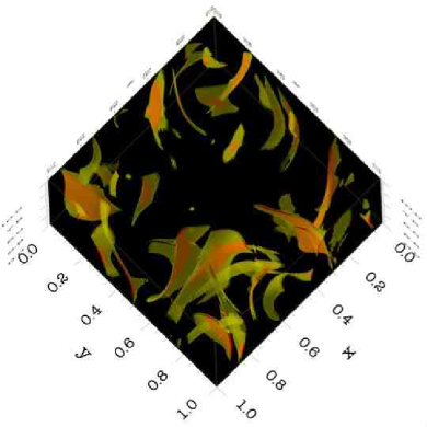
(b)

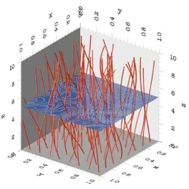
(c)

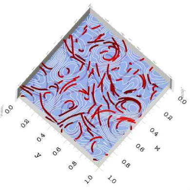
(d)

Figure 18.— Run A: Side (a,c) and top (b,d) views of current sheets (a,b) and field lines of the total magnetic field (c,d) at time $t=18.47\,\tau_{\mathcal{A}}$ (same time as in Figures 17e-17f). For an improved visualization the box size has been rescaled, but the axial length of the computational box is 10 times longer that the perpendicular cross-section length. The rescaling of the box artificially enhances the structures inclination. To restore the original aspect ratio the box should be stretched 10 time along $z$.
(a)-(b) Two isosurfaces of the squared current $j^{2}$. The isosurface at the value $j^{2}=2.8\cdot 10^{5}$ is represented in partially transparent yellow, while red displays the isosurface with $j^{2}=8\cdot 10^{5}$, well below the maximum value of the current at this time $j^{2}_{max}=8.4\cdot 10^{6}$. As typical of current sheets, isosurfaces corresponding to higher values of $j^{2}$ are nested inside those corresponding to lower values. For this reason the red isosurface appears pink. Although from the side view the sheets appear space-filling, the top view shows that the filling factor is small.
(c)-(d) Field-lines of the total magnetic field (orthogonal plus axial), and in the mid-plane ($z=5$) field-lines of the orthogonal component of the magnetic field.

References

- Berger (1991) Berger, M. A. 1991, A&A, 252, 369
- Biskamp (2003) Biskamp, D. 2003, Magnetohydrodynamic Turbulence (Cambridge: Cambridge University Press)
- Biskamp & Müller (2000) Biskamp, D. & Müller, W.-C. 2000, Phys. Plasmas, 7, 4889
- Boldyrev (2005) Boldyrev, S. 2005, ApJ, 626, L37
- Boldyrev (2006) Boldyrev, S. 2006, Phys. Rev. Lett., 96, 115002
- Buchlin & Velli (2007) Buchlin, E. & Velli, M. 2007, ApJ, 662, 701
- Cassak et al. (2006) Cassak, P. A., Drake, J. F. & Shay, M. A. 2006, ApJ, 644, L145
- Cho et al. (2002) Cho, J., Lazarian, A. & Vishniac, E. T. 2002, ApJ, 564, 291
- Cho & Vishniac (2000) Cho, J. & Vishniac, E. T. 2000, ApJ, 539, 273
- Dahlburg et al. (2005) Dahlburg, R. B., Klimchuk, J. A., Antiochos, S. K. 2005, ApJ, 622, 1191
- Dmitruk et al. (1998) Dmitruk, P., Gómez, D. O. & DeLuca, D. D. 1998, ApJ, 505, 974
- Dmitruk & Gómez (1999) Dmitruk, P. & Gómez, D. O. 1999, ApJ, 527, L63
- Dmitruk et al. (2003) Dmitruk, P., Gómez, D. O. & Matthaeus, W. H. 2003, Phys. Plasmas, 10, 3584
- Dobrowolny et al. (1980) Dobrowolny, M., Mangeney, A. & Veltri, P. 1980, Phys. Rev. Lett., 45, 144
- Einaudi et al. (1996) Einaudi, G., Velli, M., Politano, H. & Pouquet, A. 1996, ApJ, 457, L113
- Einaudi & Velli (1999) Einaudi, G. & Velli, M. 1999, Phys. Plasmas, 6, 4146
- Falkovich (1994) Falkovich, G. 1994, Phys. Fluids, 6, 1411
- Frisch (1995) Frisch, U. 2003, Turbulence (Cambridge: Cambridge University Press)
- Galtier et al. (2000) Galtier, S., Nazarenko, S. V., Newell, A. C. & Pouquet, A. 2000, J. Plasma Phys., 63, 447
- Galtier & Chandran (2006) Galtier, S. & Chandran, B. D. G. 2006, Phys. Plasmas, 13, 114505
- Georgoulis et al. (1998) Georgoulis, M. K., Velli, M. & Einaudi, G., 1998, ApJ, 497, 957
- Goldreich & Sridhar (1995) Goldreich, P. & Sridhar, S. 1995, ApJ, 438, 763
- Goldreich & Sridhar (1997) Goldreich, P. & Sridhar, S. 1997, ApJ, 485, 680
- Gomez & Ferro-Fontan (1992) Gomez,D.O. and Ferro-Fontan, C.F. 1992 ApJ, 394, 662
- Grauer and Marliani (2000) Grauer, R. and Marliani, C. 2000, Phys. Rev. Letts., 21, 4850
- Gudiksen & Nordlund (2005) Gudiksen, B. V. & Nordlund, Å. 2005, ApJ, 618, 1020
- Hendrix & Van Hoven (1996) Hendrix, D. L. & Van Hoven, G. 1996, ApJ, 467, 887
- Heyvaerts &Priest (1992) Heyvaerts, J. and Priest, E.R. 1992, ApJ, 390, 297
- Iroshnikov (1964) Iroshnikov, P. S. 1964, Sov. Astron., 7, 566
- Kadomtsev & Pogutse (1974) Kadomtsev, B. B. & Pogutse, O. P. 1974, Sov. J. Plasma Phys., 1, 389
- Kraichnan (1965) Kraichnan, R. H. 1965, Phys. Fluids, 8, 1385
- Longcope & Sudan (1994) Longcope, D. W. & Sudan, R. N. 1994, ApJ, 437, 491
- Low (2006) Low, B. C. 2006, ApJ, 694, 1064
- Maron & Goldreich (2001) Maron, J. & Goldreich, P. 2001, ApJ, 554, 1175
- Mason et al. (2006) Mason, J., Cattaneo, F. & Boldyrev, S. 2006, Phys. Rev. Lett., 97, 255002
- Müller et al. (2003) Müller, W. C., Biskamp, D. & Grappin, R. 2003, Phys. Rev. E, 67, 066302
- Müller & Grappin (2005) Müller, W. C. & Grappin, R. 2005, Phys. Rev. Lett., 95, 114502
- Mikic et al. (1989) Mikic, Z., Schnack, D. D. & Van Hoven, G. 1989, ApJ, 338, 1148
- Montgomery (1982) Montgomery, D. 1982, Phys. Scripta, T2/1, 83
- Ng & Bhattacharjee (1997) Ng, C. S. & Bhattacharjee, A. 1997, Phys. Plasmas, 4, 605
- Oughton et al. (1994) Oughton, S., Priest, E. R. & Matthaeus, W. H. 1994, J. Fluid Mech., 280, 95
- Parker (1972) Parker, E. N. 1972, ApJ, 174, 499
- Parker (1988) Parker, E. N. 1988, ApJ, 330, 474
- Parker (1994) Parker, E. N. 1994, Spontaneous Current Sheets in Magnetic Fields (New York: Oxford University Press)
- Rappazzo et al. (2007) Rappazzo, A. F., Velli, M., Einaudi, G. & Dahlburg, R. B. 2007, ApJ, 657, L47
- Shebalin et al. (1983) Shebalin, J. V., Matthaeus, W. H. & Montgomery, D. 1983, J. Plasma Phys., 29, 525
- Schrijver (2007) Schrijver, C.J. 2007, ApJ, 662, L119
- Sridhar & Goldreich (1994) Sridhar, S. & Goldreich, P. 1994, ApJ, 432, 612
- Strauss (1976) Strauss, H. R. 1976, Phys. Fluids, 19, 134
- Sturrock and Uchida (1981) Sturrock, P.A. and Uchida, Y., 1981, ApJ, 246, 331
- van Ballegooijen (1986) van Ballegooijen, A.A. 1986, ApJ, 311, 1001