The Spin Density Matrix II: Application to a system of two quantum dots

Abstract

This work is a sequel to our work “The Spin Density Matrix I: General Theory and Exact Master Equations” (eprint cond-mat/0708.0644). Here we compare pure- and pseudo-spin dynamics using as an example a system of two quantum dots, a pair of localized conduction-band electrons in an $n$-doped GaAs semiconductor. Pure-spin dynamics is obtained by tracing out the orbital degrees of freedom, whereas pseudo-spin dynamics retains (as is conventional) an implicit coordinate dependence. We show that magnetic field inhomogeneity and spin-orbit interaction result in a non-unitary evolution in pure-spin dynamics, whereas these interactions contribute to the effective pseudo-spin Hamiltonian via terms that are asymmetric in spin permutations, in particular, the Dzyaloshinskii-Moriya (DM) spin-orbit interaction. We numerically investigate the non-unitary effects in the dynamics of the triplet states population, purity, and Lamb energy shift, as a function of interdot distance and magnetic field difference $\Delta\vec{B}$. The spin-orbit interaction is found to produce effects of roughly four orders of magnitude smaller than those due to $\Delta\vec{B}$ in the pure-spin model. We estimate the spin-orbit interaction magnitude in the DM-interaction term. Our estimate gives a smaller value than that recently obtained by Kavokin [Phys. Rev. B 64, 075305 (2001)], who did not include double occupancy effects. We show that a necessary and sufficient condition for obtaining a universal set of quantum logic gates, involving only two spins, in both pure- and pseudo-spin models is that the magnetic field inhomogeneity $\Delta\vec{B}$ and the Heisenberg interaction are both non-vanishing. We also briefly analyze pure-spin dynamics in the electron on liquid helium system recently proposed by Lyon [Phys. Rev. A 74, 052338 (2006)].

I Introduction

The spin degree of freedom of a localized particle, e.g., an electron or nucleus, is a popular carrier of quantum information. It serves as a qubit which can be manipulated in order to accomplish a computational task. The spin of electrons localized in quantum dots (QDs) or by donor atoms has been the subject of extensive recent studies Loss:98 ; Kane:98 ; Vrijen:00 ; HuSarma01 ; Schliemann01 ; HuSarma02 ; Koiller02 ; Kaplan04 ; Scarola ; He05 ; Hu ; KSS97 ; KA98 ; GAP98 ; AS02 .

Consider two electrons trapped in two sites $A$ and $B$, e.g., two QDs  each containing one electron. The two-electron system is fully described by the total wavefunction $\left|\Psi_{\mathrm{tot}}\right\rangle$, which depends on the electrons’ coordinates $\vec{r}$  and spin variables $\sigma$. The two-electron spin-density matrix, obtained by tracing out the orbital degrees of freedom, $\rho={\rm Tr}_{\vec{r}}\,\left|\Psi_{\mathrm{tot}}\right\rangle\left\langle\Psi_{\mathrm{tot}}\right|$, fully describes the spin dynamics as long as one cannot or does not wish to apply measurements that can separate or localize electrons spatially; the only observable is then the electron spin, $s^{\alpha}=\frac{1}{2}\sigma_{\alpha}$, where $\sigma_{\alpha}$ are the Pauli spin one-half matrices with $\alpha=x,y,z$. Since the spin system is not closed – there is a coupling to the electrons’ spatial degrees of freedom – we observe open system effects, i.e., the spin dynamics becomes in general non-unitary. We refer to this dynamics as pure-spin dynamics.

In contrast, pseudo-spin dynamics is the standard case where the electron spin observable is not free from coordinate dependence but includes information about the electron’s localization orbital. In the pseudo-spin case one defines the electron spin operator as a bilinear combination of electron annihilation and creation Fermi operators, $c_{As}$, $c_{As}^{\dagger}$, in a localized orbital $\phi_{A}$ ($s$ is a spin index, $A\$is the QD index): $s_{A}^{\alpha}=\frac{1}{2}\sum_{ss^{\prime}=1}^{2}c_{As}^{\dagger}\left(\sigma_{\alpha}\right)_{ss^{\prime}}c_{As^{\prime}}$, $\alpha=x,y,z$. Then the operators $\{s_{A}^{\alpha}\}_{\alpha}$ obey the usual su$(2)$ commutation rules.

This paper is the sequel to our work Ref. KLI07, (henceforth “part I”), where we derived an operator-sum representation (OSR) as well as a master equation in the Lindblad and time-convolutionless (TCL) forms for the spin-density matrix of a two-electron system. In this sequel we focus on a detailed comparison of pure and pseudo-spin dynamics. We are interested in particular in how non-unitary effects in pure-spin dynamics are translated into the corresponding unitary ones in pseudo-spin dynamics and vice versa. We show that as long as there is no magnetic field inhomogeneity the pure-spin dynamics is unitary, but in the presence of magnetic field inhomogeneity this dynamics is non-unitary

The paper is organized as follows. We begin, in Section II by highlighting the differences and relationship between pseudo- and pure-spin models. Section III provides a concrete illustration in terms of a system of two QDs trapping one electron each. In it, we examine the role of different interactions in both pseudo- and pure-spin dynamics. We first derive the coordinate part of the Hamiltonian (subsection III.1) and the form of the dipolar interaction (subsection III.2). In subsections III.3 and III.4, respectively, we then present calculations illustrating effects due to both external magnetic field inhomogeneity and the spin-orbit interaction in the pure-spin model. In subsections III.5 and III.6, we discuss universal quantum gates in both pseudo- and pure-spin models. Subsection III.7 presents our estimates for spin-orbit interaction effects in the pseudo-spin model, and compares these estimates to the results of Ref. Kav01, . We conclude in Section V.

Atomic units, $\hbar=e=m_{e}=1$,  $1/c\simeq 1/137$, are used throughout the paper unless stated otherwise.

II Pseudo- vs pure-spin approaches

In this section we discuss the relation between the present approach based on the spin-density matrix and the pseudo-spin effective Hamiltonian approach. The latter is usually developed as a low-energy mapping within the Hubbard model Hamiltonian of interacting electrons Scarola ; Hu ; Aue ; Hub1 ; Hub2 ; Hub3 ; Tak ; Mac . We do not follow the Hubbard model since it is highly simplified and neglects many interactions which we would like to keep here. For Hubbard model analyses in the quantum computation context, see, e.g., Ref. Scarola, .

II.1 Pseudo-spin effective Hamiltonian

In order to keep the present treatment as simple as possible we restrict ourselves to the two orbitals approximation used in part I; inclusion of excited-state orbitals is straightforward. Consider the four single-occupancy basis states $\left\{\Phi_{s1},\Phi_{ti},i=1,2,3\right\}$, where $\Phi_{s1}$ is a singlet wavefunction with two electrons localized on different QDs, $A$ and $B$, while $\Phi_{ti}$ are the corresponding triplet wavefunctions. The two double-occupancy states$\mathrm{\,}\left\{\Phi_{s2},\Phi_{s3}\right\}$ describe two electrons in a singlet state, localized on the same QD, $A$ or $B$. The total wavefunction $\Psi_{\mathrm{tot}}(t)$ in this basis set takes the form

$$\Psi_{\mathrm{tot}}(t)=\sum_{i=1}^{3}\left(a_{si}(t)\Phi_{si}+a_{ti}(t)\Phi_{ti}\right),$$

where the complex amplitudes $\{a_{si}(t),a_{ti}(t)\}$ define, respectively, the singlet and triplet states population. In the total Hilbert space, the state is defined by 11 real parameters [12 real parameters defining $\{a_{si}(t),a_{ti}(t)\}$ minus a normalization condition]. The unitary evolution in the total Hilbert space is described by

$$\left(\begin{array}[]{c}\left|a_{s}(t)\right\rangle\\ \left|a_{t}(t)\right\rangle\end{array}\right)=\exp\left(-iHt\right)\left(\begin{array}[]{c}\left|a_{s}(0)\right\rangle\\ \left|a_{t}(0)\right\rangle\end{array}\right),$$

where $H$ is the total two-electron system Hamiltonian.

Since these basis states are orthonormal, projection operators into the corresponding subspaces can be written as

$$P = \left|\Phi_{s1}\right\rangle\left\langle\Phi_{s1}\right|+\sum_{i=1}^{3}\left|\Phi_{ti}\right\rangle\left\langle\Phi_{ti}\right|,\quad$$

$$Q = \left|\Phi_{s2}\right\rangle\left\langle\Phi_{s2}\right|+\left|\Phi_{s3}\right\rangle\left\langle\Phi_{s3}\right|,$$ (1)

where $Q$ projects onto the double occupancy states. Then, using the method of projection operators, one obtains the Schrödinger (eigenvalue) equation projected into the $P$-subspace

$$\left(\mathcal{H}_{\mathrm{eff}}(E)-E\right)P\Psi=0,$$ (2)

where

$$\mathcal{H}_{\mathrm{eff}}(E)=PHP+PHQ\frac{1}{E-QHQ}QHP.$$ (3)

Observe that Eq. (2) is exact but non-linear, and has 6 solutions.

Due to interelectron repulsion the double occupancy states are usually much more energetic than the singly-occupied ones if the electrons are well localized in QDs. We consider the low-energy physics described by Eq. (2) where the total energy $E$ is near the energies of singly-occupied states. In general $\mathcal{H}_{\mathrm{eff}}$ is not a Hamiltonian since it is a function of the energy $E$. However, if the energy gap between the $P$- and $Q$-states is large enough, one can expand and approximate

$$\mathcal{H}_{\mathrm{eff}}(E) = \mathcal{H}_{\mathrm{eff}}(\bar{E})+\sum_{n=1}^{\infty}PHQ\frac{\left(\bar{E}-E\right)^{n}}{\left(\bar{E}-QHQ\right)^{n+1}}QHP$$ (4)

$$= \mathcal{H}_{\mathrm{eff}}(\bar{E})+\mathcal{H}_{\mathrm{eff}}^{(1)}(\bar{E})\left(\bar{E}-E\right)+O[\left(\bar{E}-E\right)^{2}]$$

$$\approx \mathcal{H}_{\mathrm{eff}}(\bar{E})+\mathcal{H}_{\mathrm{eff}}^{(1)}(\bar{E})\left(\bar{E}-E\right),$$

where $\bar{E}$ is an average energy in the $P$-subspace and $\mathcal{H}_{\mathrm{eff}}^{(1)}(\bar{E})=PHQ\left(\bar{E}-QHQ\right)^{-2}QHP$. Keeping terms up to the first order in Eq. (4), the non-linear Eq. (2) can be reduced to a generalized linear equation problem

$$\left(\mathcal{H}_{\mathrm{eff}}(\bar{E})+\mathcal{H}_{\mathrm{eff}}^{(1)}(\bar{E})\bar{E}-(1+\mathcal{H}_{\mathrm{eff}}^{(1)}(\bar{E}))E\right)P\Psi=0.$$ (5)

Solving Eq. (5), we obtain four low energy solutions; the two high energy, double-occupancy solutions are lost in this approximation. Therefore, in the low energy, pseudo-spin approximation the state is described by 7 real parameters.

In the following, we assume $\mathcal{H}_{\mathrm{eff}}^{(1)}(\bar{E})\equiv 0$ for simplicity. The effective Hamiltonian Eq. (4) can be recast into a pseudo-spin form. Using Eq. (1) we have

$$\mathcal{H}_{\mathrm{eff}} = \mathcal{H}^{ss}\left|\Phi_{s1}\right\rangle\left\langle\Phi_{s1}\right|+\sum_{i,j=1}^{3}\mathcal{H}_{ij}^{tt}\left|\Phi_{ti}\right\rangle\left\langle\Phi_{tj}\right|$$ (6)

$$+\sum_{i=1}^{3}\left(\mathcal{H}_{i}^{st}\left|\Phi_{s1}\right\rangle\left\langle\Phi_{ti}\right|+\mathcal{H}_{i}^{ts}\left|\Phi_{ti}\right\rangle\left\langle\Phi_{s1}\right|\right),$$

where

$$\mathcal{H}^{ss} = \left\langle\Phi_{s1}\right|\mathcal{H}_{\mathrm{eff}}(\bar{E})\left|\Phi_{s1}\right\rangle,\quad\mathcal{H}_{ij}^{tt}=\left\langle\Phi_{ti}\right|\mathcal{H}_{\mathrm{eff}}(\bar{E})\left|\Phi_{tj}\right\rangle,$$

$$\mathcal{H}_{i}^{st} = \left\langle\Phi_{s1}\right|\mathcal{H}_{\mathrm{eff}}(\bar{E})\left|\Phi_{ti}\right\rangle,\quad\mathcal{H}_{i}^{ts}=\left(\mathcal{H}_{i}^{st}\right)^{\ast}.$$ (7)

In the second quantization representation, the $P$-subspace basis vectors take the form

$$\left|\Phi_{s1}\right\rangle = \frac{1}{\sqrt{2}}\left(c_{A\uparrow}^{\dagger}c_{B\downarrow}^{\dagger}-c_{A\downarrow}^{\dagger}c_{B\uparrow}^{\dagger}\right)\left|0\right\rangle=$$

$$\frac{1}{\sqrt{2}}\left(\left|\uparrow\right\rangle_{A}\otimes\left|\downarrow\right\rangle_{B}-\left|\downarrow\right\rangle_{A}\otimes\left|\uparrow\right\rangle_{B}\right),$$

$$\left|\Phi_{t1}\right\rangle = c_{A\uparrow}^{\dagger}c_{B\uparrow}^{\dagger}\left|0\right\rangle=\left|\uparrow\right\rangle_{A}\otimes\left|\uparrow\right\rangle_{B},$$

$$\left|\Phi_{t2}\right\rangle = \frac{1}{\sqrt{2}}\left(c_{A\uparrow}^{\dagger}c_{B\downarrow}^{\dagger}+c_{A\downarrow}^{\dagger}c_{B\uparrow}^{\dagger}\right)\left|0\right\rangle=$$

$$\frac{1}{\sqrt{2}}\left(\left|\uparrow\right\rangle_{A}\otimes\left|\downarrow\right\rangle_{B}+\left|\downarrow\right\rangle_{A}\otimes\left|\uparrow\right\rangle_{B}\right),$$

$$\left|\Phi_{t3}\right\rangle = c_{A\downarrow}^{\dagger}c_{B\downarrow}^{\dagger}\left|0\right\rangle=\left|\downarrow\right\rangle_{A}\otimes\left|\downarrow\right\rangle_{B},$$ (8)

where we introduced pseudo-spin states $\left|s\right\rangle_{\alpha}$, $s=\uparrow,\downarrow$, $\alpha=A,B$, localized near the $A$ and $B$ sites [the term pseudo emphasizes the fact that these are not really spin states since they depend on the electron orbital degrees of freedom]. Eqs. (8) establish a one-to-one correspondence between 4 basis states $\left\{\Phi_{s1},\Phi_{ti},i=1,2,3\right\}$ and 4 tensor-product pseudo-spin states $\left|s\right\rangle_{\alpha}\otimes\left|s^{\prime}\right\rangle_{\beta}$, where $s,s^{\prime}=\uparrow,\downarrow$, $\alpha,\beta=A,B$. Then, relabeling the pseudo-spin states as $\left|0,1\right\rangle=\left|\uparrow,\downarrow\right\rangle$ and introducing the pseudo-spin Pauli and identity operators

$$\sigma_{x} = \left|0\right\rangle\left\langle 1\right|+\left|1\right\rangle\left\langle 0\right|,$$

$$\sigma_{y} = -i\left(\left|0\right\rangle\left\langle 1\right|-\left|1\right\rangle\left\langle 0\right|\right),$$

$$\sigma_{z} = \left|0\right\rangle\left\langle 0\right|-\left|1\right\rangle\left\langle 1\right|,$$

$$I = \left|0\right\rangle\left\langle 0\right|+\left|1\right\rangle\left\langle 1\right|$$ (9)

where we temporarily dropped the subscripts $A$ and $B$, one easily finds that

$$\left|\Phi_{s1}\right\rangle\left\langle\Phi_{s1}\right| = \mathbf{S},\quad\left|\Phi_{ti}\right\rangle\left\langle\Phi_{tj}\right|=\mathbf{T}_{ij},$$

$$\left|\Phi_{s1}\right\rangle\left\langle\Phi_{ti}\right| = \mathbf{K}_{i}.$$ (10)

Here the pseudo-spin operators $\mathbf{S}$, $\mathbf{T}_{ij}$ are defined as

$$\begin{array}[]{lll}\mathbf{S}&=&\frac{1}{4}I-\vec{s}_{A}\cdot\vec{s}_{B},\quad\mathbf{T}_{11}=\frac{1}{4}I+\frac{1}{2}S_{z}+s_{Az}s_{Bz},\\ \mathbf{T}_{22}&=&\frac{1}{4}I+s_{Ax}s_{Bx}+s_{Ay}s_{By}-s_{Az}s_{Bz},\\ \mathbf{T}_{33}&=&\frac{1}{4}I-\frac{1}{2}S_{z}+s_{Az}s_{Bz},\\ \mathbf{T}_{12}&=&\frac{1}{\sqrt{2}}\left[\frac{1}{2}S_{+}+J_{s}\right],\quad\mathbf{T}_{23}=\frac{1}{\sqrt{2}}\left[\frac{1}{2}S_{+}-J_{s}\right],\\ \mathbf{T}_{13}&=&s_{Ax}s_{Bx}-s_{Ay}s_{By}+i\left(s_{Ax}s_{By}+s_{Bx}s_{Ay}\right),\\ \mathbf{T}&\mathbf{=}&\frac{3}{4}I+\vec{s}_{A}\cdot\vec{s}_{B},\quad\mathbf{T}_{21}=\mathbf{T}_{12}^{\dagger},\\ \mathbf{T}_{31}&=&\mathbf{T}_{13}^{\dagger},\quad\mathbf{T}_{32}=\mathbf{T}_{23}^{\dagger}\end{array}$$ (11)

where

$$\begin{array}[]{lll}J_{s}&=&s_{Az}s_{Bx}+s_{Ax}s_{Bz}+i\left(s_{Az}s_{By}+s_{Ay}s_{Bz}\right),\\ S_{\pm}&=&S_{x}\pm iS_{y},\quad\vec{S}=\vec{s}_{A}+\vec{s}_{B},\end{array}$$

and $\mathbf{K}$ is defined as

$$\mathbf{K}_{1} = -\frac{i}{2\sqrt{2}}\left\{\left(\vec{J}_{as}\right)_{x}-i\left(\vec{J}_{as}\right)_{y}\right\},\quad\mathbf{K}_{2}=\frac{i}{2}\left(\vec{J}_{as}\right)_{z},$$

$$\mathbf{K}_{3} = \frac{i}{2\sqrt{2}}\left\{\left(\vec{J}_{as}\right)_{x}+i\left(\vec{J}_{as}\right)_{y}\right\}$$ (12)

where $\vec{J}_{as}=\left[\vec{s}_{B}-\vec{s}_{A}\times\vec{S}\right]$. In fact, Eqs. (11) and (12) can be obtained from the corresponding ones in part I if the pure-spin operators $\vec{s}_{1,2}$ are replaced respectively by the pseudo-ones, $\vec{s}_{A,B}$. We reproduce these formulas here in order to make the presentation as self-contained as possible.

As is seen from Eqs. (11) and (12), the first line of Eq. (6) is symmetric with respect to spin permutations [$A\leftrightarrow B$], while the second one is asymmetric representing, in particular, the Dzyaloshinskii-Moriya (DM-type) interaction term.Dzy ; Mor Notice that these asymmetric (in spin permutations) terms cancel out of unitary spin dynamics after averaging over orbital degrees of freedom, as demonstrated in part I. However, they do not disappear completely, but rather are converted into the corresponding non-unitary terms plus the Lamb shift term as will be seen in next subsection. From the symmetric part of the Hamiltonian (6), using Eqs. (11) one can derive the isotropic Heisenberg exchange interaction term

$$\mathcal{H}_{H}=J_{H}\vec{s}_{A}\cdot\vec{s}_{B},$$ (13)

where the Heisenberg exchange interaction constant $J_{H}=\frac{1}{3}\sum_{i}\mathcal{H}_{ii}^{tt}-\mathcal{H}^{ss}$; in contrast, as was demonstrated in part I, the Heisenberg interaction term does not affect the unitary evolution of the spin density matrix, apart from the Lamb-energy shift. In subsection III.3, we demonstrate numerically the effects of the Heisenberg interaction on both the Lamb-energy shift and the non-unitary part of the spin density matrix evolution.

Observe that the asymmetric part of the Hamiltonian Eq. (6) is proportional to the singlet-triplet subspace interaction matrix $\mathcal{H}_{i}^{st}$, which is responsible for the coupling between singlet and triplet states. As will be demonstrated in Section III, the non-zero coupling between these states is due to $\vec{B}$-field spatial inhomogeneity (i.e., it cannot arise due to the homogeneous component of the external magnetic field), as well as due to the spin-orbit interaction.

II.2 Spin density matrix

In part I we derived the Lindblad-type master equation for the spin density matrix

$$\frac{\partial\rho(t)}{\partial t} = -i\left[\mathbf{\tilde{H}}_{\alpha}^{tt},\rho(t)\right]+\mathcal{L}_{\alpha}[\rho(t)],$$ (14)

$$\mathbf{\tilde{H}}_{\alpha}^{tt} = \sum_{ij}\left(H^{tt}+\frac{1}{2}P_{\alpha}\right)_{ij}\mathbf{T}_{ij}=\mathbf{H}^{tt}+\frac{1}{2}\mathbf{P}_{\alpha},$$

$$\mathcal{L}_{\alpha}[\rho(t)] = \frac{1}{2}\sum_{ij}(\chi_{\alpha})_{ij}\left(\left[\mathbf{K}_{i},\rho(t)\mathbf{K}_{j}^{\dagger}\right]+\left[\mathbf{K}_{i}\rho(t),\mathbf{K}_{j}^{\dagger}\right]\right),$$

where the first and second terms describe, respectively, unitary and non-unitary contributions to the evolution. $\mathbf{\tilde{H}}_{\alpha}^{tt}$ is an effective pure-spin Hamiltonian which includes the Lamb-shift term, $\frac{1}{2}\mathbf{P}_{\alpha}$; the pure-spin operators $\mathbf{T}_{ij}$ and $\mathbf{K}_{i}$ are defined by Eqs. (11) and (12) where $\vec{s}_{A,B}\rightarrow\vec{s}_{1,2}$. The index $\alpha=\{s,t,m\}$ specifies which initial state $\rho(0)$, singlet, $s$, triplet, $t$, or a mixed one, $m$, is taken.

As mentioned in part I, all the matrix functions in Eq. (14) as well as the pseudo-spin Hamiltonian Eq. (6) are expressible in terms of $H$ matrix elements

$$H = \left(\begin{array}[]{cc}H^{ss}&H^{st}\\ H^{ts}&H^{tt}\end{array}\right),$$ (17)

$$H_{ij}^{\alpha\beta} = \left\langle\Phi_{\alpha i}\right|H\left|\Phi_{\beta j}\right\rangle,\quad\alpha,\beta=s,t,\quad i,j=1,2,3.$$

In the following example, we consider the triplet case for which we have

$$\chi_{\alpha}^{T} = i\left(Q_{\alpha}-Q_{\alpha}^{\dagger}\right),$$ (18)

$$P_{\alpha} = Q_{\alpha}+Q_{\alpha}^{\dagger}$$

where

$$\begin{array}[]{ll}Q_{\alpha}=&\sum\limits_{k}\exp(-i\varepsilon_{k}t)H^{ts}\left[\left|e_{sk}\right\rangle\left\langle e_{sk}\right|R_{\alpha}(0)+\left|e_{sk}\right\rangle\left\langle e_{tk}\right|\right]\times\\ &\left(\sum\limits_{k}\exp(-i\varepsilon_{k}t)\left[\left|e_{tk}\right\rangle\left\langle e_{sk}\right|R_{\alpha}(0)+\left|e_{tk}\right\rangle\left\langle e_{tk}\right|\right]\right)^{-1}.\end{array}$$ (19)

Here, $R_{\alpha}(0)$  is a correlation matrix, which establishes an initial correlation between the singlet and triplet amplitudes

$$a_{s}(0)=R_{\alpha}(0)a_{t}(0)$$ (20)

[in the triplet case, we have $R_{\alpha=t}(0)\equiv 0$; in the mixed case, where both $a_{s}(0)\neq 0$ and $a_{t}(0)\neq 0$, $R_{\alpha=m}(0)\neq 0$; for the singlet case, see part I] and$\ \varepsilon_{k}$, $\left|e_{sk}\right\rangle$, and $\left|e_{tk}\right\rangle$ are solutions to the eigenvalue problem

$$\left(\begin{array}[]{cc}H^{ss}&H^{st}\\ H^{ts}&H^{tt}\end{array}\right)\left(\begin{array}[]{c}\left|e_{sk}\right\rangle\\ \left|e_{tk}\right\rangle\end{array}\right)=\varepsilon_{k}\left(\begin{array}[]{c}\left|e_{sk}\right\rangle\\ \left|e_{tk}\right\rangle\end{array}\right),\quad k=1,\cdots,6.$$ (21)

III Example: System of two quantum dots

In this section, we investigate the role of different interactions in the calculation of the $H$ matrix. Let us consider a system of two electrons trapped at sites $\vec{r}_{A}$ and $\vec{r}_{B}$ ($\vec{r}_{A,B}$ are radius-vectors of the centers of QDs in the $z=0$ plane) created by a system of charged electrodes in a semiconductor  heterostructure so that the electrons are confined in the $z=0$ plane or a system of localized conduction-band electrons in $n$-doped GaAs as in our calculation example. The heterostructure trapping potential

$$V_{\mathrm{tr}}(z,\vec{r})=V_{\perp}(z)+V_{A}(\vec{r})+V_{B}(\vec{r})$$ (22)

is separable in the in-plane and out-of-plane directions; $V_{\perp}(z)$ and $V_{A,B}(\vec{r})$ are the trapping potentials in the $z$-direction and in the $z=0$ plane around $\vec{r}_{A,B}$ respectively. If the electron system is placed in a constant magnetic field $\vec{B}_{0}$ directed along the $z$-axis (with vector potential $\vec{A}_{0}=\frac{1}{2}\left[\vec{r}\times\vec{B}_{0}\right]$), then the in-plane motion, in a superposition of the in-plane confining oscillatory potential and a perpendicular magnetic field, is described by the Fock-Darwin (FD) states.Jacak Approximating the confining potential by a quadratic one

$$V_{A,B}(\vec{r})\approx\frac{1}{2}\omega_{A,B}^{2}\left(\vec{r}-\vec{r}_{A,B}\right)^{2},$$ (23)

we can take as basis “atomic” orbitals the ground-state functions

$$\phi_{A,B}(z,\vec{r})=\varphi_{0}(z)R_{A,B}^{\mathrm{FD}}(|\vec{r}-\vec{r}_{A,B}|),$$ (24)

where the out-of-plane motion in the $z$-direction is “frozen” in the ground state $\varphi_{0}(z)$ in the potential $V_{\perp}(z)$, and the ground FD state is

$$R_{A,B}^{\mathrm{FD}} = \frac{1}{\sqrt{2\pi}l_{A,B}}\exp\left(-\frac{r^{2}}{4l_{A,B}^{2}}\right),\quad$$ (25)

$$l_{A,B} = \frac{l_{c}}{\sqrt[4]{1+4\omega_{A,B}^{2}/\omega_{c}^{2}}},\quad l_{c}=\sqrt{\frac{c}{B_{0}}}.$$

Here $l_{A,B}$ is the effective length scale, equal to the magnetic length $l_{c}$ in the absence of the confining potential, $\omega_{A,B}\equiv 0$; $\omega_{c}=B_{0}/c$ is the cyclotron frequency.

The orbitals Eq. (24) must be orthogonalized. One way to do this is a simple Gram-Schmidt orthogonalization procedure:

$$\begin{array}[]{ll}\tilde{\phi}_{A}=&\phi_{A},\\ \tilde{\phi}_{B}=&\frac{1}{\sqrt{1-S^{2}}}\left(\phi_{B}-S\phi_{A}\right),\end{array}$$ (26)

where the overlap matrix element $S_{AB}=S_{BA}=S=\left\langle\phi_{A}\right.\left|\phi_{B}\right\rangle$ can be calculated analytically

$$S=\frac{2l_{A}l_{B}}{l_{A}^{2}+l_{B}^{2}}\exp\left(-\frac{r_{AB}^{2}}{4(l_{A}^{2}+l_{B}^{2})}\right).$$ (27)

For appropriate values of system parameters such as the interdot distance $r_{AB}$ and the external magnetic field $B_{0}$, the overlap becomes exponentially small.

The other, more symmetric way is to make a transition to the “molecular” or two-centered orbitals by pre-diagonalizing the coordinate part of Pauli’s  non-relativistic Hamiltonian $\hat{h}_{c}$, which describes the electron’s motion in a superposition of the trapping potential and magnetic fields:

$$\begin{array}[]{ccc}\tilde{\phi}_{A}&=&c_{AA}\phi_{A}+c_{AB}\phi_{B},\\ \tilde{\phi}_{B}&=&c_{BA}\phi_{A}+c_{BB}\phi_{B},\\ \left\langle\tilde{\phi}_{i}\right|\left.\tilde{\phi}_{j}\right\rangle&=&\delta_{ij},\qquad i,j=A,B,\\ \left\langle\tilde{\phi}_{i}\right|\hat{h}_{c}\left|\tilde{\phi}_{j}\right\rangle&=&\varepsilon_{i}\delta_{ij},\qquad i,j=A,B.\end{array}$$ (28)

The two-state eigenvalue problem Eq. (28) is solved analytically in terms of “atomic” orbitals matrix elements: $h_{ij}=\left\langle\phi_{i}\right|\hat{h}_{c}\left|\phi_{j}\right\rangle$.

In general, given the “molecular” Eq. (28) or “half-molecular” Eq. (26) basis choices, one cannot ascribe a spin to a particular QD, since an electron in a molecular orbital belongs to both QDs.

The total Hamiltonian contains both coordinate and spin-dependent terms. First we consider the coordinate part of the Hamiltonian in the $\tilde{\phi}_{A,B}$ basis set.

III.1 Coordinate part of the Hamiltonian

In view of the orthogonality of the singlet and triplet spin wave functions, the spin-independent part of the Hamiltonian does not contribute to the singlet-triplet coupling, $H_{c}^{st}=H_{c}^{ts}=0$, whereas for the singlet-singlet and triplet-triplet Hamiltonians we get

$$H_{c}^{ss} = \{H_{cij}^{ss\,}\}_{i,j=1}^{3},\quad H_{cij}^{ss}=H_{cji}^{ss\ast}$$

$$H_{c11}^{ss} = \tilde{h}_{AA}+\tilde{h}_{BB}+\tilde{v}_{\mathrm{ee}}(AB;AB)+\tilde{v}_{\mathrm{ee}}(AB;BA),$$

$$H_{c12}^{ss} = \sqrt{2}\left(\tilde{h}_{BA}+\tilde{v}_{\mathrm{ee}}(AB;AA)\right),\quad$$ (29)

$$H_{c13}^{ss} = \sqrt{2}\left(\tilde{h}_{AB}+\tilde{v}_{\mathrm{ee}}(AB;BB)\right),\quad$$

$$H_{c22}^{ss} = 2\tilde{h}_{AA}+\tilde{v}_{\mathrm{ee}}(AA;AA),\quad H_{c23}^{ss}=\tilde{v}_{\mathrm{ee}}(AA;BB),$$

$$H_{c33}^{ss} = 2\tilde{h}_{BB}+\tilde{v}_{\mathrm{ee}}(BB;BB),$$

$$H_{c}^{tt} = \varepsilon_{t}I,\quad$$ (30)

$$\varepsilon_{t} = \tilde{h}_{AA}+\tilde{h}_{BB}+\tilde{v}_{\mathrm{ee}}(AB;AB)-\tilde{v}_{\mathrm{ee}}(AB;BA),$$

where

$$\tilde{h}_{ij} = \left\langle\tilde{\phi}_{i}\right|\hat{h}_{c}\left|\tilde{\phi}_{j}\right\rangle,\quad i,j=A,B$$

$$\tilde{v}_{\mathrm{ee}}(ij;kl) = \left\langle\tilde{\phi}_{i}(1)\tilde{\phi}_{j}(2)\right|\frac{1}{\varepsilon r_{12}}\left|\tilde{\phi}_{k}(1)\tilde{\phi}_{l}(2)\right\rangle,\quad$$ (31)

$$i,j,k,l = A,B$$

with $\tilde{h}_{ij}=\varepsilon_{i}\delta_{ij}$ for “molecular” orbitals and $\tilde{v}_{\mathrm{ee}}$ being the interelectron electrostatic interaction matrix elements. The matrix $H_{c}^{ss}$ is diagonally dominated if the overlap $S\ll 1$; $H_{c11}^{ss}$ is the singlet energy of the singly occupied state whereas $H_{c22}^{ss}$ and $H_{c33}^{ss}$ are energies of doubly occupied states if one neglects the coupling between single- and double-occupancy states. Observe that the Heisenberg constant $J_{H}=\varepsilon_{t}-\varepsilon_{s}$ where $\varepsilon_{s}$ is the lowest eigenvalue of the matrix $H_{c}^{ss}$. The matrix elements $\tilde{h}_{ij}$ and $\tilde{v}_{\mathrm{ee}}(ij;kl)$ can trivially be expressed in terms of the corresponding matrix elements $h_{ij}$ and $v_{\mathrm{ee}}(ij;kl)$ where the orthonormalized states $\tilde{\phi}_{i}$’s are replaced by $\phi_{i}$’s using the relations Eq. (26) or (28).

III.2 Dipole spin-spin interaction

In the total spin representation, the dipole spin-spin interaction can be rewritten as Messiah

$$V_{\mathrm{dip}} = \frac{1.45}{2}\,\mathrm{meV}\left(\frac{S^{2}\,r_{12}^{2}-3(\vec{S}\cdot\vec{r}_{12})^{2}}{r_{12}^{5}}-\right.$$ (32)

$$\left.\frac{8\pi}{3}\left(S^{2}-\frac{3}{2}\right)\,\delta(\vec{r}_{12})\right).$$

Since $\vec{S}\left|\chi_{s}\right\rangle=0$ and $f_{t}(\vec{r}_{1}=\vec{r}_{2})=0$, where $\left|\chi_{s}\right\rangle$ and $f_{t}$ are singlet-state spin and triplet-state coordinate wavefunctions, we have $H_{\mathrm{dip}}^{st}=H_{\mathrm{dip}}^{ts}=0$ and a non-zero contribution to $H_{\mathrm{dip}}^{ss}$ comes only from the contact term:

$$(H_{\mathrm{dip}}^{ss})_{ij} = (1.45\cdot 2\pi)\mathrm{\ meV}\left\langle f_{si}\right|\delta(\vec{r}_{12})\left|f_{sj}\right\rangle$$ (36)

$$= 1.09\Lambda\mathrm{\ meV}\left(\begin{array}[]{ccc}d_{11}&d_{12}&d_{13}\\ d_{12}&d_{22}&\frac{1}{2}d_{11}\\ d_{13}&\frac{1}{2}d_{11}&d_{33}\end{array}\right)$$

where $\Lambda$ is an effective constant of the interaction that confines electrons in the $z$-plane and

$$d_{11} = 2\left\langle\tilde{\phi}_{A}^{2}\right.\left|\tilde{\phi}_{B}^{2}\right\rangle=\frac{1}{l_{A}^{2}+l_{B}^{2}}\exp\left(-\frac{r_{AB}^{2}}{2(l_{A}^{2}+l_{B}^{2})}\right),$$

$$d_{12} = \sqrt{2}\left\langle\tilde{\phi}_{A}^{3}\right.\left|\tilde{\phi}_{B}\right\rangle=\sqrt{2}\frac{l_{B}/l_{A}}{3l_{B}^{2}+l_{A}^{2}}\exp\left(-\frac{3}{4}\frac{r_{AB}^{2}}{3l_{B}^{2}+l_{A}^{2}}\right),$$

$$d_{13} = \sqrt{2}\left\langle\tilde{\phi}_{A}\right.\left|\tilde{\phi}_{B}^{3}\right\rangle=\sqrt{2}\frac{l_{A}/l_{B}}{3l_{A}^{2}+l_{B}^{2}}\exp\left(-\frac{3}{4}\frac{r_{AB}^{2}}{3l_{A}^{2}+l_{B}^{2}}\right),$$

$$d_{22} = \left\langle\tilde{\phi}_{A}^{2}\right.\left|\tilde{\phi}_{A}^{2}\right\rangle=\frac{1}{4l_{A}^{2}},\quad d_{33}=\left\langle\tilde{\phi}_{B}^{2}\right.\left|\tilde{\phi}_{B}^{2}\right\rangle=\frac{1}{4l_{B}^{2}}.$$ (37)

The magnetic dipole contribution to the triplet-triplet interaction Hamiltonian can be written as

$$H_{\mathrm{dip}}^{tt}=0.36\,\mathrm{meV}\left(\begin{array}[]{ccc}\bar{t}_{0}&-\frac{3}{\sqrt{2}}\bar{t}_{1}^{\ast}&-3\bar{t}_{2}^{\ast}\\ -\frac{3}{\sqrt{2}}\bar{t}_{1}&-2\bar{t}_{0}&\frac{3}{\sqrt{2}}\bar{t}_{1}^{\ast}\\ -3\bar{t}_{2}&\frac{3}{\sqrt{2}}\bar{t}_{1}&\bar{t}_{0}\end{array}\right)$$ (38)

where $t_{i},$ $i=0,1,2$ are dipole tensor operators

$$t_{0} = \frac{1-3\cos^{2}\theta_{12}}{r_{12}^{3}},\quad$$

$$t_{1} = \frac{\sin 2\theta_{12}\exp(i\varphi_{12})}{r_{12}^{3}},\quad$$ (39)

$$t_{2} = \frac{\sin^{2}\theta_{12}\exp(2i\varphi_{12})}{r_{12}^{3}}$$

with $(r_{12},\theta_{12},\varphi_{12})$ being spherical coordinates of the interelectron radius-vector $\vec{r}_{12}=$ $\vec{r}_{1}-\vec{r}_{2}$; the bar over $t_{i}$ denotes averaging over the triplet coordinate wavefunction:

$$\bar{t}_{i}=\int\int d^{3}\vec{r}_{1}d^{3}\vec{r}_{2}\left|f_{t}(\vec{r}_{1},\vec{r}_{2})\right|^{2}t_{i}(\vec{r}_{1},\vec{r}_{2})$$ (40)

Taking into account the fact that the electrons are exponentially localized at sites $\vec{r}_{A}$ and $\vec{r}_{B}$ in the $f_{t}$ state, a good approximation to $\bar{t}_{i}$ is to approximate the function $t_{i}$ by a constant value at those points where $f_{t}(\vec{r}_{1},\vec{r}_{2})$ is localized, thus obtaining the estimate

$$H_{\mathrm{dip}}^{tt}=\frac{0.36}{r_{AB}^{3}}\,\mathrm{meV}\left(\begin{array}[]{ccc}1&0&-3\\ 0&-2&0\\ -3&0&1\end{array}\right).$$ (41)

In order to further improve the estimate, the function $t_{i}(\vec{r}_{1},\vec{r}_{2})$ can be expanded in a Taylor’s series around the localization points and the remaining integrals in the expansion terms be calculated analytically. From  Eq. (41) we find the estimate $H_{\mathrm{dip}}^{tt}\sim(0.36/r_{AB}^{3})\,\mathrm{meV}\approx 5.0\cdot 10^{-8}\,\mathrm{meV}$ at $r_{AB}=100\,\mathring{A}$.

III.3 The $\vec{B}$-field interaction in the pure-spin model

For the magnetic field one gets

$$H^{tt}(\vec{B})=\left(\begin{array}[]{ccc}B_{avz}&B_{av}^{-}&0\\ B_{av}^{+}&0&B_{av}^{-}\\ 0&B_{av}^{+}&-B_{avz}\end{array}\right),$$ (42)

where

$$\vec{B}_{av} = \frac{1}{2}\left(\left\langle\tilde{\phi}_{A}\right|\vec{B}\left|\tilde{\phi}_{A}\right\rangle+\left\langle\tilde{\phi}_{B}\right|\vec{B}\left|\tilde{\phi}_{B}\right\rangle\right),\qquad$$

$$B_{av}^{\pm} = \frac{1}{\sqrt{2}}\left(B_{avx}\pm iB_{avy}\right).$$ (43)

Using Eqs. (11) and (42), one derives the Zeeman interaction Hamiltonian of the total spin $\vec{S}$ with the magnetic field $\vec{B}_{av}$:

$$\mathbf{H}^{tt}(\vec{B})=\sum_{ij=1}^{3}H_{ij}^{tt}(\vec{B})\,\mathbf{T}_{ij}=\vec{B}_{av}\cdot\vec{S}.$$ (44)

Similarly, for the singlet-triplet matrix we have

$$H^{st}(\vec{B})=\left(\begin{array}[]{ccc}\frac{1}{2\sqrt{2}}\Delta B^{+}&-\frac{1}{2}\Delta B_{z}&-\frac{1}{2\sqrt{2}}\Delta B^{-}\\ \frac{1}{2}\delta B^{+}&-\frac{1}{\sqrt{2}}\delta B_{z}&-\frac{1}{2}\delta B^{-}\\ -\frac{1}{2}\delta B^{-\ast}&\frac{1}{\sqrt{2}}\delta B_{z}^{\ast}&\frac{1}{2}\delta B^{+\ast}\end{array}\right),$$ (45)

where

$$\Delta\vec{B} = \left\langle\tilde{\phi}_{B}\right|\vec{B}\left|\tilde{\phi}_{B}\right\rangle-\left\langle\tilde{\phi}_{A}\right|\vec{B}\left|\tilde{\phi}_{A}\right\rangle,\qquad$$

$$\Delta B^{\pm} = \Delta B_{x}\pm i\Delta B_{y},$$

$$\delta\vec{B} = \left\langle\tilde{\phi}_{A}\right|\vec{B}\left|\tilde{\phi}_{B}\right\rangle,\qquad\delta B^{\pm}=\delta B_{x}\pm i\delta B_{y}.$$ (46)

If the $\vec{B}$-field is homogeneous, from Eq. (46) we obtain $\Delta\vec{B}=\delta\vec{B}=0$ and $H^{st}(\vec{B})=0$. In this case, the spin dynamics is unitary and is described by the Zeeman Hamiltonian $\mathbf{H}^{tt}(\vec{B})$ Eq. (44); the spin-spin dipole interaction $H_{\mathrm{dip}}^{tt}$ is too small and can usually be safely neglected.

Let us consider modifications due the to $\vec{B}$-field inhomogeneity in the pure-spin model. Neglecting contributions from the double-occupancy states within the first-order perturbation approximation in the singlet-triplet interaction $H^{st}$, we find for the non-unitary term in Eq. (14)

$$\mathcal{L}_{t} = \frac{1}{2}\sum_{ij}(\chi_{t})_{ij}\left(\left[\mathbf{K}_{i},\rho\mathbf{K}_{j}^{\dagger}\right]+\left[\mathbf{K}_{i}\rho,\mathbf{K}_{j}^{\dagger}\right]\right)$$ (47)

$$= \frac{\sin(J_{H}t)}{J_{H}}\left(\left[\mathbf{K},\rho\mathbf{K}^{\dagger}\right]+\left[\mathbf{K}\rho,\mathbf{K}^{\dagger}\right]\right),$$

where

$$\mathbf{K=}\sum_{i}H_{1i}^{st}(\vec{B})\mathbf{K}_{i}=-\frac{i}{4}\Delta\vec{B}\cdot\vec{J}_{\mathrm{as}}$$ (48)

and

$$\vec{J}_{\mathrm{as}}=\left[\vec{s}_{2}-\vec{s}_{1}\times\vec{S}\right]=2\left[\vec{s}_{2}\times\vec{s}_{1}\right]+i(\vec{s}_{2}-\vec{s}_{1})$$ (49)

is an asymmetric spin operator containing both linear and bilinear parts. Observe that $\mathcal{L}_{t}=0$ at the “swap” times $t_{n}=\pi n/J_{H}$, $n=0,1,\ldots$.

Similarly, for the Lamb shift  in Eq. (14) we have

$$\mathbf{L}_{t}\mathbf{=}\frac{1}{2}\sum_{ij}(P_{t})_{ij}\mathbf{K}_{i}^{\dagger}\mathbf{K}_{j}=\frac{1-\cos(J_{H}t)}{J_{H}}\mathbf{K}^{\dagger}\mathbf{K.}$$ (50)

Observe that $\mathcal{L}_{t}$ and $\mathbf{L}_{t}$ are quadratic in the difference field $\Delta\vec{B}$. Besides, notice that the magnetic field due to spin-orbit coupling does not contribute to the difference field $\Delta\vec{B}_{\mathrm{so}}=0$ but contributes to the $\delta\vec{B}_{\mathrm{so}}$-field that is present in the coupling between the triplet states and the double occupancy, singlet states, in Eq. (45). If the external magnetic field $\vec{B}_{\mathrm{ex}}$ is homogeneous, then the singlet-triplet states coupling comes only from the spin-orbit interaction. Since the double-occupancy states should be involved in the dynamics in order to obtain non-zero spin-orbit interaction effects, these effects are expected to be especially small, proportional to $\delta B_{\mathrm{so}}^{2},$ in the pure-spin model. An estimate of these spin-orbit effects will be given in a numerical example in the next Section.

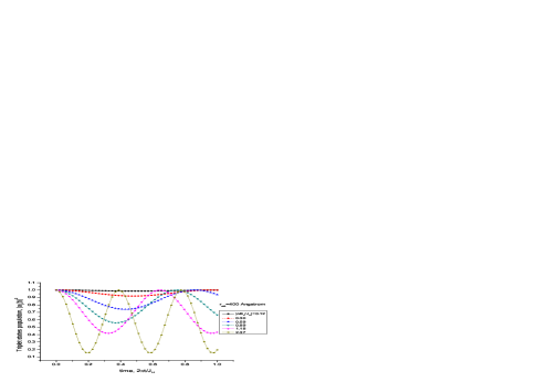
Figure 1: (color online) The triplet states population of electrons in shallow QD centers in GaAs, as a function of time at different magnetic field differences $\Delta B_{z}=0.01,0.025,0.05,0.075,0.1,0.2$T, normalized to the Heisenberg exchange $J_{H}$ constant. Initially the system is in the triplet state $\left|S=1,M_{S}=0\right\rangle$. The distance between QDs is 400 Å.

Clearly, there is an important qualitative difference between pure- and pseudo-spin models. In the former, the singlet-triplet states coupling is a second order effect, while in the latter this coupling is of first order in $H^{st}$ [cf., Eq. (47) and (6)]. Thus, in pure-spin models effects due to $\vec{B}$-field inhomogeneity should be especially (quadratically) small as compared to the corresponding pseudo-spin model effects. In case of negligible $\vec{B}$-field inhomogeneity, as follows from Eq. (45), the pure-spin dynamics is unitary and is governed by the spin Hamiltonian $\mathbf{H}^{tt}$.

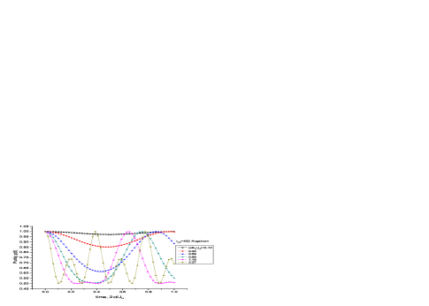
Figure 2: (color online) The purity $\ p(t)=\mathrm{Tr\,}\rho^{2}(t)$ for the same parameters as in Fig. 1.

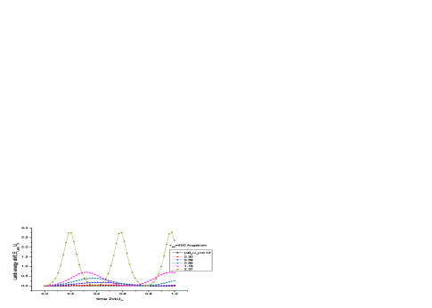
Figure 3: (color online) The Lamb shift energy as a function of time for the same parameters as in Fig. 1.

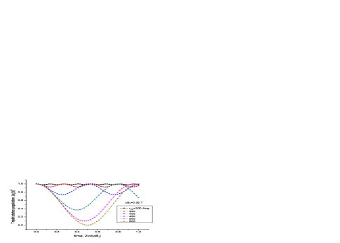
Figure 4: (color online) Triplet states population dependence on interdot separation $r_{AB}=300,$ $\,350,$ $400,$ $\,450,$ $500$, and $600$Å, at a fixed $\Delta B_{z}=0.05$T.

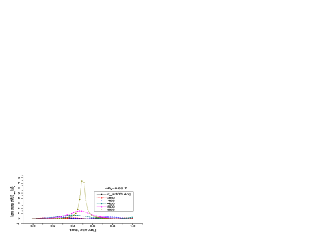
Figure 5: (color online) Lamb energy shift dependence on interdot distance $r_{AB}=300,$ $\,350,$ $400,$ $\,450,$ $500$, and $600$Å, at a fixed $\Delta B_{z}=0.05$T.

Let us now consider a simple numerical example for the non-unitary effects due to the difference field $\Delta\vec{B}$ for an electron localized on a donor impurity in an $n$-doped GaAs semiconductor. To simplify numerics, we assume that $H^{ss}={\rm diag}(\varepsilon_{s1},\varepsilon_{s2},\varepsilon_{s3})$ is diagonal and the singlet-triplet coupling field, $\Delta\vec{B}$, has only a non-zero $z$-component, $\Delta B_{z}$. Then, the corresponding eigenvalue problem, Eq. (21), can be reduced to a biquadratic polynomial equation which could, in principle, be solved exactly. If we neglect the exponentially small coupling field $\delta B_{z}$, proportional to the overlap $S$, the biquadratic equation reduces to a quadratic one and we find for the non-unitary term

$$\mathcal{L}_{t} = \frac{\omega\sin\omega t}{J_{H}^{2}+\frac{1}{2}\Delta B_{z}^{2}(1+\cos\omega t)}\times$$ (51)

$$\left(\left[\mathbf{K},\rho\mathbf{K}^{\dagger}\right]+\left[\mathbf{K}\rho,\mathbf{K}^{\dagger}\right]\right)\quad$$

$$\mathbf{K} = -\frac{i}{4}\Delta B_{z}\cdot J_{asz}$$

and the Lamb shift

$$\mathbf{L}_{t}\mathbf{=}\frac{J_{H}(1-\cos\omega t)}{J_{H}^{2}+\frac{1}{2}\Delta B_{z}^{2}(1+\cos\omega t)}\mathbf{K}^{\dagger}\mathbf{K,}$$ (52)

where $\omega=\sqrt{J_{H}^{2}+\Delta B_{z}^{2}}$. In the limit of small magnetic field inhomogeneity, $|\Delta B_{z}/J_{H}|\ll 1$, $\omega\rightarrow|J_{H}|$ and Eqs. (51) and (52) go over into (47) and (50), respectively. Eq. (52) describes the Lamb energy shift of the triplet state $\left|S=1,M_{S}=0\right\rangle$ due to the coupling between singlet and triplet states induced by the magnetic field inhomogeneity $\Delta B_{z}$. At the magnetic field geometry we have chosen there is no coupling between $\left|S=1,M_{S}=\pm 1\right\rangle$ and $\left|S=1,M_{S}=0\right\rangle$ states.

In Figs. 1-3, we show the results of calculations for the triplet states population, purity, and the Lamb shift energy, respectively, as a function of time at a fixed interdot separation ($r_{AB}=400\,\mathrm{\mathring{A}}$) and different $\Delta B_{z}$. For the Heisenberg interaction constant $J_{H}$ we used an asymptotically correct expression GK03 ; GP63 ; HF64 obtained for hydrogenlike centers in GaAs [note that our $J_{H}=\varepsilon_{t}-\varepsilon_{s}$ is related to the exchange integral $J$ in Ref. GK03, via $J_{H}=-2J$]. Initially, the system is assumed to be in the $\left|S=1,M_{S}=0\right\rangle$ state. As can be seen from Fig. 1, there is a re-distribution between singlet and triplet states population due to the singlet-triplet subspace coupling. At $|\Delta B_{z}/J_{H}|\lesssim 0.1$, the probability of re-distribution is negligible and the time-evolution is basically unitary. With increasing $\Delta B_{z}$, this probability re-distribution is seen to be more pronounced, time-evolution becomes non-unitary (Fig. 2), and $|a_{t}(t)|^{2}$ can drop to the value $J_{H}^{2}/\omega^{2}$ at $t=\pi n/\omega,\,n=1,3,\ldots$. Observe that the non-unitary dynamics reveals repetitions in time and at moments of maximal (minimal) singlet-triplet states probability re-distribution we find maximal (minimal) Lamb energy shifts (Fig. 3). Thus, the non-unitary effects observed are not irreversible and they do not result in a real decoherence process. We do not have in our two-electron model a real, external and infinite “bath”, coupling to which would result in irreversible decoherence effects in the spin system. In Figs. 4,5 we demonstrate the dependence of triplet states population and Lamb energy shifts on the interdot distance $r_{AB}$ at a fixed $\Delta B_{z}=0.05\mathrm{T}$.

III.4 Spin-orbit interaction in pure-spin model

In this subsection we estimate the non-unitary effects in the pure-spin model due to spin-orbit interaction. For simplicity we assume that the external magnetic field is homogeneous and directed along the $z$-axis, with $B_{oz}$ being its $z$-component. Since $\delta\vec{B}_{so}$ is a pure imaginary field (its components are matrix elements between the real states $\tilde{\phi}_{A}$ and $\tilde{\phi}_{B}$ of an odd vector function of the momentum operator, both in vacuum and in the bulk of semiconductors that lack inversion symmetry, Dresselhaus fields,Dres55 as well as in heterostructure zinc-blendes, Rashba fields,BR84 ) we have

$$(\delta B_{so}^{\pm})^{\ast}=-\delta B_{so}^{\mp},\qquad\delta B_{soz}^{\ast}=-\delta B_{soz}.$$ (53)

Using these relationships, the singlet-triplet spin-orbit coupling can be written as

$$H^{st}(\vec{B}_{so})=\left(\begin{array}[]{ccc}0&0&0\\ \frac{1}{2}\delta B_{so}^{+}&-\frac{1}{\sqrt{2}}\delta B_{soz}&-\frac{1}{2}\delta B_{so}^{-}\\ \frac{1}{2}\delta B_{so}^{+}&-\frac{1}{\sqrt{2}}\delta B_{soz}&-\frac{1}{2}\delta B_{so}^{-}\end{array}\right).$$ (54)

The couplings between double-occupancy, singlet and triplet states are seen to be the same. We assume that $H^{ss}={\rm diag}(\varepsilon_{s},\varepsilon_{do},\varepsilon_{do}),$ where $\varepsilon_{s}$ and $\varepsilon_{do}$ are the singlet and double-occupancy states energies, and $H^{tt}={\rm diag}(\varepsilon_{t+},\varepsilon_{t},\varepsilon_{t-})$, where $\varepsilon_{t}$ is a triplet state energy and $\varepsilon_{t\pm}=\varepsilon_{t}\pm B_{0z}$. Within these approximations, the 6-by-6 eigenvalue problem Eq. (21) is then reduced to computing the roots of the biquadratic equation AS64

$$E^{4}+a_{3}E^{3}+a_{2}E^{2}+a_{1}E+a_{0}=0$$ (55)

where

$$a_{3} = -\sum\limits_{i=1}^{4}\varepsilon_{i},\qquad a_{2}=\sum\limits_{i\neq j}\varepsilon_{i}\varepsilon_{j}-\sum\limits_{\alpha=x,y,z}|\delta B_{so\alpha}|^{2},$$

$$a_{1} = -\sum\limits_{i\neq j\neq k}\varepsilon_{i}\varepsilon_{j}\varepsilon_{k}+$$

$$\left(|\delta B_{soz}|^{2}+\frac{1}{2}[|\delta B_{sox}|^{2}+|\delta B_{soy}|^{2}]\right)(\varepsilon_{2}+\varepsilon_{4})+$$

$$(|\delta B_{sox}|^{2}+|\delta B_{soy}|^{2})\varepsilon_{3},$$

$$a_{0} = \prod\limits_{i=1}^{4}\varepsilon_{i}-|\delta B_{soz}|^{2}\varepsilon_{2}\varepsilon_{4}-$$

$$\frac{1}{2}[|\delta B_{sox}|^{2}+|\delta B_{soy}|^{2}]\varepsilon_{3}(\varepsilon_{2}+\varepsilon_{4}),$$

$$\varepsilon_{1} = \varepsilon_{s},\qquad\varepsilon_{2}=\varepsilon_{t+},\qquad\varepsilon_{3}=\varepsilon_{t},\qquad\varepsilon_{4}=\varepsilon_{t-}.$$

For hydrogenlike centers one can estimate the energies $\varepsilon_{do}$ and $\varepsilon_{t}$ as follows. The ground energy of two well separated hydrogen atoms is $E_{2\mathrm{H}}\approx-27.2\,\mathrm{eV}$ . Using for GaAs the scaling factor $K_{\mathrm{GaAs}}=m^{\ast}/\varepsilon^{2}\approx 4.6\cdot 10^{-4}$ one can estimate $\varepsilon_{t}\approx K_{\mathrm{GaAs}}E_{2\mathrm{H}}=-12.6\,\mathrm{meV}$. $\varepsilon_{do}$ is located higher than $\varepsilon_{t}$ due to mainly interelectron repulsion $\tilde{v}_{\mathrm{ee}}(AA;AA)$ so that $\varepsilon_{do}-\varepsilon_{t}=\tilde{v}_{\mathrm{ee}}(AA;AA)\approx 12.6\,\mathrm{meV}$.

If $\delta B_{so\alpha}\equiv 0,$ $\alpha=x,y,z$, the roots of Eq. (55) $E_{i}$ are equal to $\varepsilon_{i}$, $i=1,\ldots,4$. The two other roots are $E_{5}=\varepsilon_{do}$ and $E_{6}=\varepsilon_{s}$. The corresponding eigenvectors are

$$\left|e_{k}\right\rangle = d_{k}\left(0,1,1,-\frac{\delta B_{so}^{-}}{E_{k}-\varepsilon_{2}},\frac{\sqrt{2}\delta B_{soz}}{E_{k}-\varepsilon_{3}},\frac{\delta B_{so}^{+}}{E_{k}-\varepsilon_{4}}\right)^{T},\qquad$$

$$k = 1,\ldots,4,$$

$$\left|e_{5}\right\rangle = \frac{1}{\sqrt{2}}\left(0,1,-1,0,0,0\right)^{T},\qquad$$

$$\left|e_{6}\right\rangle = \left(1,0,0,0,0,0\right)^{T},$$ (56)

where

$$d_{k} = \left(2+[|\delta B_{sox}|^{2}+|\delta B_{soy}|^{2}]\right.\times$$

$$\left.\left(\frac{1}{(E_{k}-\varepsilon_{2})^{2}}+\frac{1}{(E_{k}-\varepsilon_{4})^{2}}\right)+\frac{2|\delta B_{soz}|^{2}}{(E_{k}-\varepsilon_{3})^{2}}\right)^{-1/2}.$$

Notice that the above formulas are not valid in the degenerate case: $B_{0z}=0$ and $\varepsilon_{2}=\varepsilon_{3}=\varepsilon_{4}=\varepsilon_{t}$. In this case the biquadratic Eq. (55) reduces to two quadratic ones, two roots of which are degenerate, $E_{1}=E_{2}=\varepsilon_{t}$. Formally, one gets singularities in Eq. (56) at $E_{1}=E_{2}=\varepsilon_{t}$. Therefore, the simpler, degenerate case should be analyzed separately and the corresponding formulas [not shown here] can be derived.

Let us now find the spin-orbit field

$$\begin{array}[]{lll}\delta\vec{B}_{so}&=&\left\langle\tilde{\phi}_{A}\right|\vec{B}_{so}(\vec{p})\left|\tilde{\phi}_{B}\right\rangle\approx\left\langle\phi_{A}\right|\vec{B}_{so}(\vec{p})\left|\phi_{B}\right\rangle\\ &=&\int d\vec{r}\,\phi_{A}(|\vec{r}-\vec{R}|)\vec{B}_{so}(-i\nabla_{\vec{r}})\phi_{B}(r)\\ &=&\vec{B}_{so}(-i\nabla_{\vec{R}})\int d\vec{r}\,\phi_{A}(|\vec{r}-\vec{R}|)\phi_{B}(r)\\ &=&\vec{B}_{so}(-i\nabla_{\vec{R}})S(R)\end{array}$$ (57)

where $\vec{B}_{so}(\vec{p})$ is an odd function of the momentum operator $\vec{p}=-i\nabla_{\vec{r}}$ and $\vec{R}=\vec{r}_{AB}$. In particular, in zinc-blende semiconductors such as GaAs, $\vec{B}_{so}$ is cubic in the components of $\vec{p}$: Dres55 ; DP71

$$B_{so\alpha} = A_{so}p_{\alpha}(p_{\beta}^{2}-p_{\gamma}^{2}),\qquad$$

$$\alpha,\beta,\gamma = \{\mathrm{cyclic\,permutations\,of\quad}x,y,z\}$$

$$A_{so} = \alpha_{so}\left(m^{\ast}\sqrt{2m^{\ast}E_{g}}\right)^{-1},$$ (58)

where $m^{\ast}$ is the effective mass of the electron, $E_{g}$ is the band gap [$m^{\ast}\approx 0.072,$ $E_{g}\approx 1.43\,\mathrm{eV}$ for GaAs], $p_{x}$, $p_{y}$, $p_{z}$ are components of the momentum along the cubic axes $[100]$, $[010]$, and $[001]$ respectively. The dimensionless coefficient $\alpha_{so}=0.07$ for GaAs. From Eqs. (57) and (58) we obtain

$$B_{so\alpha} = iA_{so}\frac{R_{\alpha}(R_{\beta}^{2}-R_{\gamma}^{2})}{R^{3}}\left\{S^{{}^{\prime\prime\prime}}(R)-\right.$$ (59)

$$\left.\frac{3}{R}S^{{}^{\prime\prime}}(R)+\frac{3}{R^{2}}S^{{}^{\prime}}(R)\right\}$$

The overlap integral Sla63 $S(r=R/a_{B})=(1+r+r^{2}/3)\exp(-r)$ for hydrogenlike centers [$a_{B}\approx 92\,\mathrm{\mathring{A}}$ for GaAs] and Eq. (59) reduces to

$$B_{sox} = i(0.83\,\mathrm{meV})\sin\theta\cos\varphi(\sin^{2}\theta\sin^{2}\varphi-\cos^{2}\theta)\times$$ (60)

$$\left(-\frac{1}{3}\right)r^{2}\exp(-r)$$

where $(R,\theta,\varphi)$ are spherical coordinates of the vector $\vec{R}$, with other components being obtained by cyclic interchange of indices.

Figure 6: (color online) Triplet states population dependence on spin-orbit interaction as a function of time, at different interdot separations $r_{AB}$ and fixed orientation of the interdot radius-vector, $\vec{r}_{AB}$, ($\theta=\pi/4,\varphi=\pi/3$) [see text]. The initial triplet states population is taken to be equal. The external magnetic field $B_{0z}=0.5$T.

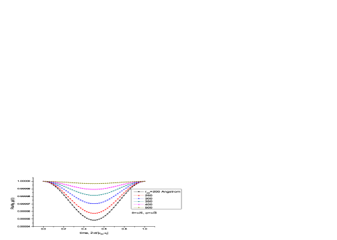
Figure 7: (color online) The purity in the presence of spin-orbit coupling. All parameters are the same as in Fig. 6.

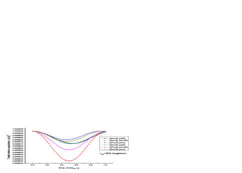
Figure 8: (color online) Effect of spin-orbit angular anisotropy on triplet states population. All parameters are the same as in Fig. 6.

In Figs. 6 and 7 we display the time-dependence of the triplet states population and the purity, which is induced by the spin-orbit interaction, Eq. (60), at a fixed orientation, ($\theta=\pi/4,\varphi=\pi/3$), and different $r_{AB}$ in the range 200-500Å. Observe that the maximal re-distribution of singlet-triplet probability occurs at $2\pi t/|\varepsilon_{do}-\varepsilon_{t}|=0.5$ and the spin-orbit interaction effect diminishes as $r_{AB}$ increases. The maximal singlet-state probability achieved at $r_{AB}=200$ $\mathrm{\mathring{A}}$ is seen to be quite small, $\sim 10^{-5}$. As compared to the non-unitary effects induced by $\vec{B}$-field inhomogeneity, the spin-orbit effects are on average four orders of magnitude smaller. The angular dependence of the population of triplet states on the interdot radius-vector orientation at a fixed $r_{AB}=200\,\mathrm{\mathring{A}}$ is illustrated in Fig. 8.

III.5 The $\vec{B}$-field interaction in the pseudo-spin model

Using Eqs. (42) and (45), the effective Hamiltonian matrix Eq. (6) in the basis $\left\{\Phi_{s1},\Phi_{ti},i=1,2,3\right\}$ can be rewritten as

$$\mathcal{H}_{\mathrm{eff}}=\left(\begin{array}[]{cccc}\varepsilon_{s}&\frac{1}{2\sqrt{2}}\Delta B^{+}&-\frac{1}{2}\Delta B_{z}&-\frac{1}{2\sqrt{2}}\Delta B^{-}\\ \frac{1}{2\sqrt{2}}\Delta B^{-}&\varepsilon_{t}+B_{avz}&B_{av}^{-}&0\\ -\frac{1}{2}\Delta B_{z}&B_{av}^{+}&\varepsilon_{t}&B_{av}^{-}\\ -\frac{1}{2\sqrt{2}}\Delta B^{+}&0&B_{av}^{+}&\varepsilon_{t}-B_{avz}\end{array}\right)$$ (61)

where for simplicity we neglected contributions from the double-occupancy states [the resolvent term in Eq. (3)]. Alternatively, in the pseudo-spin representation we get

$$\mathcal{H}_{\mathrm{eff}} = \left(\frac{1}{4}\varepsilon_{s}+\frac{3}{4}\varepsilon_{s}\right)I+J_{H}\,\vec{s}_{A}\cdot\vec{s}_{B}+$$ (62)

$$\vec{B}_{av}\cdot(\,\vec{s}_{A}+\vec{s}_{B})+\frac{\Delta\vec{B}}{2}\cdot(\,\vec{s}_{A}-\vec{s}_{B})$$

$$= \left(\frac{1}{4}\varepsilon_{s}+\frac{3}{4}\varepsilon_{t}\right)I+J_{H}\,\vec{s}_{A}\cdot\vec{s}_{B}+$$

$$\vec{B}_{A}\cdot\vec{s}_{A}+\vec{B}_{B}\cdot\vec{s}_{A},$$

where $\vec{B}_{A}=\vec{B}_{av}+\Delta\vec{B}/2$ and $\vec{B}_{B}=\vec{B}_{av}-\Delta\vec{B}/2$ are the local magnetic fields at sites $A$ and $B$, respectively. The term $J_{H}\,\vec{s}_{A}\cdot\vec{s}_{B}$ is the familiar Heisenberg interaction. In matrix form, Eq. (62) can be rewritten as

$$\mathcal{H}_{\mathrm{eff}} = \left(\begin{array}[]{cccc}\varepsilon_{1}&\frac{1}{2}B_{A}^{-}&0&0\\ B_{A}^{+}&\varepsilon_{2}&\frac{1}{2}J_{H}&0\\ 0&\frac{1}{2}J_{H}&\varepsilon_{3}&\frac{1}{2}B_{B}^{-}\\ 0&0&\frac{1}{2}B_{B}^{+}&\varepsilon_{4}\end{array}\right)$$ (67)

$$\varepsilon_{1} = \varepsilon_{t}+\frac{1}{2}B_{Az},\quad\varepsilon_{2}=\varepsilon_{t}-\frac{1}{2}(J_{H}+B_{Az}),$$

$$\varepsilon_{3} = \varepsilon_{t}-\frac{1}{2}(J_{H}-B_{Bz}),\quad\varepsilon_{4}=\varepsilon_{t}-\frac{1}{2}B_{Bz}$$

where $B_{A,B}^{\pm}=B_{A,Bx}\pm iB_{A,By}$.

The Hamiltonian Eq. (61) generates a unitary evolution

$$U_{\mathrm{eff}}(t)=\exp(-it\mathcal{H}_{\mathrm{eff}})$$ (68)

in $\mathbb{C}^{4}$. At a fixed set of parameters $\varepsilon_{s},\varepsilon_{t},\vec{B}_{A},\vec{B}_{B}$ the propagator $U_{\mathrm{eff}}(t)$ does not provide a universal set of unitary gates in $\mathbb{C}^{4}$. Any unitary transformation $U\in U(4)$ can be represented as a product of a phase factor $\exp(i\alpha)$, where $\alpha$ is a real parameter, and a unitary transformation $U_{S}\in SU(4)$. Any transformation $U_{S}$  is determined by $M=4^{2}-1=15$ independent real parameters $(\theta_{1},\ldots,\theta_{15})$ so that

$$U_{S}(\theta_{1},\ldots,\theta_{M})=\exp\left(-i\sum\limits_{i=1}^{M}\theta_{i}F_{i}\right),$$ (69)

where the set of generators $\{F_{i}\}$ is an orthonormalized traceless, Hermitian matrix set that forms a Lie algebra $su(4)$ [$F_{i}$’s form a complete basis in a real $M$-dimensional vector space; they are analogs of Pauli matrices, $\sigma_{\alpha}$, $\alpha=x,y,z$, in $su(2)$ - see, e.g., Ref. AL87, ]. From the representation Eq. (69) it follows immediately that $U_{\mathrm{eff},S}(t)=\exp\left(-it\left(\frac{1}{4}\varepsilon_{s}+\frac{3}{4}\varepsilon_{t}\right)\right)U_{\mathrm{eff}}(t)$ cannot match an arbitrary $U_{S}$, because the number of independent parameters in Eq. (61) is at most $8$ – fewer than the number of $\theta_{i}$’s. This can also be understood from the fact that the form of the Hamiltonian matrix, Eq. (61), is not generic. In particular, the matrix is sparse, i.e., the entries $(2,4)$ and $(4,2)$ are zeros.

However, compositions of unitary transformations Eq. (68) taken at different sets of parameters can provide a universal set of unitary gates in $\mathbb{C}^{4}$. A well-known example of universal gates is provided by the Heisenberg interaction (at $J_{H}\neq 0$) with single-spin addressing (at $\Delta\vec{B}\neq 0$).Loss:98

From Eq. (61) it follows that a necessary and sufficient condition for obtaining a universal set of gates on two spins is to have an inhomogeneity in the magnetic field $\Delta\vec{B}\neq 0$ [the source of inhomogeneity can be different, it can be either strongly localized magnetic fields or $g$-factor engineering] and the Heisenberg interaction, $J_{H}\neq 0$. The reason is that when $\Delta\vec{B}=0$, the Hamiltonian Eq. (61) and the corresponding unitary transformations take a block-diagonal form, with singlet-triplet entries being zeros, while when $J_{H}=0$,  the Hamiltonian form (67) will have zero off-diagonal block-matrices. Clearly, even a composition of such unitary transformations taken at different sets of parameters, either $\varepsilon_{s},\varepsilon_{t},\vec{B}_{A}=\vec{B}_{B}$ or $\varepsilon_{s}=\varepsilon_{t},\vec{B}_{A},\vec{B}_{B}$, will be in a block-diagonal form and it cannot reproduce an arbitrary unitary transformation. Note that when one allows for encoding a qubit into three or more spins, the Heisenberg interaction alone is universal in the pseudo-spin model,Bacon:99a ; Kempe:00 and Heisenberg along with an inhomogneous magnetic field is universal for an encoding of a single qubit into pair of spins.LidarWu:01

Moreover, it should be noted that in the homogeneous magnetic field case unitary transformations restricted to the triplet subspace will not provide a universal set of gates. To prove this statement, let us consider a composition of two unitary transformations in the triplet subspace:

$$\begin{array}[]{l}\exp(-it_{1}H^{tt}(\vec{B}_{1}))\exp(-it_{2}H^{tt}(\vec{B}_{2}))=\\ \exp(-i(t_{1}+t_{2})H_{\mathrm{eff}}^{tt})=\\ \exp\left(-i(t_{1}+t_{2})\varepsilon_{t}-it_{1}H^{tt}(\vec{B}_{1})-it_{2}H^{tt}(\vec{B}_{2})-\right.\\ \left.\frac{t_{1}t_{2}}{2}\left[H^{tt}(\vec{B}_{1}),H^{tt}(\vec{B}_{2})\right]+\cdots\right),\end{array}$$ (70)

where on the right-hand-side we used the Campbell-Hausdorff formula.Cor90 From Eq. (42) one obtains

$$\left[H^{tt}(\vec{B}_{1}),H^{tt}(\vec{B}_{2})\right]=i\left(\begin{array}[]{ccc}2\mathcal{B}_{z}&\mathcal{B}^{-}&0\\ \mathcal{B}^{+}&0&\mathcal{B}^{-}\\ 0&\mathcal{B}^{+}&-2\mathcal{B}_{z}\end{array}\right),$$ (71)

where $\mathcal{\vec{B}=}[\vec{B}_{1}\times\vec{B}_{2}]$ and $\mathcal{B}^{\pm}=\mathcal{\vec{B}}_{x}\pm i\mathcal{\vec{B}}_{y}$. Since the higher-order terms in the Campbell-Hausdorff formula consist of nested commutators between $H^{tt}(\vec{B}_{1})$ and $H^{tt}(\vec{B}_{2})$, we find that the effective Hamiltonian $H_{\mathrm{eff}}^{tt}$ corresponding to the product of two unitary transformations will still have a sparse form, with the $(1,3)$ and $(3,1)$ entries being zeros.

III.6 Is it possible to obtain a universal set of gates in the pure-spin model?

Simultaneously, we have just proved that in the pure-spin model, in the case of a homogeneous magnetic field, unitary transformations in the triplet subspace will not provide a universal set of gates. On the other hand, at $\Delta\vec{B}\neq 0$, we have already shown that the evolution of the spin-density matrix is non-unitary. Let us assume that we have a non-unitary gate $\mathcal{L}_{1}$ so that $\rho(t_{1})=\mathcal{L}_{1}(t_{1})\rho(0)$. How could one define a composition of two non-unitary gates, $\mathcal{L}_{2}\mathcal{L}_{1}$? In order to do this unambiguously, $\mathcal{L}_{2}$ should obey a compatibility condition with the initial state [because a non-unitary $\mathcal{L}$-gate is not totally independent of the initial state, it includes some sort of correlation information encoded in the initial state], that is a correlation $R_{m}(t_{1})$ established between $a_{s}(t_{1})$ and $a_{t}(t_{1})$ amplitudes at $t=t_{1}$ should be included in in the definition of the corresponding dynamics generator operators in $\mathcal{L}_{2}$. Eq. (19), where the left-hand-side and $H^{ts}$ should be replaced by $R_{m}(t_{1})$ and the identity matrix, respectively, provides a relationship between $R_{m}(t_{1})$ and $R_{m}(0)$. If the correlation between the amplitudes at $t=0$ and $t=t_{1}$ is the same, $R_{m}(t_{1})=$ $R_{m}(0)$, then we obviously have $\mathcal{L}_{1}=\mathcal{L}_{2}=\mathcal{L}$ and $\mathcal{L}_{2}(t_{2})\mathcal{L}_{1}(t_{1})=\mathcal{L(}t_{1}+t_{2})$.

In the total Hilbert space, the state is defined by 11 real parameters. While in the reduced description, the spin-density matrix is defined by 5 real parameters (for more on the spin density matrix parametrization in terms of $a$’s, see Section V). Fixing a correlation in the initial state, $a_{s}(0)=R_{m}(0)a_{t}(0)$, we have 3 complex equations between the amplitudes $a_{s}(0)$ and $a_{t}(0)$, which define a 5D real manifold embedded into the total Hilbert space. Using these equations we can separate 6 extra real degrees of freedom that we have in the total state description from those in the spin-density matrix description. However, these extra degrees of freedom are not eliminated in the spin-density description, they are included in the form of correlation matrix $R_{\alpha}(0)$, $\alpha=\{s,t,m\}$. It was shown in part I that Eq. (14) provides an exact description of quantum evolution, in the spin-density space. Therefore, as long as we have a universal set of unitary gates in the total Hilbert space, this set of gates will be translated into the corresponding universal set of non-unitary gates generated by Eq. (14) because no information is lost in our “reduced” spin-density matrix description.

III.7 Spin-orbit interaction in the pseudo-spin model

Let us consider spin-orbit effects, which are proportional to $\delta B_{so}$, in the pseudo-spin model. From Eq. (6) we obtain

$$\mathcal{H}_{so}(\delta\vec{B}_{so})=\sum_{kk^{\prime}=2,3}H_{1k}^{ss}\left(\frac{1}{\bar{E}I-H^{ss}}\right)_{kk^{\prime}}^{-1}F_{k^{\prime}}(\delta\vec{B}_{so}),$$ (72)

where

$$F_{k}(\delta\vec{B}_{so})=\sum_{i=1}^{3}\left(H_{ki}^{st}(\delta\vec{B}_{so})\mathbf{K}_{i}+(H_{ki}^{st}(\delta\vec{B}_{so}))^{\ast}\mathbf{K}_{i}^{\dagger}\right)$$ (73)

It follows from Eq. (54) that $H_{2i}^{st}=H_{3i}^{st}$, $F_{2}=F_{3}$ and Eq. (73) can be reduced to

$$F_{2,3}(\delta\vec{B}_{so})=F(\delta\vec{B}_{so})=i\sqrt{2}\delta\vec{B}_{so}\left[\vec{s}_{A}\times\vec{s}_{B}\right]$$ (74)

Then, Eq. (72) can be rewritten as

$$\mathcal{H}_{so}(\delta\vec{B}_{so})=\mathcal{A}_{do}F(\delta\vec{B}_{so})$$ (75)

where the coefficient $\mathcal{A}_{do}$ is proportional to the ratios of the amplitudes of double occupancy transitions ($H_{12}^{ss}$ and $H_{13}^{ss}$) and the energies of interelectron interaction ($H_{22}^{ss}-\bar{E}$ and $H_{33}^{ss}-\bar{E}$) in doubly occupied QDs:

$$\mathcal{A}_{do} = \sum_{kk^{\prime}=2,3}H_{1k}^{ss}\left(\frac{1}{\bar{E}I-H^{ss}}\right)_{kk^{\prime}}$$ (76)

$$= \frac{1}{\Delta}\left[H_{12}^{ss}(\bar{E}-H_{33}^{ss}-H_{32}^{ss})+\right.$$

$$\left.H_{12}^{ss}(\bar{E}-H_{22}^{ss}-H_{23}^{ss})\right]$$

$$\approx \frac{H_{12}^{ss}}{\bar{E}-H_{22}^{ss}}+\frac{H_{13}^{ss}}{\bar{E}-H_{33}^{ss}}.$$

Here, the determinant is

$$\Delta=(\bar{E}-H_{22}^{ss})(\bar{E}-H_{33}^{ss})-|H_{23}^{ss}|^{2}.$$ (77)

The effective spin-orbit interaction Hamiltonian Eq. (75) is different from the corresponding one obtained by Kavokin.Kav01 In our derivation the double-occupancy states are essential, whereas in Ref. Kav01, these states are totally neglected. We showed above that neglecting double-occupancy states results in zero spin-orbit coupling. The very physical picture put forward in Ref. Kav01, to support the derivation was based on the assumption that when one of the two electrons localized at centers $A$ or $B$ tunnels to the adjacent center (say, from $A$ to $B$), it experiences the influence of the spin-orbit field resulting from the under-barrier motion of the electron. Neglecting double occupancy states means that the second electron should simultaneously tunnel from $B$ to $A$ so that the two electrons can never be found in the same QD. Indeed, in Ref. Kav01, this simultaneous two-electron transition is described by the product of two matrix elements: the overlap $S$ and $(\delta\vec{B}_{so})_{\alpha}$, $\alpha=x,y,z$ [$\mathcal{H}_{so}\sim S(\delta\vec{B}_{so}\cdot\left[\vec{s}_{A}\times\vec{s}_{B}\right])$, our $\delta\vec{B}_{so}$ is related to Kavokin’s $\mathbf{b}$-field via $\delta\vec{B}_{so}=-i\mathbf{b}$, and the overlap via $S=\Omega$]. With the orthogonalized molecular-type, two-center orbitals such a one step two-electron transition gives a zero contribution since the spin-orbit interaction is a one-electron operator and the overlap $\tilde{S}=\left\langle\tilde{\phi}_{A}\right|\left.\tilde{\phi}_{B}\right\rangle=0$. Eq. (72) describes the two-step mechanism: in the first step, the two-electron system makes a transition from the singly-occupied state $\Phi_{s1}$ to the intermediate, double-occupancy states $\Phi_{s2}$, $\Phi_{s3}$ due to the inter-electron interaction ($H_{1k}^{ss},$ $k=1,2$ terms). Then in the second step, as a result of the spin-orbit interaction, the system makes transitions from $\Phi_{s2}$, $\Phi_{s3}$ to $\Phi_{ti}$ triplet states (the $H_{ki}^{st}$ terms).

Let us find an estimate for

$$\mathcal{A}_{do}(R) \approx -\frac{2\sqrt{2}}{|\varepsilon_{do}-\varepsilon_{t}|}\iint d\vec{r}_{1}d\vec{r}_{2}\,\phi^{2}(r_{1})\times$$ (78)

$$\phi(|\vec{r}_{2}-\vec{R}|)\frac{1}{\varepsilon|\vec{r}_{2}-\vec{r}_{1}|}\phi(r_{2}),$$

where the hydrogenlike orbital $\phi(r)=(\pi a_{B}^{3})^{-1/2}\exp(-r/a_{B})$. Since electron 1 in Eq. (78) is localized around the effective Bohr radius $a_{B}$, one can approximate

$$\frac{1}{|\vec{r}_{2}-\vec{r}_{1}|}\approx\frac{1}{|\vec{r}_{2}-a_{B}\vec{r}_{1}/r_{1}|}.$$ (79)

Then, the remaining integrals can be calculated exactly and we obtain

$$\begin{array}[]{ccc}\mathcal{A}_{do}(r=R/a_{B})&\approx&-\frac{4\sqrt{2}}{er}\left\{4eF_{1}(r)\right.-\\ &&2\left[F_{1}(r+1)+F_{1}(r-1)\right]-\\ &&\left[F_{2}(r+1)-F_{2}(r-1)\right]+\\ &&\left.2\left[F_{0}(r+1)-F_{0}(r-1)\right]\right\}\end{array}$$ (80)

where

$$\begin{array}[]{lll}F_{0}(x)&=&\frac{{\rm sign}(x)}{48}\left[15(1+|x|)+6|x|^{2}+|x|^{3}\right]\exp(-|x|),\\ F_{1}(x)&=&\frac{1}{48}\left[3|x|(1+|x|)+|x|^{3}\right]\exp(-|x|),\\ F_{2}(x)&=&\frac{{\rm sign}(x)}{2}(1+|x|)\exp(-|x|).\end{array}$$ (81)

Here, we used the same estimate for $\varepsilon_{do}-\varepsilon_{t}$ as in Section III.4.

Figure 9: Spin-orbit interaction reduction coefficient Eq. (82) as a function of interdot distance for GaAs.

In order to compare our calculations to Kavokin’s result for GaAs, we have plotted in Fig. 9 the spin-orbit interaction reduction coefficient

$$K_{so}=\frac{|\mathcal{A}_{do}|}{\sqrt{2}S},$$ (82)

which is exactly the ratio of our and Kavokin’s estimates, as a function of interdot distance. As one can see, $K_{so}$ decreases from 0.98 to 0.46 in the range $r_{AB}\sim 300-700\mathrm{\mathring{A}}$. Interestingly, our results qualitatively agree with the results of Ref. GK03, , which obtained in the region of interest [$r_{AB}\sim(3-7)a_{B}$] a reduction of about one-half relative to that of Refs. Kav01, ; DK02, . According to Ref. GK03, , $\mathcal{H}_{so}\sim 2J\gamma_{\mathrm{GK}}$, where $J$ is the exchange integral calculated using the medium hyperplane method GP63 ; HF64 and $\gamma_{\mathrm{GK}}$ is an angle of spin rotation due to spin-orbit interaction introduced by Gor’kov and Krotkov [$\gamma_{\mathrm{GK}}\approx\frac{1}{2}\gamma_{\mathrm{K}}$, $\gamma_{\mathrm{K}}$ being the corresponding angle of spin rotation introduced by Kavokin]. Note that Kavokin’s $\gamma_{\mathrm{K}}$ and $J$ are not independent parameters. In Ref. Kav01, , $\gamma_{\mathrm{K}}$ was defined as $\Omega b/J$ so that their product $2J\gamma_{\mathrm{K}}=2\Omega b$ does not depend explicitly on $J$.

IV Electrons on Liquid Helium

Recently, Lyon suggested that the spin of electrons floating on the surface of liquid helium (LHe) will make an excellent qubit.Lyon06 Lyon’s proposal, instead of using the spatial part of the electron wavefunction as a qubit as in the charge-based proposal,PD99 ; DP00 ; DPS03 ; DPS04 takes advantage of the smaller vulnerability of the electron’s spin to external magnetic perturbations and, as a consequence, a longer spin-coherence time. It also has the important advantage over semiconductor spin-based proposals (as first pointed out in the charge-based proposalPD99 ; DP00 ; DPS03 ; DPS04 ) that, with the electrons residing in the vacuum, several important sources of spin decoherence are eliminated so that the environment effects are highly suppressed (the spin-coherence time is estimatedLyon06 to be $T_{2}>100$s).

The geometry of the system with the electrons trapped at the LHe-vacuum interface (see Fig. 2 in Ref. Lyon06, ), is conceptually similar to that of semiconductor heterostructures. The two electrons are trapped at sites $\vec{r}_{A}$ and $\vec{r}_{B}$ ($\vec{r}_{A,B}$ are radius-vectors of the centers of quantum dots in the $z=0$ plane) by the two attractive centers created by two charged spherical electrodes located below the LHe surface at distance $h$ and separated by the interdot distance $r_{AB}=|\vec{r}_{A}-\vec{r}_{B}|$:

$$V_{\rm tr}(z,\vec{r}) = -\frac{\Lambda}{z}+V_{A}(z,\vec{r})+V_{B}(z,\vec{r})$$ (83)

$$V_{A,B}(z,\vec{r}) = -\frac{Q_{A,B}}{\sqrt{\left(z+h\right)^{2}+\left(\vec{r}-\vec{r}_{A,B}\right)^{2}}},$$ (84)

where the first potential, $-\Lambda/z$, is due to attraction to the image charge induced by an electron in the LHe [$\Lambda=(\varepsilon-1)/(4(\varepsilon+1))\approx 7\cdot 10^{-3}$, with $\varepsilon\approx 1.057$ being the dielectric constant of helium]. For purposes of interaction control, the $Q_{A,B}$ charges on the electrodes can be made variable in time. The electrons are prevented from penetrating into helium by a high potential barrier ($\sim 1$ eV) at the helium surface, so that formally one can put $V_{\rm tr}=\infty$ at $z<0$. The in-plane and out-of-plane motion of electrons in the potential of Eq. (83) is in general non-separable. However, near the electrode’s position $\vec{r}_{A,B}$ the potential of Eq. (84) is approximately separable in the $z$ and $\vec{r}$ coordinates

$$V_{A,B}(z,\vec{r})\approx-\frac{Q_{A,B}}{h}+\mathcal{E}_{\perp A,B}\,z+\frac{1}{2}\omega_{A,B}^{2}\left(\vec{r}-\vec{r}_{A,B}\right)^{2},$$ (85)

where it is assumed that $z$ and $|\vec{r}-\vec{r}_{A,B}|\ll h$ and $\mathcal{E}_{\perp A,B}=Q_{A,B}/h^{2}$, $\omega_{A,B}=\left(Q_{A,B}/h^{3}\right)^{1/2}$. In the separable approximation of Eq. (85), the electron’s motion in the $z$-direction [$z>0$] is described by a 1D-Coulomb potential perturbed by a small Stark interaction and the in-plane motion by a 2D-oscillatory potential. We assume that the out-of-plane motion in the $z$-direction is “frozen” in the ground state of a 1D-Coulomb potential

$$\varphi_{0}^{C}(z)=2\sqrt{\Lambda}(\Lambda z)\exp(-\Lambda z),$$ (86)

and the in-plane motion, in a superposition of the in-plane confining oscillatory potential and, possibly, a perpendicular magnetic field, is described by the Fock-Darwin (FD) states of Eq. (25). Then, the calculation of $h_{ij}$ and $v_{ee}(ij;kl)$ in Eqs. (29)-(31) in the chosen basis set is reduced to the one-dimensional integrals

$$h_{AB} = \left[-\frac{\Lambda}{2}+\frac{1}{4l_{A}^{2}}-2\Lambda Q_{A}g_{c}(\alpha,\beta,\lambda_{A})-\right.$$

$$\left.2\Lambda Q_{B}g_{c}(\alpha,\beta,\lambda_{B})\right]S_{AB},$$

$$h_{AA} = -\frac{\Lambda}{2}+\frac{1}{4l_{A}^{2}}-2\Lambda Q_{A}g_{c}(\alpha,\beta_{A},0)-$$

$$2\Lambda Q_{B}g_{c}(\alpha,\beta_{A},2\Lambda r_{AB}),$$

$$h_{BB} = -\frac{\Lambda}{2}+\frac{1}{4l_{B}^{2}}-2\Lambda Q_{A}g_{c}(\alpha,\beta_{B},2\Lambda r_{AB})-$$

$$2\Lambda Q_{B}g_{c}(\alpha,\beta_{B},0),$$

$$g_{c}(\alpha,\beta,\lambda) = \int_{0}^{\infty}dx\,J_{0}(\lambda x)\times$$ (87)

$$\exp\left(-\alpha x-\beta x^{2}\right)/(x+1)^{3},$$

$$\alpha = 2\Lambda h,\quad\beta=\frac{\left(2\Lambda l_{A}l_{B}\right)^{2}}{l_{A}^{2}+l_{B}^{2}},\quad$$

$$\beta_{A,B} = 2(\Lambda l_{A,B})^{2},\quad\lambda_{A,B}=\frac{2\Lambda l_{B,A}^{2}}{l_{A}^{2}+l_{B}^{2}}r_{AB},$$

$$v_{ee}(AB;CD) = N_{ee}g_{ee}(a,b),$$

$$N_{ee} = \frac{\Lambda l_{A}l_{B}l_{C}l_{D}}{(l_{A}^{2}+l_{C}^{2})(l_{B}^{2}+l_{D}^{2})}\times$$

$$\exp\left(-\frac{r_{AC}^{2}}{4(l_{A}^{2}+l_{C}^{2})}-\frac{r_{BD}^{2}}{4(l_{B}^{2}+l_{D}^{2})}\right),$$

$$g_{ee}(a,b) = \int_{0}^{\infty}dx\,J_{0}(bx)\times$$ (88)

$$(3x^{2}+9x+8)(x+1)^{-3},$$

$$a = 4\Lambda^{2}\left(\frac{l_{A}^{2}l_{C}^{2}}{l_{A}^{2}+l_{C}^{2}}+\frac{l_{B}^{2}l_{D}^{2}}{l_{B}^{2}+l_{D}^{2}}\right),\quad$$

$$b = 2\Lambda\left|\frac{l_{C}^{2}\vec{r}_{A}+l_{A}^{2}\vec{r}_{C}}{l_{A}^{2}+l_{C}^{2}}-\frac{l_{D}^{2}\vec{r}_{B}+l_{B}^{2}\vec{r}_{D}}{l_{B}^{2}+l_{D}^{2}}\right|,$$

where $i=A,B,C,D$ in the two-electron matrix elements denotes orbitals with the effective lengths $l_{i}$ localized at $\vec{r}_{i}$, and $J_{0}(x)$ is the zeroth order Bessel function. From Eq. (88) one can obtain the following expression for the Heisenberg interaction constant

$$J_{H} = -1.36\cdot 10^{4}\Lambda g_{ee}(a,0)S^{2}\text{{\ meV}}$$ (89)

$$a = \frac{8\Lambda^{2}l_{A}^{2}l_{B}^{2}}{l_{A}^{2}+l_{B}^{2}}.$$

Note that $J_{H}$ is proportional to the square of the overlap matrix element $S$, Eq. (27), and the integral $g_{ee}(a,0)$ does not depend on the interdot distance $r_{AB}$. As a rough estimate, one can approximate the rational function in the integral $g_{ee}(a,0)$ by a constant 8, as a result obtaining $g_{ee}(a,0)\approx 4\sqrt{\pi/a}$.

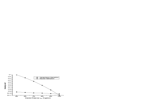
Figure 10: The Heisenberg and dipole-dipole spin interaction magnitudes as a function of interdot distance. The distance from the electrodes to the LHe surface $h=800\,\mathring{A}$ and the charges on the electrodes $Q_{A}=Q_{B}=1\,\mathrm{a.u.}$ The magnetic field $\vec{B}_{0}=0$.

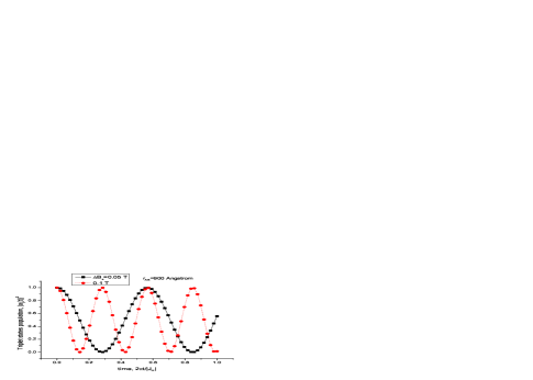
Figure 11: (color online) The triplet states population of electrons trapped in QDs on a LHe surface, as a function of time at different magnetic field differences $\Delta B_{z}=0.05$ and 0.1 T. Initially the system is in the triplet state $\left|S=1,M_{S}=0\right\rangle$. The distance between QDs is 900 Å. All other parameters are the same as in Fig. 10.

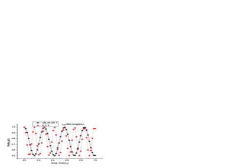
Figure 12: (color online) The purity $p(t)$ for the same parameters as in Fig. 11.

Figure 10 shows the magnitudes of the Heisenberg and dipole-dipole spin interaction, $|J_{H}|$ and $J_{\mathrm{dip}}$ from Eqs. (89) and (41) respectively, as a function of interdot distance. As estimated, the magnitude of the Heisenberg interaction is comparable to the weak dipole-dipole interaction at $r_{AB}\simeq 1000\,\mathrm{\mathring{A}}$. However, we remark that the strong dependence of $S\sim\exp(-\alpha r_{AB}^{2})$ (quadratic in the interdot distance) is due to the quadratic dependence on coordinates in the exponent of the corresponding oscillatory wavefunctions. Asymptotically, the confining potential Eq. (84) behaves as a 2D Coulomb potential, so that one should expect a milder coordinate dependence, $S\sim\exp(-\alpha r_{AB})$, at large distances (assuming $B_{0}=0$) and the rough estimate of Eq. (89) provides a lower bound for the Heisenberg interaction strength.

Lyon suggestedLyon06 using, instead of the exchange interaction, the magnetic dipole-dipole interaction between the spins in order to implement two-qubit gates, motivating this by the strong sensitivity of the exchange coupling to the parameters of the system and, hence, the corresponding difficulties with attempting to control this interaction. Our analysis confirms this, though, of course it is not easy to control the dipole-dipole interaction either: Eq. (41) shows that this interaction depends on only one controllable parameter, the interdot distance (the $g$-factor is a constant in vacuum).

Similarly to Figs. 1 and 2, Figs. 11 and 12 demonstrate non-unitary effects in the pure-spin model, due to magnetic field inhomogeneity in the electrons-on-LHe system. The interdot distance shown is $r_{AB}=900\,\mathrm{\mathring{A}}$. At this distance the Heisenberg interaction still prevails over the dipole interaction by at least an order of magnitude. Again, the pattern seen in the singlet-triplet states population redistribution is clearly oscillatory.

V Discussion and Conclusion

We have performed a comparative study of pure- and pseudo-spin dynamics for a system of two interacting electrons trapped in two QDs. We have shown that when there is negligible coupling between the spin and orbital degrees of freedom, which is the case of near $\vec{B}$-field homogeneity and negligible spin-orbit interaction, the system spin dynamics is unitary in both pure- and pseudo-spin models and is governed by the Zeeman interaction Hamiltonian of the total spin $\vec{S}$ ($S=1$) with the magnetic field $\vec{B}_{av}$. The singlet and triplet states are totally decoupled; the total spin is conserved. The spin system Hilbert space can be decomposed into two independent, singlet and triplet subspaces, the singlet spin states being magnetically inactive ($S=0$). Thus, the two-electron spin system restricted to the triplet subspace physically embodies a qutrit. The Heisenberg interaction operates differently in pure- and pseudo-spin models. If for simplicity we neglect double-occupancy states, the pseudo-spin state is totally defined by four complex amplitudes: $\left\{a_{s1}(0),a_{ti}(0),\,i=1,2,3\right\}$ in the basis $\{\Phi_{s1},\Phi_{ti}\}$; so that the Heisenberg interaction results in a phase unitary transformation: $\{a_{s1}(t)=\exp(-i\varepsilon_{s}t)a_{s1}(0),$ $a_{ti}(t)=\exp(-i\varepsilon_{t}t)a_{ti}(0)\}$. Since the spin-density matrix $\rho(t)$ is a bilinear combination of $a$’s: $\rho_{tij}(t)=a_{ti}(t)a_{tj}^{\ast}(t)$, $\rho_{s}(t)=1-\sum_{i}\rho_{tii}(t)$, the $\rho$-state will not by affected by the unitary transformation induced by the Heisenberg interaction.

We have also shown that unitary quantum gates realized in both spin models do not provide a universal set of gates under the condition $\Delta\vec{B}=0$. In order to obtain a universal set of gates, there should be both non-zero coupling between singlet and triplet states ($\Delta\vec{B}\neq 0$) and non-zero Heisenberg interaction ($J_{H}\neq 0$). Although at $\Delta\vec{B}\neq 0$ pure-spin dynamics becomes non-unitary, one can establish a relationship between unitary gates in pseudo-spin and the corresponding non-unitary gates in pure-spin dynamics so that a universal set of quantum gates constructed within the pseudo-spin model will generate a universal set of non-unitary gates in pure-spin dynamics.

To demonstrate the non-unitary effects, which are proportional to the square of the magnetic field inhomogeneity, in pure-spin dynamics, we have calculated how singlet and triplet states populations, as well as the purity and the Lamb energy shift, are affected by $\Delta\vec{B}\neq 0$ and spin-orbit interaction in $n$-doped GaAs semiconductors. These effects are found to be strongly dependent on the ratio of $\vec{B}$-field inhomogeneity and the Heisenberg interaction constant, $|\Delta B_{z}/J_{H}|$. For example, the singlet-triplet states population re-distribution is maximal at $t=\pi n/\omega$, where $\omega=\sqrt{J_{H}^{2}+\Delta B_{z}^{2}}$ and $n=1,3,\ldots$, and the singlet state population can achieve the value $\Delta B_{z}^{2}/\omega^{2}$. Thus, we can conclude that the Heisenberg interaction, characterized by the interaction constant $J_{H},$ plays an essential role in producing non-unitary effects in pure-spin dynamics. Spin-orbit interaction effects are found to be roughly four orders of magnitude smaller as compared to those caused by $\vec{B}$-field inhomogeneity.

As shown in Figs. 1-8, there are clear oscillations in the pure-spin dynamics and the non-unitary behavior of the spin-density matrix does not show the decaying pattern characteristic of a real decoherence process. This should be expected since the “bath” – the electron orbitals – in our spin model is not a real stochastic or infinite external bath, an interaction with which may result in irreversible decoherence. In essence, the spin dynamics is embedded in space and our bath is too small. The coordinate Hilbert space in the two-orbital ground state approximation adopted in the present paper is represented by 4 two-electron coordinate basis wavefunctions. In principle, the coordinate bath can be large in a system where couplings between excited and ground state orbitals are not negligible. This is an interesting question for future investigation: how will couplings to excited orbitals affect the non-unitary spin dynamics? The other interesting generalization of the present model is inclusion of real environment effects, i.e., the real stochastic bath representing the interaction of electron spins with the semiconductor medium. We will consider these and other generalizations in a future publications.

In the pseudo-spin model, where $\vec{B}$-field inhomogeneity results in first-order effects, we have estimated the contribution of the spin-orbit interaction to the effective pseudo-spin Hamiltonian, namely the Dzyaloshinskii-Moriya spin-orbit interaction term, and have suggested a two-step mechanism: coupling between the singly-occupied singlet state and triplet states occurs via intermediate, double-occupancy states (direct coupling between these states turns out to be zero due to orthogonality of the orbitals involved in the transition). Our calculations predict a smaller magnitude of the spin-orbit interaction as compared to the estimates of Ref. Kav01, , but are consistent with the results of Ref. GK03, .

In our second application we demonstrated, in Figs. 11 and 12, non-unitary effects due to $\Delta\vec{B}\neq 0$ in a system of electrons trapped above a liquid helium surface, namely the spin-based quantum computing proposal by Lyon Lyon06 . A more thorough investigation of spin dynamics in this system is left for a future publication.

In conclusion, we note that the two-electron spin-density matrix description advocated in this paper is expected to be useful when electrons trapped in QDs are not spatially resolved or resolvable. The spin-dynamics is then completely described by the spin-density matrix $\rho$. Although the $\rho$-dynamics becomes non-unitary in general (at $\Delta\vec{B}\neq 0$), it is controllable by modulating the interaction parameters, $J_{H}$, $\vec{B}_{av}$, $\Delta\vec{B}$. Since the non-unitarity comes from the magnetic field inhomogeneities, $\Delta\vec{B}$ and/or $\delta\vec{B}_{so}$, and since the $\rho$-dynamics is quadratically protected from these fields, this might prove to be important in practical quantum computing as minimizing coupling between spin and orbital degrees of freedom quadratically improves the fidelity of unitary gates in the $\rho$-state space.

References

• (1) D. Loss and D.P. DiVincenzo, Phys. Rev. A 57, 120 (1998).
• (2) B.E. Kane, Nature 393, 133 (1998).
• (3) R. Vrijen, E. Yablonovitch, K. Wang, H.W. Jiang, A. Balandin, V. Roychowdhury, T. Mor, and D. DiVincenzo, Phys. Rev. A 62, 012306 (2000).
• (4) X. Hu and S. Das Sarma, Phys. Rev. A 61, 062301 (2000).
• (5) J. Schliemann, D. Loss, and A.H. MacDonald, Phys. Rev. B 63, 085311 (2001).
• (6) X. Hu and S. Das Sarma, Phys. Rev. A 66, 012312 (2002).
• (7) B. Koiller, X. Hu, and S. Das Sarma, Phys. Rev. B 66, 115201 (2002).
• (8) T.A. Kaplan and C. Piermarocchi, Phys. Rev. B 70, 161311(R) (2004).
• (9) V.W. Scarola and S. Das Sarma, Phys. Rev. A 71, 032340 (2005).
• (10) L. He, G. Bester, and A. Zunger, eprint arXiv:cond-mat/0503492.
• (11) X. Hu, in Quantum Coherence: From Quarks to Solids, Vol. 689 of Lecture Notes in Physics (Springer, Berlin, 2006), p. 83.
• (12) J.M. Kikkawa, I.P. Smorchkowa, N. Samarth, and D.D. Awschalom, Science 277, 1284 (1997).
• (13) J.M. Kikkawa and D.D. Awschalom, Phys. Rev. Lett. 80, 4313 (1998).
• (14) J.A. Gupta, D.D. Awschalom, X. Peng, and A.P. Alivasatos, Phys. Rev. B 59, R10421 (1998).
• (15) D.D. Awschalom and N. Samarth, in Semiconductor Spintronics and Quantum Computation, edited by D.D. Awschalom, D. Loss, N. Samarth (Springer-Verlag, Berlin, 2002), pp. 147–193.
• (16) S.D. Kunikeev and D.A. Lidar, eprint arXiv:cond-mat/0708.0644.
• (17) K.V. Kavokin, Phys. Rev. B 64, 075305 (2001).
• (18) A. Auerbach, Interacting Electrons and Quantum Magnetism (Springer-Verlag, New-York, 1994).
• (19) J. Hubbard, Proc. Roy. Soc. London Ser. A 276, 238 (1963).
• (20) J. Hubbard, Proc. Roy. Soc. London Ser. A 277, 237 (1964).
• (21) J. Hubbard, Proc. Roy. Soc. London Ser. A 281, 401 (1964).
• (22) M. Takahashi, J. Phys. C 10, 1289 (1977).
• (23) A.H. MacDonald, S.M. Girvin, and D. Yoshioka, Phys. Rev. B 37, 9753 (1988).
• (24) I. Dzyaloshinskii, J. Phys. Chem. Solids 4, 241 (1958).
• (25) T. Moriya, Phys. Rev. 120, 91 (1960).
• (26) L. Jacak, P. Hawrylak, and A. Wójs, Quantum Dots (Springer-Verlag, Berlin, 1998).
• (27) A. Messiah, Quantum Mechanics, Vol. II (North-Holland Publishing Company, Amsterdam, 1962).
• (28) L.P. Gor’kov and P.L. Krotkov, Phys. Rev. B 67, 033203 (2003).
• (29) L.P. Gor’kov and L.P. Pitaevskii, Sov. Phys. Dokl. 8, 788 (1964).
• (30) C. Herring and M. Flicker, Phys. Rev. A 134, 362 (1964).
• (31) G. Dresselhaus, Phys. Rev. 100, 580 (1955).
• (32) Y.A. Bychkov and E.I. Rashba, J. Phys. C 17, 6039 (1984).
• (33) M. Abramowitz and I.A. Stegun (Eds.), Handbook of Mathematical Functions, 3rd Ed. (National Bureau of Standards, Applied Mathematical Series, USA, 1964).
• (34) M.I. Dyakonov and V.I Perel, Sov. Phys. Solid State 13, 3023 (1972).
• (35) J.C. Slater, Electronic Structure of Molecules (McGraw-Hill, New York, 1963).
• (36) R. Alicki and K. Lendi, Quantum Dynamical Semigroups and Applications, Lecture Notes in Physics, V. 286 (Springer-Verlag, Berlin, 1987).
• (37) D. Bacon, J. Kempe, D.A. Lidar and K.B. Whaley, Phys. Rev. Lett. 85, 1758 (2000).
• (38) J. Kempe, D. Bacon, D.A. Lidar, and K.B. Whaley, Phys. Rev. A 63, 042307 (2001).
• (39) D.A. Lidar and L.-A. Wu, Phys. Rev. Lett. 88, 017905 (2002).
• (40) J.F. Cornwell, Group Theory in Physics, V. II (Academic Press, London, 1990).
• (41) R.I. Dzhioev, K.V. Kavokin, V.L. Korenev, M.V. Lazarev, B.Ya. Meltser, M.N. Stepanova, B.P. Zakharchenya, D. Gammon, D.S. Katzer, eprint arXiv:cond-mat/0208083.
• (42) S.A. Lyon, Phys. Rev. A 74, 052338 (2006).
• (43) P.M. Platzman and M.I. Dykman, Science 284, 1967 (1999).
• (44) M.I. Dykman and P.M. Platzman, Fortschr. Phys. 48, 1095 (2000).
• (45) M.I. Dykman, P.M. Platzman, and Seddighrad, Phys. Rev. B 67, 155402 (2003).
• (46) M.I. Dykman, P.M. Platzman, and Seddighrad, Physica E 22, 767 (2004).