Length control of microtubules by depolymerizing motor proteins

Abstract

In many intracellular processes, the length distribution of microtubules is controlled by depolymerizing motor proteins. Experiments have shown that, following non-specific binding to the surface of a microtubule, depolymerizers are transported to the microtubule tip(s) by diffusion or directed walk and, then, depolymerize the microtubule from the tip(s) after accumulating there. We develop a quantitative model to study the depolymerizing action of such a generic motor protein, and its possible effects on the length distribution of microtubules. We show that, when the motor protein concentration in solution exceeds a critical value, a steady state is reached where the length distribution is, in general, non-monotonic with a single peak. However, for highly processive motors and large motor densities, this distribution effectively becomes an exponential decay. Our findings suggest that such motor proteins may be selectively used by the cell to ensure precise control of MT lengths. The model is also used to analyze experimental observations of motor-induced depolymerization.

I Introduction

In eukaryotic cells, microtubules (MT) are one type of cytoskeletal filaments, which perform several roles: they serve as tracks for intracellular molecular motor transport, provide structural rigidity to the cell and assemble to form a spindle during metaphase for the purpose of separation of duplicated chromosomes to the mother and daughter cells. MT are highly dynamic. In in vitro situations, it is observed that a growing MT can suddenly start shrinking; this “catastrophe” is triggered by the loss of the GTP cap by hydrolysis of GTP molecules attached to the tubulin subunits of MT. A shrinking MT occasionally get “rescued” and start polymerizing again. This unusual process of polymerization and depolymerization is referred to as ‘dynamic instability’  desai97 .

The situation inside the living cell is much more complex and the MT kinetics in vivo is regulated by many proteins. In particular, several motor proteins belonging to the kinesin family are now known to function as MT depolymerizers hunter00 ; moore05 ; kinoshita06 ; howard07 and are crucial in the formation and maintenance of the mitotic spindle wordeman05 . These include XKCM1/MCAK (mitotic centromere-associated kinesin) and Kif2A belonging to the kinesin-13 family and Kip3 proteins belonging to kinesin-8 family. MCAK is known to be active at kinetochores (the protein structure which facilitates MT attachment to chromosomes), whereas Kif2A is associated with centrosomes and Kip3p regulates microtubule-cortical interactions. Depletion/inhibition of XKCM1/MCAK has been shown to affect spindle length and the poleward motion of chromosomes during anaphase, while deletion of kinesin-8 proteins leads to defects in positioning of the spindlewordeman05 . However, the mechanism of depolymerization of MT by these motor proteins is only incompletely understood hunter03 .

Recent in vitro depolymerization experiments with surface-immobilized MT have demonstrated that the depolymerizing kinesins MCAK howard06 and Kip3p varga06 ; gupta06 use a ‘reduction of dimensionality’ mechanism to target the MT tips for depolymerization: after binding non-specifically to the MT surface, these proteins use diffusion (MCAK) or directed walk (Kip3p) to reach the tip(s), and their accumulation induces depolymerization of the MT from the tip. The depolymerization rate is, in general, length and motor-concentration dependent; in addition, MCAK and Kip3p are found to have vastly different residence times on the MT. These results indicate that depolymerizing kinesins could be used by the cell for precise length regulation of microtubules.

The central question of interest for us here is: what is the nature of the length-distribution of a set of microtubules in steady state, in a solution of free tubulin and depolymerizing motor proteins (henceforth referred to as depolymerizers for brevity)? In particular, it is important to understand how the depolymerizers contribute to the formation of a highly ordered structure such as the metaphase spindle, where most of the MT would need to be close to the spindle length. This aspect becomes significant, if we recall that the steady state length distribution of a set of microtubules undergoing dynamic instability under standard in vitro conditions has an exponentially decaying form, without any preferred length dogterom93 .

In this letter, we present a theoretical framework for understanding the depolymerizing activity of a generic motor protein as described above. After deriving expressions for the concentration profile of bound motors on a MT, we calculate the rate of absorption of motors at the MT tips. We then construct the rate equations for the length distribution(s) of MT, which are then solved perturbatively in the limits of low and high motor concentrations. We also show that the model can be used to analyze available experimental data on motor-induced depolymerization.

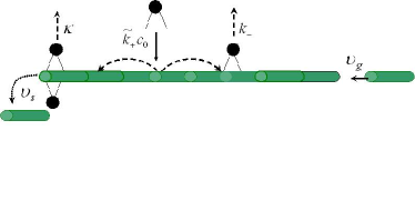
Figure 1: An illustration of our model, showing the important kinetic processes. Depolymerizer motor proteins attach to the surface of a MT and are transported along the MT by diffusion and/or directed walk. The motors are trapped at the MT tips, where they induce depolymerization of the MT. The MT grows at a motor-free tip by adding tubulin subunits. Bound motors may detach from the surface or the tips of the MT.

II Model description

Since we are interested in length-related properties, we consider here MT of finite length (unlike earlier theoretical approaches  klein05 ; howard06 to the problem, which concentrated on semi-infinite MT). In our model, a depolymerizer binds to a MT at a rate ${\tilde{k}}_{+}c_{0}$ per unit length ($c_{0}$ being the depolymerizer concentration in solution), and detaches at a rate $k_{-}$. A bound generic depolymerizer undergoes a biased random walk with drift speed $v_{0}$ and diffusion coefficient $D$. Once a depolymerizer reaches a tip of the MT, it depolymerizes the filament at a rate $v_{s}$ (measured in $\mu$m min^-1) while remaining attached to the tip. The depolymerizers accumulate at the tip, and detach from there at a rate ${\kappa}$, which characterizes its processivity(the tendency to stay attached to the MT tip while depolymerizing it). The tips, therefore, act as sinks for the depolymerizers which could accumulate there. The net rate of depolymerization, $v_{d}$, is a stochastic quantity, and depends on the number of accumulated motors. We further assume that a GTP cap is always present at a MT tip so that a depolymerizer-free tip will grow at a rate $v_{g}$ by adding tubulin sub-units (i.e., GTP hydrolysis is assumed to be sufficiently slow). An illustration of the model is provided in Fig. 1.

The MT-bound depolymerizer density profile will be denoted by $c(z,t)$ with $0\leq z\leq\ell$, $\ell$ being the length of the MT at time $t$. The kinetics of $c(z,t)$, in a frame of reference attached to the moving MT tip is given by the equation,

$$\frac{\partial c}{\partial t}=D\frac{\partial^{2}c}{\partial z^{2}}-v\frac{\partial c}{\partial z}-k_{-}c+{\tilde{k}}_{+}c_{0},$$ (1)

where $v=v_{0}-v_{m}$ and $v_{m}=v_{g}$ for a growing MT and $v_{m}=-v_{d}$ for a shrinking MT. Note that steric exclusion effects between motors have been neglected here for simplicity. In general, $v_{0}$ depends on $c$; however, at sufficiently small $c$, modification of the last term of eq.(1) to incorporate steric exclusion is equivalent to addition of just a constant to the detachment rate $k_{-}$klein05 .

So far as the surface transport on the MT is concerned, the MT tips act as “traps” for the depolymerases; however, a depolymerase can escape from the “trap” only by detachment from the MT during its MT-depolymerizing activity. Therefore, we treat the kinetics of the tip-absorbed motor population separately from the MT surface-bound (mobile) density of motors. The boundary conditions on $c(z,t)$, which are needed to solve eq. (1), should reflect the “trapping” of motors at the tips, and the simplest case is absorbing boundary conditions: $c(0,t)=c(\ell,t)=0$ for all $t$. Using time-independent boundary conditions requires that length fluctuations due to growth/shrinkage are sufficiently small, and the conditions for the same are derived now. We consider the $v_{0}=0$ case first. A single motor typically spends a residence time $\tau_{r}\sim 1/k_{-}$ on a sufficiently long MT ($\ell\gg\sqrt{D\tau_{r}}$), or otherwise gets absorbed at a tip within a shorter time interval $\sim\ell^{2}/D$. Clearly, only those motors that bind to the MT within a ‘depletion zone’ of length $\ell_{d}\sim\sqrt{D\tau_{r}}$ from a tip get absorbed at the tip, within a time interval $\sim\ell_{d}^{2}/D\sim\tau_{r}$, the rest will get detached before they can reach the tip. The length change over $\tau_{r}$ is $\delta\ell\sim v_{m}\tau_{r}$ with $v_{m}=v_{g}$ or $-v_{s}$, and the condition $|\delta\ell|\ll\ell$ is satisfied by $|v_{m}|\ll\sqrt{Dk_{-}}$. In the case of a motor which undergoes directed walk with velocity $v_{0}$, the corresponding condition turns out to be $|v_{m}|\ll v_{0}$.

Table 1: A list of experimental parameter values for MCAK howard06 and Kip3p  varga06 depolymerizers. The depolymerization rate is a function of length and motor concentration.

Quantity	MCAK	Kip3p
$D$	0.38 $\mu$m2s-1	-
$v_{0}$	-	3.6 $\mu$m min-1
$v_{d}$	$<4\mu$m min-1	$<2\mu$m min-1
${\tilde{k}}_{+}$	0.64nM${}^{-1}\mu$m-1s-1	assumed same
$k_{-}$	1.21 s-1	$\sim 0.004$s-1
$\kappa$	0.5s-1	0.03 s-1

Table 1 lists the various experimentally measured parameters for the two depolymerizers MCAK and Kip3p. For the purely diffusing MCAK, the above condition is satisfied for $|v_{m}|\ll 27\mu$m min^-1, and the analysis based on fixed boundary conditions should work well for growth rates of physiological interest. For walking Kip3p, the condition is marginally satisfied for low growth/shrinkage rates of $|v_{m}|\ll 1\mu$m min^-1. Nevertheless, we carry our analysis for the general case of a depolymerizer with directed motion as well as diffusion, assuming that the condition of small length fluctuations is satisfied. In particular, we will henceforth assume that $v\simeq v_{0}$ in eq. (1).

III Motor density profile and absorption rates

The steady-state density profile $c(z)$ of the motors, obtained from eq. (1), under the absorbing boundary conditions is

$$c(z)=K\bigg{[}1-\frac{1}{\sinh(\beta v\ell/2D)}\bigg{(}e^{-\frac{v(\ell-z)}{2D}}\sinh(\beta vz/2D)+$$

$$e^{\frac{vz}{2D}}\sinh(\beta v(\ell-z)/2D)\bigg{)}\bigg{]}$$ (2)

where $\beta=\sqrt{1+4Dk_{-}/v^{2}}$ and $K={\tilde{k}}_{+}c_{0}/k_{-}$. We emphasize that the function $c(z)$, being the density profile of only the motors not absorbed at the MT tips, vanish at $z=0$ and $z=\ell$. However, the total concentration of the depolymerizers at the MT tips is non-vanishing because of the accumulation of the absorbed depolymerizers there. We also note that eq. (2) is invariant under the combined transformations $v\to-v$ and $z\to\ell-z$.

It is interesting to look at the limiting behavior of the density profile in eq. (2) in the limits $v\to 0,D>0$ (pure diffusion) and $D\to 0,v>0$ (pure walk), since these special cases are of experimental interest. In the first case, the distribution has the following well-defined form, which is symmetric about $z=\ell/2$:

$$c_{d}(z)\equiv\lim_{v\to 0}c(z)=K\bigg{[}1-\frac{1}{\sinh(\ell/\lambda_{d})}\bigg{(}\sinh(z/\lambda_{d})+$$

$$\sinh((\ell-z)/\lambda_{d})\bigg{)}\bigg{]}~{}~{}~{};\lambda_{d}=\sqrt{D/k_{-}}$$ (3)

In the second case, after taking the limit $D\to 0$, we find that

$$c_{v}(z)\equiv\lim_{D\to 0}c(z)=K[1-\exp(-z/\lambda_{w})]~{}~{}~{}~{};\lambda_{w}=v/k_{-}$$ (4)

Note that eq. (4) is non-vanishing as $z\to\ell$, as expected for a pure directed walk towards the plus end. This does not contradict the imposed boundary conditions, because we still have $\lim_{D\to 0}\lim_{z\to l}c(z)=0$.

Since the kinetics at the minus end of a MT is typically much slower than that at the plus end, we concentrate only on the plus-end kinetics for the rest of this paper, though motor accumulation is allowed to occur at both ends. The rate of absorption of motors at the plus-end is given by $\nu(\ell)=-D(\partial c/\partial z)_{z=\ell}$, and has the general form:

$$\nu(\ell)=\frac{vK}{2\sinh(\beta v\ell/2D)}\bigg{[}\beta\bigg{(}\cosh(\beta v\ell/2d)-e^{v\ell/2D}\bigg{)}+$$

$$\sinh(\beta v\ell/2D)\bigg{]}.$$ (5)

$\nu(\ell)$ vanishes at $\ell=0$, and is a monotonically increasing function of $\ell$ for all values of $v$ and $D$. The saturation value for the general $v>0,D>0$ case is given by

$$\nu_{\max}=vK(1+\beta)/2.$$ (6)

For pure diffusion and pure walk, eq. (5) reduces, respectively, to the limiting forms,

$$\nu_{d}(\ell)={\tilde{k}}_{+}c_{0}\lambda_{d}\tanh(\ell/2\lambda_{d})~{}~{}~{}~{}~{};v\to 0$$ (7)

and

$$\nu_{v}(\ell)={\tilde{k}}_{+}c_{0}\lambda_{w}\left[1-\exp(-\ell/\lambda_{w})\right]=vc_{v}(l)~{}~{}~{}~{};D\to 0.$$ (8)

For short MT ($\ell\ll\lambda_{d}$ or $\lambda_{w}$ respectively), $\nu(\ell)\approx\frac{1}{2}{\tilde{k}}_{+}\ell$ in the first case and $\nu(\ell)\approx{\tilde{k}}_{+}\ell$ in the second; the difference of the factor of 2 arises from the fact that a diffusing depolymerizer can target either of the tips. In the opposite limit of long MT, both the rates approach their saturation values ${\tilde{k}}_{+}c_{0}\lambda_{d}$ and ${\tilde{k}}_{+}c_{0}\lambda_{w}$, respectively. (which may also be derived directly from eq. (6)).

IV Rate Equations

We will now study how a given depolymerizer would affect the length distribution of a set of MT, when a steady state is reached by a balance between depolymerizer binding/detachment and MT polymerization/depolymerization processes. For simplicity, we neglect the three-dimensional structure of the MT filament and imagine the MT as a linear polymer, made of sub-units of length $b$. We denote by $P_{n}(m,t)$ the fraction of polymers with $m$ sub-units and $n$ absorbed depolymerizers at the plus-end. Let $p_{g}=v_{g}/b$ be the probability per unit time for attachment of a subunit to a free tip and $p_{s}=v_{s}/b$ be the rate of removal of subunits per motor (we assume henceforth that the rate of sub-unit removal increases linearly with the number of motors). The rate equations for $P_{n}(m,t)$ are as follows: For $m=1$,

$$\frac{\partial P_{0}(1)}{\partial t}=-p_{g}P_{0}(1)+\kappa P_{1}(1),~{}~{}~{}~{}~{}~{}~{}~{}~{}~{}~{}~{}~{}~{}~{}~{}~{}~{}~{}~{}~{}~{}~{}~{}~{}$$

$$\frac{\partial P_{1}(1)}{\partial t}=p_{s}P_{1}(2)-\kappa P_{1}(1)+\nu(b)P_{0}(1),~{}~{}~{}~{}~{}~{}~{}$$ (9)

while for $m\geq 2$ and $n\geq 1$,

$$\frac{\partial P_{0}(m)}{\partial t}=-p_{g}[P_{0}(m)-P_{0}(m-1)]+$$

$$\kappa P_{1}(m)-\nu(mb)P_{0}(m)$$

$$\frac{\partial P_{n}(m)}{\partial t}=np_{s}[P_{n}(m+1)-P_{n}(m)]+$$

$$(n+1)\kappa P_{n+1}(m)+\nu(mb)P_{n-1}(m)-$$

$$(n\kappa+\nu(mb))P_{n}(m)~{}~{}~{}~{}~{}~{}~{}~{}$$ (10)

We now focus on the steady state of the model. Since a general analytic solution is difficult, we will adopt a perturbative approach, and look at the solutions in the limit of low and high depolymerizer concentrations. The transition between these regimes is controlled by the dimensionless ratio $\eta=\nu_{\max}/\kappa$ which may be used as the small parameter in the low density perturbation expansion. This is seen through the following argument.

Let us define a distribution of the number of accumulated motors: $\chi_{n}\equiv\sum_{m=1}^{\infty}P_{n}(m)$. It is convenient to use the numbers $\alpha_{n}<1$, defined through the relation $\sum_{m=1}^{\infty}\nu(mb)P_{n}(m)\equiv\nu_{\max}\alpha_{n}\chi_{n}$. From eq.( 9) and eq.( 10), it can be shown that, in steady state, $\chi_{n}$ follows a Poisson-like distribution of the form $\chi_{n}=\chi_{0}(\eta^{n}/n!)\prod_{i=0}^{n-1}\alpha_{i}$ for $n\geq 1$, where $\chi_{0}$ is determined through normalization: $\sum_{n=0}^{\infty}\chi_{n}=1$.

Low motor concentration: For $\eta\ll 1$, we can neglect $P_{n}$ with $n\geq 2$ in eq. (10), in comparison with $P_{0}$ and $P_{1}$. By keeping terms upto $O(\eta)$, in the continuum limit ($m\gg 1,\ell\approx mb$), we arrive at a single combined equation for $P_{0}$ and $P_{1}$ in steady state:

$$v_{g}\frac{\partial P_{0}}{\partial\ell}=-\nu(\ell)P_{0}(\ell)+\kappa P_{1}(\ell)=v_{s}\frac{\partial P_{1}}{\partial\ell}$$ (11)

which has the general solution (for $\ell\gg b$)

$$P_{0}(\ell)=C\exp\bigg{(}\frac{\kappa}{v_{s}}\ell-\frac{1}{v_{g}}\int_{0}^{\ell}\nu(\ell^{\prime})d\ell^{\prime}\bigg{)}=\frac{v_{s}}{v_{g}}P_{1}(\ell)$$ (12)

where $C$ is a constant of normalization. In the absence of a boundary, this solution is normalizable only when $\eta>\eta_{c}$, where $\eta_{c}=v_{g}/v_{s}$ implicitly gives a critical motor concentration, below which a well-defined steady state distribution does not exist. The above result for $\eta_{c}$ is, however, strictly true only when $v_{g}/v_{s}\ll 1$ since the present analysis assumes $\eta\ll 1$. In the more general case, a steady state should still exist at sufficiently large $\eta$, but the critical concentration would be given by a relation of the form $\eta_{c}=f(v_{g}/v_{s})$, with $f(x)\simeq x$ as $x\to 0$.

High motor concentration: To analyze the case $\eta\gg 1$, it is convenient to re-express eq. (9) and eq. (10) (in the continuum limit) as

$$\frac{v_{g}}{\nu_{\max}}\frac{\partial P_{0}}{\partial\ell}=\eta^{-1}P_{1}(\ell)-f(\ell)P_{0}(\ell)$$

$$-\frac{nv_{s}}{\nu_{\max}}\frac{\partial P_{n}}{\partial\ell}=(n+1)\eta^{-1}P_{n+1}(\ell)+f(l)P_{n-1}(\ell)-$$

$$(n\eta^{-1}+f(\ell))P_{n}(\ell),$$ (13)

where the function $f(\ell)\equiv\nu(\ell)/\nu_{\max}\leq 1$. We now expand all $P_{n}(l)$ in a perturbation series in $\eta^{-1}$: $P_{n}(\ell)=\sum_{m=0}^{\infty}\eta^{-m}P_{n}^{(m)}(\ell)$ for $n\geq 0$, and then substitute into eq. (13). The zeroth order distributions are then found to satisfy the iterative equation,

$$-\frac{nv_{s}}{\nu_{\max}}\frac{\partial P_{n}^{(0)}}{\partial\ell}=f(\ell)[P_{n-1}^{(0)}(\ell)-P_{n}^{(0)}(\ell)]$$ (14)

and $P_{0}^{(0)}(\ell)=P_{0}^{(0)}(0)\exp(-v_{g}^{-1}\int_{0}^{\ell}d{\ell}^{\prime}\nu(\ell^{\prime}))$ from eq. (13). The solution of eq. (14) is found after a few elementary calculations:

$$P_{n}^{(0)}(\ell)=P_{n}^{(0)}(0)e^{-\frac{1}{v_{g}}\int_{0}^{\ell}d\ell^{\prime}\nu(\ell^{\prime})}.$$ (15)

where

$$P_{n}^{(0)}(0)=P_{0}^{(0)}(0)\prod_{m=1}^{n}\frac{v_{g}}{v_{g}+mv_{s}}.$$ (16)

The unknown constant $P_{0}^{(0)}$ is determined by normalization. Eq. (15) is a monotonically decreasing function of $\ell$, however, non-monotonic terms appear in the first order and above.

\psfrag{'fort.12'}{$\zeta=1.2$}\psfrag{'fort.16'}{$\zeta=1.6$}\psfrag{'fort.20'}{$\zeta=2.0$}\psfrag{P(x)}{$P_{0}(x)$}\psfrag{<x>}{$\langle x\rangle$}\psfrag{x}{$x$}\psfrag{c}{$\zeta$}\includegraphics[width=151.76633pt]{FIG2.ps}

\psfrag{'fort.12'}{$\zeta=1.2$}\psfrag{'fort.16'}{$\zeta=1.6$}\psfrag{'fort.20'}{$\zeta=2.0$}\psfrag{P(x)}{$P_{0}(x)$}\psfrag{<x>}{$\langle x\rangle$}\psfrag{x}{$x$}\psfrag{c}{$\zeta$}\includegraphics[width=86.72267pt]{FIG2inset.ps}

Figure 2: The distribution in eq. (17) (normalized such that $\int P_{0}(\ell)d\ell=1$) is plotted against the dimensionless ‘length’ $x=\ell/2\lambda_{d}$(eq. (3)) for three different values of $\zeta=\eta/\eta_{c}$. The other parameters were fixed at the MCAK values (table 1). We assumed $v_{s}\simeq v_{d}$ and $v_{g}\simeq 1\mu$m min^-1. From table 1, $\lambda_{d}\simeq 0.56\mu$m for MCAK. Inset: the mean length as a function of $\zeta$ (computed numerically, $\delta x=10^{-5}$ everywhere). Using the parameters in table 1, the critical MCAK concentration corresponding to $\eta_{c}$ is $~{}1.39v_{g}/v_{s}$ nM.

\psfrag{'fort.12'}{$\zeta=1.2$}\psfrag{'fort.16'}{$\zeta=1.6$}\psfrag{'fort.20'}{$\zeta=2.0$}\psfrag{P(x)}{$P_{0}(x)$}\psfrag{<x>}{$\langle x\rangle$}\psfrag{x}{$x$}\psfrag{c}{$\zeta$}\includegraphics[width=151.76633pt]{FIG3.ps}

\psfrag{'fort.12'}{$\zeta=1.2$}\psfrag{'fort.16'}{$\zeta=1.6$}\psfrag{'fort.20'}{$\zeta=2.0$}\psfrag{P(x)}{$P_{0}(x)$}\psfrag{<x>}{$\langle x\rangle$}\psfrag{x}{$x$}\psfrag{c}{$\zeta$}\includegraphics[width=86.72267pt]{FIG3inset.ps}

Figure 3: Similar to the previous figure, using the distribution in eq.(18) and Kip3p parameter values (table 1). Here, $x=\ell/\lambda_{w}$ (eq.(4))with $\lambda_{w}\simeq 15\mu$m for Kip3p. The critical Kip3p concentration corresponding to $\eta_{c}$ is $\sim 0.003v_{g}/v_{s}$ nM.

V Application to specific cases

Our results so far have been general, within the limits of validity of the assumptions stated in the second section. We will now examine their implications for the specific depolymerizer motor proteins studied in experiments.

The solution obtained in eq. (12) in the limit of low concentrations is a non-monotonic function of the length, increasing exponentially as $\sim e^{(\kappa/v_{s})\ell}$ for small $\ell$, and decreasing exponentially at large $\ell$, with a peak at an intermediate value. The location of this peak depends on the ratio $\kappa/v_{s}$, and for fixed $v_{s}$, the peak is more pronounced for large $\kappa$ (low processivity) and vice-versa. The depolymerizers MCAK and Kip3p have very different processivities (table 1), and it is therefore interesting to look at these specific cases in more detail. Eq. (12) reduces to the following forms in the pure diffusion ($v\to 0,D>0$) and pure walk ($v>0,D\to 0$) limits respectively:

$$P_{0}(\ell)\propto e^{\kappa\ell/v_{s}}\left[\cosh(\ell/2\lambda_{d})\right]^{-\frac{2K\lambda_{d}^{2}}{v_{g}}}~{}(v_{0}=0)$$ (17)

$$P_{0}(\ell)\propto\exp\left[\bigg{(}\frac{\kappa}{v_{s}}-\frac{K\lambda_{w}}{v_{g}}\bigg{)}\ell-\frac{K\lambda_{w}^{2}}{v_{g}}e^{-\ell/\lambda_{w}}\right](D=0)$$ (18)

\psfrag{fluct}{$\frac{\Delta x}{\langle x\rangle}$}\psfrag{c}{$\zeta$}\includegraphics[width=130.08731pt]{FIG4.ps}

Figure 4: The ratio of the standard deviation to the mean length of the distributions in fig.2 and fig.3 as a function of $\zeta=\eta/\eta_{c}$.

Fig. 2 and fig. 3 show the normalized forms of the distributions in eq. (17) and eq. (18) respectively, plotted against the dimensionless length variables $x=\ell/\lambda_{d}$ and $x=\ell/\lambda_{w}$, for three values of $\zeta=\eta/\eta_{c}>1$ (the empirical values of $\kappa,D,v_{0}$ and $v_{s}$ are taken from Table 1). Although, as we explained in the beginning, our theory is more applicable to MCAK than Kip3p, the difference between the two cases is nevertheless striking: the MCAK distribution shows a peak, while the Kip3p distribution is essentially a monotonically decreasing function (the peak is too close to the origin to be visible in the plot). The contrasting behavior is primarily due to their very different processivities.

In order to characterize the MCAK and Kip3p-induced distributions better, we also looked at how the lengths are spread about the mean value in each of these cases. In fig. 4, we plot the relative MT length fluctuation $\Delta x/\langle x\rangle$ for MCAK and Kip3p, as a function of the dimensionless ratio $\zeta=\eta/\eta_{c}$, where $\Delta x=\sqrt{\langle x^{2}\rangle-\langle x\rangle^{2}}$ is the standard deviation. The relative fluctuation for MCAK is typically smaller than 1, and, interestingly, also shows a minimum of $\sim 0.3$ at $\zeta\simeq 1.37$. For Kip3p, on the other hand, the relative fluctuation increases rapidly with $\zeta$ and saturates at unity, which is characteristic of a purely exponential distribution. MCAK appears to produce a tighter control of length than Kip3p because of its lower processivity.

VI Length-dependent depolymerization

\psfrag{'fort.12'}{$\zeta=1.2$}\psfrag{'fort.16'}{$\zeta=1.6$}\psfrag{'fort.20'}{$\zeta=2.0$}\psfrag{n}{$\langle n\rangle_{\ell}$}\psfrag{l}{$\ell$($\mu$m)}\psfrag{c}{$c_{0}$(nM)}\psfrag{'conc1'}{1nM}\psfrag{'fort.15'}{4nM}\psfrag{'fort.16'}{$\ell$=5$\mu$m}\includegraphics[width=151.76633pt]{FIG5.ps}

\psfrag{'fort.12'}{$\zeta=1.2$}\psfrag{'fort.16'}{$\zeta=1.6$}\psfrag{'fort.20'}{$\zeta=2.0$}\psfrag{n}{$\langle n\rangle_{\ell}$}\psfrag{l}{$\ell$($\mu$m)}\psfrag{c}{$c_{0}$(nM)}\psfrag{'conc1'}{1nM}\psfrag{'fort.15'}{4nM}\psfrag{'fort.16'}{$\ell$=5$\mu$m}\includegraphics[width=86.72267pt]{FIG5inset.ps}

Figure 5: The figure shows the mean number of tip-absorbed motors (computed numerically using eq. 19), plotted as a function of the MT length for MCAK, for two values of the bulk motor concentration $c_{0}$. The inset shows the saturation value (computed at $\ell=5\mu$m) plotted against $c_{0}$.

We will now focus on the analysis of the existing experimental results on motor-induced depolymerization within our model. The rate of depolymerization of a microtubule depends on the number $n$ of motor proteins accumulated at the tip. Experiments with fixed microtubule length measure the mean depolymerization rate $\langle v_{d}\rangle=v_{s}\langle n\rangle_{\ell}$, where $\langle n\rangle_{\ell}$ gives the mean number of motors attached to a microtubule of length $\ell$. To calculate this average, we define the distribution $Q_{\ell}(n)$ for the number of motors attached to the tip of a MT of length $\ell$. We assume that a motor protein initially bound to one protofilament will continue to travel along it until it reaches a tip, without hopping between filaments. In this case, absorption at a certain protofilament tip is possible only if that particular tip is free, the probability of which is given by $(1-n/n^{*})$, where $n$ is the total number of motors attached at the MT tip and $n^{*}$ is the maximum number of motors that can be absorbed at a given time. Since a MT usually has 13 protofilaments, we assume $n^{*}=13$ for concreteness.

The rate equations for $Q_{\ell}(n)$ are as follows. For motor-free tips, we have

$$\frac{\partial Q_{\ell}(0)}{\partial t}=\kappa Q_{\ell}(1)-\nu(\ell)Q_{\ell}(0)$$

$$\frac{\partial Q_{\ell}(n)}{\partial t}=(n+1)\kappa Q_{\ell}(n+1)+$$

$$\nu(\ell)\bigg{(}1-\frac{n}{n^{*}}\bigg{)}\bigg{[}Q_{\ell}(n-1)-Q_{\ell}(n)\bigg{]}+$$

$$Q_{\ell}(n-1)\frac{\nu(l)}{n^{*}}-n\kappa Q_{\ell}(n)~{}~{}~{}~{};1\leq n<n^{*}$$

$$\frac{\partial Q_{\ell}(n^{*})}{\partial t}=-n^{*}\kappa Q_{\ell}(n^{*})+\frac{\nu(\ell)}{n^{*}}Q_{\ell}(n^{*}-1)$$ (19)

The steady state solution of eq. (19) is given by

$$Q_{\ell}(n)=Q_{\ell}(0)\frac{1}{n!}\bigg{(}\frac{\nu(\ell)}{\kappa}\bigg{)}^{n}\prod_{j=1}^{n-1}(1-\frac{j}{n^{*}})~{}~{}~{}~{}1\leq n\leq n^{*}$$ (20)

where $Q_{\ell}(0)$ is fixed by normalization: $\sum_{n=1}^{n^{*}}Q_{\ell}(n)=1$. The mean number of tip-accumulated motors is then given by $\langle n\rangle_{\ell}=\sum_{n=1}^{n^{*}}nQ_{\ell}(n)$.

\psfrag{n}{$\langle n\rangle_{\ell}$}\psfrag{l}{$\ell$($\mu$m)}\includegraphics[width=151.76633pt]{FIG6.ps}

Figure 6: The average number of tip-absorbed motors in the presence of Kip3p, for three different values of $c_{0}$. Note the difference in length scales between this and the previous figure.

In fig. 5, we have plotted numerically computed $\langle n\rangle_{\ell}$ as a function of $\ell$ in the case of MCAK for two different motor concentrations $c_{0}$. It is found that appreciable length-dependence of $\langle n\rangle_{\ell}$, and hence the mean depolymerization velocity $\langle v_{d}\rangle$, is found only for $\ell<2\mu$m. This is in agreement with experiments, where no length-dependence of depolymerization was observed in the case of MCAK, for MT longer than 2$\mu$m. The saturation value of the depolymerization rate (plotted in the inset, for $\ell=5\mu$m) depends strongly on the motor concentration, and this curve also agrees well with experimental results howard06 and previous theoretical predictions klein05 .

We now turn to the case of Kip3p, in which case a strong length-dependence of depolymerization was observed in experiments varga06 . Fig. 6 shows the theoretical plot of $\langle n\rangle_{\ell}$ against $\ell$ for three motor concentrations. The length-dependence here is much stronger than MCAK, and for low concentrations, saturation is not reached even for $\ell=20\mu$m. These observations qualitatively agree with the corresponding experimental results. However, a close quantitative agreement (in particular, experiments show a sharp rise in depolymerization rate between $c_{0}$=3.3nM and $c_{0}$=5.8nM) is missing in this case.

VII Conclusions

To conclude, in this letter, we have formulated a general theory for the action of MT-depolymerizing motor proteins. Specifically, we considered the limit where the motor density profile becomes stationary much before the MT length distribution reaches its steady-state. We showed that the rate of accumulation of the motors at the MT tips, and consequently their depolymerizing activity itself, is strongly length-dependent. This has a rather pronounced effect on the length distribution of the MT, which displays a peak before decaying exponentially at large $\ell$. Interestingly, the processivity of the depolymerizer plays an important role in determining the nature of the length distribution: a depolymerizer with low processivity produces a more pronounced peak in the length distribution, and is likely to be more useful for precise length regulation.

Our theory is relevant to future experimental studies on the role of depolymerizing motor proteins in length regulation of MT, especially in the context of formation of the metaphase spindle. Indeed, very recent experiments using fluroscent speckle microscopy have shown that the length distribution of individual MT in a meiotic spindle is strongly non-monotonic yang07 . It would be interesting if the predictions made in this paper could be put to test in future in vitro experiments with depolymerizing motor proteins, where the MT lengths are carefully monitored.

- (1) Desai A. and Mitchison. T.J., Annu. Rev. Cell. Dev. Biol.13, 83 (1997).
- (2) Hunter A.W. and Wordeman L., J. Cell Sci.113, 4379 (2000).
- (3) Moore A.T. et al, J. Cell Biol. 169, 391 (2005).
- (4) Kinoshita K. et al, J. Mus. Res. Cell. Mot.27, 107 (2006).
- (5) Howard J. and Hyman A.A., Curr. Opin. Cell Biol.19, 31 (2007).
- (6) Wordeman L., Curr. Opin. Cell Biol.,17, 82 (2005).
- (7) Hunter A.W. et al, Mol. Cell11, 445 (2003).
- (8) Helenius J. et al, Nature 441, 115 (2006).
- (9) Varga V. et al, Nat. Cell Biol 8, 957 (2006).
- (10) Gupta M. L. et al, Nat. Cell Biol.8, 913 (2006).
- (11) Dogterom M. and Leibler S., Phys. Rev. Lett.70, 1347 (1993).
- (12) Klein G. A. et al, Phys. Rev. Lett.94, 108012 (2005).
- (13) Yang G. et al, Nat. Cell Biol.9(11), 1233(2007).