Numerical simulations of the type III migration:
I. Disc model and convergence tests

Abstract

We investigate the fast (type III) migration regime of high-mass protoplanets orbiting in protoplanetary disks. This type of migration is dominated by corotational torques. We study the the details of flow structure in the planet’s vicinity, the dependence of migration rate on the adopted disc model, and the numerical convergence of models (independence of certain numerical parameters such as gravitational softening).

We use two-dimensional hydrodynamical simulations with adaptive mesh refinement, based on the FLASH code with improved time-stepping scheme. We perform global disk simulations with sufficient resolution close to the planet, which is allowed to freely move throughout the grid. We employ a new type of equation of state in which the gas temperature depends on both the distance to the star and planet, and a simplified correction for self-gravity of the circumplanetary gas.

We find that the migration rate in the type III migration regime depends strongly on the gas dynamics inside the Hill sphere (Roche lobe of the planet) which, in turn, is sensitive to the aspect ratio of the circumplanetary disc. Furthermore, corrections due to the gas self-gravity are necessary to reduce numerical artifacts that act against rapid planet migration. Reliable numerical studies of Type III migration thus require consideration of both the thermal and the self-gravity corrections, as well as a sufficient spatial resolution and the calculation of disk-planet attraction both inside and outside the Hill sphere. With this proviso, we find Type III migration to be a robust mode of migration, astrophysically promising because of a speed much faster than in the previously studied modes of migration.

1 Introduction

In the standard model of planetary system formation giant planets form through core accretion outside the ice condensation boundary ($4-5$ AU), where the availability of water ice allows planetary cores to rapidly reach the critical mass of $\sim$10 Earth masses, beyond which substantial gas accretion can occur (Pollack et al., 1996). This theory provides a good fit to the structure of the Solar System, but does not explain the presence of so-called ‘hot Jupiters’ (objects with minimum masses similar to or larger than Jupiter’s mass, $M_{\jupiter}$, and semi-major axes $a<0.1$ AU) discovered in extrasolar planetary systems (Mayor & Queloz 1995, Marcy et al. 2000, Vogt et al. 2002). Since the in situ formation of these objects is difficult both in the core accretion scenario and through direct gravitational instability (Boss, 2001), the inward migration of bodies and eccentricity pumping due to planet-planet and planet-remnant disc interaction become important parts of the new theory of planet formation.

The standard theory of planet migration (Goldreich & Tremaine 1979, 1980; Lin & Papaloizou 1993; Lin et al. 2000) considers the Lindblad resonances and neglects the corotational resonances, assuming a smooth initial density profile in the disc and a small density gradient at the corotation radius. Tidal torques due to the Lindblad resonances are believed to cause inward migration of a planet (type I or type II, for low and high mass planets respectively) from the region where it formed to the inner regions where many exoplanets are observed. The type II migration times for giant planets are essentially viscous time-scales of disks, thus relatively long (Ward, 1997).

However, it was recently found that the corotational resonance can modify the type I migration mode (Masset et al. 2006, Paardekooper & Mellema 2006) or lead to a new and very fast migration mode (type III, or run-away migration) that depends strongly on the gas flow in the planet’s vicinity and does not have a predetermined direction (Masset & Papaloizou 2003; Artymowicz 2004; Papaloizou 2005; Artymowicz 2006). This type of migration was studied numerically by Masset & Papaloizou (2003) who performed two-dimensional simulations of a freely migrating planet and a steady state migration with fixed migration rate $\dot{a}$ for a range of the migration rates. Global, high resolution two- and three-dimensional simulations of freely migrating planets were performed by D’Angelo et al. (2005). Papaloizou (2005) considered local shearing box simulations.

These numerical simulations showed that the planet’s orbital evolution depends strongly on the choice of the simulation parameters, e.g. grid resolution (D’Angelo et al., 2005), softening of the planet gravitation potential, etc. The reason for this dependence can be the simplifications commonly used in the disc model. The most important simplifications are the use of two-dimensional simulations, ignoring self-gravity and the local-isothermal approximation, that imposes a static temperature distribution in the planet’s vicinity.

This is the first in a series of papers devoted to type III migration of high-mass protoplanets interacting with the protoplanetary disc. In this paper we study the dependence of the planet migration on the applied disc model and we defer the description of the physics of type III migration itself to Peplinski et al. (2007a) and Peplinski et al. (2007b) (henceforth Paper II and Paper III). We concentrate on two aspects: a modification of the local-isothermal approximation, that allows an increase the temperature inside the Roche lobe, and a correction of the gas acceleration (due to the gas self-gravity) that forces the circumplanetary disc to move together with the planet.

In order to analyse this we study the gas flow in the planet’s vicinity by performing numerical hydrodynamical simulations in two dimensions of a gaseous disc interacting with the star and one planet. The planet is allowed to migrate due to disc-planet interaction and we can study its orbital evolution in the non-steady state. Since type III migration is so sensitive to the gas flow near the planet, we include a careful analysis of the effects of various numerical parameters which influence these flow patterns.

The layout of the paper is as follows. In Sections 2 and 3 we give the basic equations, describe the disc model and the numerical method. Sections 4 and 5 contain the convergence tests and a discussion of the effects of various modifications of disc model and numerical parameters for inward and outward migration. Finally in Section 6 we discuss their implications for numerical simulations of type III migration.

2 Description of the physical model

2.1 Disc model

We adopt in our simulations a two-dimensional, infinitesimally thin disc model and use vertically averaged quantities, such as the surface mass density

$$\Sigma=\int\limits_{-\infty}^{\infty}\rho\,\mathrm{d}z,$$ (1)

where $\rho$ is the mass density. We work in the inertial reference frame, in a Cartesian coordinate system $(x,y,z)$, also see Sect. 3.2. The plane of the disc and the star-planet system coincides with the $z=0$ plane. The centre of mass of the star- planet system is initially set at the origin of the coordinate system. Since the star and the planet are allowed to migrate freely due to the gravitational interaction with the disc, and the total angular momentum of the whole system is not fully conserved due to the open boundary conditions (see Section 2.3.2), the centre of mass can move slowly away from the origin of the coordinate system. The positions and masses of the star and the planet we denote by $\mn@boldsymbol{r}_{\mathrm{S}}$, $M_{\mathrm{S}}$, $\mn@boldsymbol{r}_{\mathrm{P}}$ and $M_{\mathrm{P}}$ respectively.

The gas in the disc is taken to be inviscid and non-self-gravitating. The evolution of the disc is given by the two-dimensional $(x,y)$ continuity equation for $\Sigma$ and the Euler equations for the velocity components $\mn@boldsymbol{v}\equiv(v_{x},v_{y})$. These equations can be written in conservative form as

$${\partial\Sigma\over\partial t}+\nabla(\Sigma\mn@boldsymbol{v}) = 0,$$ (2)

$${\partial\Sigma\mn@boldsymbol{v}\over\partial t}+\nabla(\Sigma\mn@boldsymbol{v}\mn@boldsymbol{v})+\nabla P = -\Sigma\nabla\Phi,$$ (3)

where $P$ is two-dimensional (vertically integrated) pressure, and $\Phi$ is the gravitational potential generated by protostar (subscript S) and planet (subscript P)

$$\Phi=\Phi_{\mathrm{S}}+\Phi_{\mathrm{P}}=-{GM_{\mathrm{S}}\over|\mn@boldsymbol{r}-\mn@boldsymbol{r}_{\mathrm{S}}|}-{GM_{\mathrm{P}}\over|\mn@boldsymbol{r}-\mn@boldsymbol{r}_{\mathrm{P}}|}.$$ (4)

We do not consider the energy equation, since we use a local isothermal approximation (see Sect. 2.1.1).

The gravitational potential close to the star and the planet is softened in the following way:

$$\widetilde{\Phi}=\left\{\begin{array}[]{ccc}{-GM\over r}&\hbox{; for }\xi>1\\ \\ {-GM\over r_{\mathrm{soft}}}(1.875\xi^{6}-7\xi^{5}+7.875\xi^{4}+\\ -4.375\xi^{2}+2.625)&\hbox{; for }\xi\leq 1\end{array}\right.$$ (5)

where $\xi=r/r_{\mathrm{soft}}$ and $r_{\mathrm{soft}}$ is the so-called smoothing length (or gravitational softening). The reason for using this formula instead of the standard one (where $r$ and $r_{\mathrm{soft}}$ are added geometrically) is to remove the dependence of the Keplerian speed on the gravity smoothing length for $r>r_{\mathrm{soft}}$ in the disc surrounding the body. This is especially important for simulations using a Cartesian grid since the stellar gravity has to be softened too. Moreover it allows for a bigger smoothing length around the planet without influencing the outer part of the Roche lobe. This is necessary because the planet is moving across the grid and its position with respect to cell centres varies. As Nelson & Benz (2003a) pointed out, in this case, in order to avoid unphysical effects on the planet’s trajectory caused by close encounters with cell centres, the smoothing length needs to be larger than half the dimension of the cell. In our simulations $r_{\mathrm{soft}}$ is at least a few times the cell size.

Unlike the standard formula for softening of the gravity, our formula corresponds to a spherical body with a finite radius given by $r_{\mathrm{soft}}$. The internal structure of this body can be found using the Poisson equation and is given by the formula

$$\varrho_{\mathrm{soft}}=\left\{\begin{array}[]{ccc}{0}&\hbox{; for }\xi>1\\ \\ {M\over{4\pi r_{\mathrm{soft}}^{3}}}(-78.75\xi^{4}+210\xi^{3}+\\ -157.5\xi^{2}+26.25)&\hbox{; for }\xi\leq 1\end{array}\right.$$ (6)

Since $r=r_{\mathrm{soft}}$ is the “surface” of the body generating the gravitational potential, we will include the mass of the gas within the gravitational softening $M_{\mathrm{soft}}$ to the effective planet mass. For more discussion see Sections 2.1.2 , 5.1.2 and 5.2.2.

Previous studies of migrating Jupiter-mass planets showed that an important issue is the treatment of the torques arising from within the Hill sphere (Nelson & Benz 2003b; D’Angelo et al. 2005). It is often assumed that these torques are strong, but nearly cancel, and thus can be neglected. In addition it has been argued that accelerating a planet through its own (bound) envelope would be unphysical. In general, the exclusion of the torques arising from within the Hill sphere is inconsistent, but can be justified if the density distribution in the Hill sphere is (almost) static and if the circumplanetary disc can be considered as a separate system. As we show below, these assumptions are not necessarily satisfied in the highly dynamic case of type III migration. The torques from the planet’s vicinity need be taken into account. Obviously, these torques depend strongly on the density distribution near the planet, which in a numerical simulation will depend on a combination of the resolution and the parameters determining this density distribution. The gravitational softening $r_{\mathrm{soft}}$ is one of these parameters. In Sect. 5.1.1 we study the effects of gravitational softening.

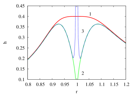
Figure 1: The real disc aspect ratio calculated with respect to the planet for two formulae for isothermal sound speed $c_{\mathrm{s}}$. Curve 1: EOS2 (Eq. 11); curve 2: EOS1 (Eq. 10). Curve 3 shows the real aspect ratio for EOS2 after taking into account the gravitational softening (the result for EOS1 is not affected by this).

2.1.1 Equation of state

Since a self-consistent calculation of the temperature is prohibitively expensive, we adopt the usual local isothermal approximation: the disc is treated as a system having a fixed temperature distribution. In this case the equation of state has the form

$$P=c_{\mathrm{s}}^{2}\Sigma,$$ (7)

$c_{\mathrm{s}}$ being the local isothermal sound speed. The thermal state of the fluid is given by $c_{\mathrm{s}}$, which is usually assumed to be a power law of the distance to the star $r_{\mathrm{s}}=|\mn@boldsymbol{r}-\mn@boldsymbol{r}_{\mathrm{S}}|$. Assuming that the material inside a circumstellar disc is in hydrostatic equilibrium and neglecting the planet gravitational field, we can get the simple, widely used formula

$$c_{\mathrm{s}}=H\Omega_{\mathrm{s}},$$ (8)

where $H$ is the disc scale height and $\Omega_{\mathrm{s}}$ is the Keplerian angular velocity in the circumstellar disc

$$\Omega_{\mathrm{s}}=\sqrt{GM_{\mathrm{S}}\over r_{\mathrm{s}}^{3}}.$$ (9)

This formula, for the constant disc opening angle, gives

$$c_{\mathrm{s}}=h_{\mathrm{s}}r_{\mathrm{s}}\Omega_{\mathrm{s}},$$ (10)

where $h_{\mathrm{s}}=H/r_{\mathrm{s}}$ is the disc aspect ratio with respect to the star. In this case the Mach number of the flow in the disc is a constant given by $1/h_{\mathrm{s}}$. We will designate this choice as EOS1 (equation of state 1).

For EOS1 the gas temperature is not modified by the presence of the planet. Because of the gravitational field of the embedded planet, the disc aspect ratio calculated with respect to the planet $h_{\mathrm{p}}=H/|\mn@boldsymbol{r}-\mn@boldsymbol{r}_{\mathrm{P}}|$ can achieve very small values (see Fig. 1), allowing the planet to collect large amounts of material. Physically, we should expect a temperature increase in the vicinity of a Jupiter-mass planet. Two-dimensional simulations (D’Angelo et al., 2003) showed that an accreting Jupiter on a constant orbit can have a circumplanetary disc with constant $h_{\mathrm{p}}$ ranging from 0.2 to 0.4, and three-dimensional simulations show even higher values (Klahr & Kley, 2006). In the highly dynamic case of a rapidly migrating planet $h_{\mathrm{p}}$ can be expected to attain similar values. For this reason we introduce a prescription for the sound speed, which depends on the distance to both the star and the planet

$$c_{\mathrm{s}}={{h_{\mathrm{s}}r_{\mathrm{s}}h_{\mathrm{p}}r_{\mathrm{p}}}\over{((h_{\mathrm{s}}r_{\mathrm{s}})^{n}+(h_{\mathrm{p}}r_{\mathrm{p}})^{n})^{1/n}}}{\sqrt{\Omega_{\mathrm{s}}^{2}+\Omega_{\mathrm{p}}^{2}}},$$ (11)

where $n$ is a non-dimensional parameter, $r_{\mathrm{p}}=|\mn@boldsymbol{r}-\mn@boldsymbol{r}_{\mathrm{P}}|$ is the distance to the planet, and $\Omega_{\mathrm{p}}$ is the Keplerian angular velocity in the circumplanetary disc

$$\Omega_{\mathrm{p}}=\sqrt{GM_{\mathrm{P}}\over r_{\mathrm{p}}^{3}}.$$ (12)

This equation gives a constant disc aspect ratio in the circumstellar disc $h_{\mathrm{s}}$ far away from the planet, and a constant disc aspect ratio in the circumplanetary disc $h_{\mathrm{p}}$ in the planet’s vicinity. Parameter $n=3.5$ is chosen to smoothly join equations (11) and (10). We will refer to this approach as EOS2.

As pointed out above, the torques from within the Hill sphere are important for type III migration, and will depend on the choice for $h_{\mathrm{p}}$ (as well as $r_{\mathrm{soft}}$). Tests of how $h_{\mathrm{p}}$ influences the convergence behaviour of our simulations are presented in Section 4.2.

2.1.2 Corrections for the gas self-gravity

For low mass discs, it is usual to not include the effects of gas self-gravity in numerical simulations. The argument is that these effects are minor in not too massive disks, while the calculation of self-gravity is particularly expensive. However, in the case of type III migration the planet can collect a considerable envelope with a mass equal to its own mass. The planet migrates through interaction with the disc material, but without self-gravity, its envelope will not do the same. This may lead to an artificial increase of the planet’s inertia, due to the discrepancy between the planet position and the centre of mass of the planet’s gaseous envelope, and can result in an additional, non-physical force acting against planet migration (Papaloizou et al., 2007).

D’Angelo et al. (2005) investigated type III migration and found that increasing the spatial resolution of their simulations led to gradually slower migration. Since higher resolution allows for more mass to accumulate within the planet’s Hill sphere, we believe that their results reflect exactly the effect described above.

Instead of calculating the full effect of self-gravity, we apply a first order correction by forcing the planet and its gaseous envelope to move together. This is done by modifying the acceleration of the gas in a planet’s vicinity ($\mn@boldsymbol{a}_{\mathrm{g}}$), adding the planet acceleration due to the torque from the gas $\mn@boldsymbol{a}_{\mathrm{T}}$ to the acceleration exerted on the gas by the star and the planet:

$$\mn@boldsymbol{a}_{\mathrm{g}}=-{{GM_{\mathrm{S}}(\mn@boldsymbol{r}-\mn@boldsymbol{r}_{\mathrm{S}})}\over r_{\mathrm{s}}^{3}}-{{GM^{*}_{\mathrm{P}}(\mn@boldsymbol{r}-\mn@boldsymbol{r}_{\mathrm{P}})}\over r_{\mathrm{p}}^{3}}+$$

$$+\mn@boldsymbol{a}_{\mathrm{T}}\max(0,1-{(r_{\mathrm{p}}/r_{\mathrm{env}})}^{2}),$$ (13)

where $\mn@boldsymbol{r}_{\mathrm{S}}$, $\mn@boldsymbol{r}_{\mathrm{P}}$ are the positions of the star and the planet, respectively. $M^{*}_{\mathrm{P}}$ is taken to be either the planet mass $M_{\mathrm{P}}$, or $\widetilde{M}_{\mathrm{P}}$, the planet mass plus all the gas mass within the smoothing length $r_{\mathrm{soft}}$ around the planet. The latter is equivalent to assuming that the gas inside $r_{\mathrm{soft}}$ attains the spherical density distribution given by Eq. (6).

The last term gives the planet acceleration multiplied by a function limiting the correction to the planet’s envelope using a parameter $r_{\mathrm{env}}$. $r_{\mathrm{env}}$ should be of order the size of the circumplanetary disc with $R_{\mathrm{H}}>r_{\mathrm{env}}>r_{\mathrm{soft}}$. We find that $r_{\mathrm{env}}=0.5R_{\mathrm{H}}$ removes the artificial increase of the planet’s inertia, provided the density distribution inside $r_{\mathrm{env}}$ is relatively symmetric and smooth, as is the case in our simulations.

Notice that $r_{\mathrm{env}}$ and $r_{\mathrm{soft}}$ are independent parameters. $r_{\mathrm{soft}}$ gives the position of the “surface” of the protoplanet (radius where $\widetilde{\Phi}$ starts to differ from the point-mass potential), whereas $r_{\mathrm{env}}$ gives the size of the region that dynamically belongs to the planet and should follow the planet in its radial motion. Our correction for the gas acceleration allows to reduce the non-physical eccentricity of the orbits in the circumplanetary disc driven by the planet’s radial motion. The $r_{\mathrm{env}}$ is thus a third parameter influencing the density distribution near the planet (the others being the gravitational smoothing, $r_{\mathrm{soft}}$, and the disc aspect ratio in the circumplanetary disk, $h_{\mathrm{p}}$). The effects of $r_{\mathrm{env}}$ on the numerical convergence for type III migration are described in sections 4.1 and 5.2.1. The differences between using $M^{*}_{\mathrm{P}}=M_{\mathrm{P}}$ and $M^{*}_{\mathrm{P}}=\widetilde{M}_{\mathrm{P}}$ are studied in Sect. 5.1.2.

We stress that the described method is a crude approximation introduced to remove the non-physical effects from the planet’s orbital evolution. It does not allow any detailed study of the real flow of self-gravitating gas inside the Roche lobe or of the structure of the planet’s gaseous envelope, which are beyond the scope of this paper.

2.1.3 Accretion onto the planet

The orbital evolution can also be affected by gas accretion onto the planet. This can be dealt with either by using $M^{*}_{\mathrm{P}}=\widetilde{M}_{\mathrm{P}}$ instead of $M_{\mathrm{P}}$ in Eq. 13, or by removing matter from the planet’s neighbourhood $|\mn@boldsymbol{r}-\mn@boldsymbol{r}_{\mathrm{P}}|<r_{\mathrm{acc}}$, and adding it to $M_{\mathrm{P}}$. In the latter case, we also add the momentum of the accreted gas to that of the planet’s. When removing gas from the disc, this is done after each integration step according to the formula

$$\Delta\Sigma=\max\left(0,{dt\over\tau_{\mathrm{acc}}}\max\left(0,1-{|\mn@boldsymbol{r}-\mn@boldsymbol{r}_{\mathrm{P}}|^{2}\over r_{\mathrm{acc}}^{2}}\right)(\Sigma-\overline{\Sigma})\right),$$ (14)

where $\tau_{\mathrm{acc}}$ is the accretion time-scale and $\overline{\Sigma}$ is an average surface density in the region defined by $r_{\mathrm{acc}}<|\mn@boldsymbol{r}-\mn@boldsymbol{r}_{\mathrm{P}}|<2r_{\mathrm{acc}}$. The size of the accretion region $r_{\mathrm{acc}}$ is defined by the size of the smoothing length $r_{\mathrm{soft}}$, i.e. the size of the gravitational source. In simulations where we explicitly include accretion, we use

$$r_{\mathrm{acc}}=0.5r_{\mathrm{soft}},$$ (15)

which is an order of magnitude smaller than the Roche lobe size. The effects of the different ways to deal with accretion are studied in Sect. 5.1.2.

2.2 Equation of motion for the star and the planet

The goal of the current study is to investigate the orbital evolution of the planetary system due to the gravitational action of the disc material. Since the calculations are done in the inertial reference frame, the equation of motion for the star and the planet have the simple form:

$$\ddot{\mn@boldsymbol{r}}_{\mathrm{S}}=-{GM_{\mathrm{P}}(\mn@boldsymbol{r}_{\mathrm{S}}-\mn@boldsymbol{r}_{\mathrm{P}})\over{|\mn@boldsymbol{r}_{\mathrm{P}}-\mn@boldsymbol{r}_{\mathrm{S}}|}^{3}}-\int\limits_{M_{\mathrm{D}}}{G(\mn@boldsymbol{r}_{\mathrm{S}}-\mn@boldsymbol{r})\,dM_{\mathrm{D}}(\mn@boldsymbol{r})\over{|\mn@boldsymbol{r}-\mn@boldsymbol{r}_{\mathrm{S}}|}^{3}},$$ (16)

$$\ddot{\mn@boldsymbol{r}}_{\mathrm{P}}=-{GM_{\mathrm{S}}(\mn@boldsymbol{r}_{\mathrm{P}}-\mn@boldsymbol{r}_{\mathrm{S}})\over{|\mn@boldsymbol{r}_{\mathrm{P}}-\mn@boldsymbol{r}_{\mathrm{S}}|}^{3}}-\int\limits_{M_{\mathrm{D}}}{G(\mn@boldsymbol{r}_{\mathrm{P}}-\mn@boldsymbol{r})\,dM_{\mathrm{D}}(\mn@boldsymbol{r})\over{|\mn@boldsymbol{r}-\mn@boldsymbol{r}_{\mathrm{P}}|}^{3}}.$$ (17)

In both cases the integration is carried out over the disc mass $M_{\mathrm{D}}$ included inside the radius $r_{\mathrm{disc}}$ (thus removing the corners of the Cartesian grid from consideration).

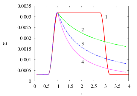
Figure 2: The initial surface density profile for $\alpha_{\mathrm{\Sigma}}$ ranging from $0.0$ to $-1.5$ (outward migration case).

2.3 Simulation setup

In the simulations we adopt non-dimensional units, where the sum of star and planet mass $M_{\mathrm{S}}+M_{\mathrm{P}}$ represents the unit of mass. The time unit and the length unit are chosen to make the gravitational constant $G=1$. This makes the orbital period of Keplerian rotation at a radius $a=1$ around a unit mass body equal to $2\pi$. However, when it is necessary to convert quantities into physical units, we use a Solar-mass protostar $M_{\mathrm{S}}=M_{\astrosun}$, a Jupiter-mass protoplanet $M_{\mathrm{P}}=M_{\jupiter}$, and a length unit of $5.2$ AU. This makes the time unit equal to $11.8/2\pi$ years.

In all the simulations the grid extends from $-4.0$ to $4.0$ in both directions around the star and planet mass centre. This corresponds to a disc region with a physical radius of $20.8$ AU.

2.3.1 Initial conditions

The initial surface density $\Sigma$ profile is given by a modified power law:

$$\Sigma=\psi(r_{\mathrm{c}})\Sigma_{\mathrm{0}}(r_{\mathrm{c}}/r_{0})^{\alpha_{\mathrm{\Sigma}}},$$ (18)

where $r_{\mathrm{c}}=|\mn@boldsymbol{r}-\mn@boldsymbol{r}_{\mathrm{C}}|$ is the distance to the mass centre of the planet-star system, $r_{0}$ is a unit distance, and $\psi$ is a function that allows introducing a sharp edges in the disc (see Fig. 2).

We characterize the disc mass by the disc to the primary mass ratio

$$\mu_{\mathrm{D}}={{\Sigma(r_{0})\pi r_{0}^{2}}\over{M_{\mathrm{S}}}}={{\Sigma_{\mathrm{0}}\pi r_{0}^{2}}\over{M_{\mathrm{S}}}}.$$ (19)

In the simulations $\mu_{\mathrm{D}}$ ranges from $0.001$ to $0.01$. For the Minimum Mass Solar Nebula (MMSN) $\mu_{\mathrm{D}}=0.00144$ (for $\alpha_{\mathrm{\Sigma}}=-3/2$). We investigate different density profiles by changing $\alpha_{\mathrm{\Sigma}}$ from $-1.5$ to $0.0$.

Since we focus on type III migration only and do not analyse the problem of orbital stability inside a gap, we do not introduce the planet smoothly nor keep it on a constant orbit for the time needed to create a gap. For most cases with $\alpha_{\mathrm{\Sigma}}<0.0$ the density gradient given by the initial profile is sufficient to start rapid inward migration. In the case of outward migration we start migration by introducing an additional density jump at the planet’s position.

The planet mass is taken to be $M_{\mathrm{P}}/M_{\mathrm{S}}=0.001$ (i.e. one Jupiter mass, $M_{\jupiter}$, for a one-solar-mass star). The planet starts on a circular orbit of semi-major axis equal $3.0$ and $0.8$ for the inward and outward migration case respectively.

The aspect ratio for the disc with respect to the star is fixed at $h_{\mathrm{s}}=0.05$, whereas the circumplanetary disc aspect ratio $h_{\mathrm{p}}$ is taken from the range $0.2$ to $0.6$.

The smoothing length of the stellar potential, $r_{\mathrm{soft}}$, is taken to be $0.5$. Unless otherwise noted, for the planet the standard value is $0.33R_{\mathrm{H}}$, where $R_{\mathrm{H}}=a{[M_{\mathrm{P}}/(3M_{\mathrm{S}})]}^{(1/3)}$, the Hill radius. The corresponding size of the envelope $r_{\mathrm{env}}$ in Eq. (13) is set to $r_{\mathrm{soft}}$ or $0.5R_{\mathrm{H}}$.

If accretion onto the planet is included, we use an accretion time-scale $\tau_{\mathrm{acc}}=10\pi$ and $r_{\mathrm{acc}}=0.5r_{\mathrm{soft}}$.

2.3.2 Boundary conditions

To stop reflections off the boundary, we use an outflow-inflow boundary condition with a so-called killing wave zone. This zone extends from radius $3.65$ to $3.9$. In this region the solution of the Euler equations for $X$ ($X$ stands for the surface density or the velocity) is changed after each time-step by

$$\Delta X={{dt}\over{\tau_{\mathrm{d}}}}(X-X_{\mathrm{0}})\phi(r),$$ (20)

where $X_{\mathrm{0}}$ is the initial condition (disc in sub-Keplerian rotation), $\tau_{\mathrm{d}}$ is the damping time-scale, and $\phi(r)$ is a function increasing from $0$ at the inner boundary of the killing wave zone to $1$ at the outer boundary of the killing wave zone. Outside the radius $3.9$ the solution $X$ is replaced by $X_{\mathrm{0}}$. In our simulations we use $\tau_{\mathrm{d}}=18$.

On our Cartesian grid the disc cannot be treated as an isolated system and some mass and angular momentum flow through the boundary is unavoidable. However, the losses are usually relatively small.

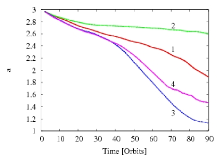
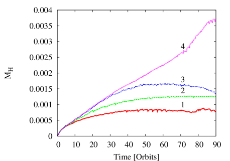
Figure 3: Convergence test for the inward migrating Jupiter. The left panel shows the time evolution of the planet’s semi-major axis $a$, the right panel the mass of the gas inside a Hill sphere $M_{H}$. Curves 1 and 2 correspond to simulations with 4 and 5 levels of refinement and $r_{\mathrm{env}}=0$ (planet acceleration is not added to the gas acceleration); curves 3 and 4 correspond to simulations with 4 and 5 level of refinement and $r_{\mathrm{env}}=0.5R_{\mathrm{H}}$. The time unit is the orbital period of the body circulating at $a=1$. The planet mass $M_{\mathrm{P}}=0.001$.

3 Description of the numerical method

3.1 Code

We adopted the FLASH hydro code version 2.3 written by the FLASH Code Group from the Centre for Astrophysical Thermonuclear Flashes at the University of Chicago in 1997.

FLASH is a modular, adaptive-mesh, parallel simulation code capable of handling general compressible flow problems. It is designed to allow users to configure initial and boundary conditions, change algorithms, and add new physics modules. It uses the PARAMESH library (MacNeice et al., 2000) to manage a block-structured adaptive mesh, placing resolution elements only where they are needed most. PARAMESH consists of a set of subroutines which handle refinement/derefinement, distribution of work to processors, guard cell filling, and flux conservation. It also uses the Message-Passing Interface (MPI) library to achieve portability and scalability on parallel computers. For our purpose, the code is used in the pure hydrodynamical mode in two dimensions, and the adaptive mesh is used to achieve high resolution around the planet (see Sect. 3.2).

Euler’s equations are solved using a directionally split version of the Piecewise-Parabolic Method (PPM, Colella & Woodward 1984). It represents the flow variables inside the cell with piecewise parabolic functions. This method is considerably more accurate and efficient than most formally second-order algorithms.

To solve the equations of motion for the star and the planet we use a 4-th order Runge-Kutta method. To keep the second order accuracy in time PPM needs information about the gravitational field from the beginning and the end of the time-step. Therefore we perform the integration of the planet’s orbit in two steps. First we integrate using the force exerted by gas taken from the previous hydro-step, This provides PPM with the approximate position of the planet at the end of the current time-step. Second, after updating the hydrodynamic quantities, we correct the planet position using a linear interpolation between the old and new values of acceleration.

3.2 Mesh and grid structure

High resolution is needed to calculate accurately the gas flow in the planet’s vicinity. For this purpose we use the Adaptive Mesh Refinement (AMR) module included in FLASH. AMR allows us to change the grid structure during the simulation, and gives the possibility for the refined region to follow the planet’s motion. The resolution is increased by a factor of 2 between refinement levels. Our simulations use a lowest resolution mesh of $800$ cells in each direction, and a square region around the planet is refined. The maximal cell size in the disc (lowest level of refinement) is about 1% of the smallest value of the planet’s semi-major axis. The cell size close to planet is at least 1.8% of Hill sphere radius (corresponding to 4 levels of refinement).

We use a Cartesian grid for our calculations. This choice was made because the more usual cylindrical (co-rotating) grid geometry has few benefits for the case of a rapidly migrating planet, and also suffers from variable (physical) resolution with radius. However, this does not mean that a Cartesian grid is problem free. The most important problem is the diffusivity of the code visible in de Val-Borro et al. (2006), however the time-scale of this process is relatively long and does not influence the rapid migration. It is discussed in Appendix A.

3.3 Multi-level time integration

In order to reduce the computational time we extended FLASH with the option of different time-steps for different refinement levels. The algorithm used is very similar to nested-grid technique presented in D’Angelo et al. (2002). Coarser blocks can use longer time-steps than finer blocks, but all blocks at a given resolution have to use the same time-step. In this case a time-step is a monotonic function of the grid resolution (in FLASH all time-steps have to be power of 2 multiples of the time-step being used on the finest block). This resolution dependent time-step can save a lot of computer time, but perhaps more importantly reduces the numerical diffusion in blocks at coarser refinement levels, which need a fewer number of time-steps to calculate a given evolution time.

4 Numerical convergence

The problem of type III migration is numerically challenging since we have to deal with the complex evolution of the co-orbital flow in a partially gap opening regime, close to the planet. Clearly one can expect the results to depend on the disk model close to the planet, and in this section we investigate how the convergence behaviour (dependence on resolution) depends on our choices for the correction for self-gravity ($r_{\mathrm{env}}$), circumplanetary disc aspect ratio ($h_{\mathrm{p}}$), and gravitational softening ($r_{\mathrm{soft}}$). Here we discuss the inward migration case only, but the conclusion are valid for the outward directed migration too.

D’Angelo et al. (2005) showed that it is hard to achieve numerical convergence for these types of flows. They found the migration to be highly dependent on the torque calculation prescription, and on the mesh resolution (see their Fig. 8 and 9). We can qualitatively reproduce their results when using EOS1, and for $r_{\mathrm{env}}=0$ and $M^{*}_{\mathrm{P}}=M_{\mathrm{P}}$ (Eq. 13), see curves 1 and 2 in Fig. 3. In this case higher resolution allows more mass to accumulate in the planet’s vicinity, and the lack of any self-gravity allows this mass to increase the planet’s inertia, slowing down its migration.

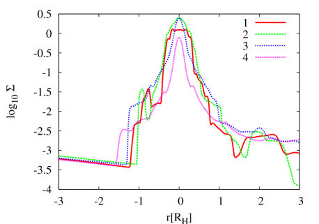
Figure 4: Surface-density radial cut through the Roche lobe at the planet position for different temperature profiles. Curve 1 corresponds to EOS1 (Eq. (10); curves 2, 3 and 4 to EOS2 (Eq. (11) with $h_{\mathrm{p}}$ equal $0.2$, $0.3$ and $0.4$ respectively.

4.1 Correction for gas self-gravity

As explained in Sect. 2.1.2 neglecting self-gravity is likely to be one cause of this bad convergence behaviour. To explore this further we use the correction for self-gravity described in Sect. 2.1.2. The key parameter of this correction is $r_{\mathrm{env}}$, the size of the region where the gas is dynamically connected to the planet. To establish its value, we performed a series of simulations with different resolutions (3, 4, and 5 refinement levels) and different values of $r_{\mathrm{env}}$: $0.0$ (no correction), $r_{\mathrm{soft}}$ (the smoothing length for gravity) and $0.5R_{\mathrm{H}}$. The last value is bigger than the estimated radius of the circumplanetary disc. From the simulations we know that the circumplanetary disc extends up $(0.3-0.4)R_{\mathrm{H}}$ (see Fig. 5). We can expect $r_{\mathrm{env}}$ to be bigger than the radius of the circumplanetary disc, since Eq. (13) does not define a sharp edge to the planet’s envelope. Some of the results of these tests are presented in Fig. 3. In these simulations we used a constant $M^{*}_{\mathrm{P}}=M_{\mathrm{P}}$.

We see that the correction reduces the ‘additional inertia’ and increases the migration rate, even though the mass of the gas accumulated in the Hill sphere increases significantly (right panel). For $r_{\mathrm{env}}=r_{\mathrm{soft}}$ the correction region is smaller than the real size of the planet envelope, and we find results similar to curves 1 and 2. The convergence is much better for $r_{\mathrm{env}}=0.5R_{\mathrm{H}}$ (curves 3 and 4), but even there we have not reached complete convergence with 5 refinement levels. This is caused by the mass accumulation in the circumplanetary disc. Comparing the simulations with 4 and 5 refinement levels (curves 3 and 4 respectively) we can see that the planet migrates faster after the mass accumulation in the circumplanetary disc stops. As the amount of mass accumulation depends on the assumed thermal structure of the circumplanetary disc (here taken to follow EOS1), we will explore this point more in the next section.

One may consider excluding the Roche lobe interior from the torque calculation as another solution to the artificial inertia problem (Masset & Papaloizou, 2003). However, the gas flow in the planet vicinity is very variable and it is impossible to define a single cutting radius to remove the region dynamically connected to the planet from the torque calculation and at the same time keep all the flow-lines that belong to the corotational flow. Moreover, in the case of the fast migration, the interior of the Roche lobe is not separated from the corotational flow and we cannot neglect the gas inflow into the circumplanetary disc (Fig. 5).

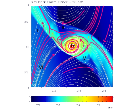
Figure 5: The flow in the planet’s proximity for the rapid inward migration. In this case the flow symmetry is broken and the big ammount of the mass is accumulated in the planet’s proximity. The plot shows the surface density distribution and the flow lines in the frame co-moving with the planet and covers a square region of the size of $4R_{\mathrm{H}}$. The colour scale is logarithmic. The pink lines show the approximate borders of the different regions in the disc: inner disc I, outer disc II, horseshoe region III, circumplanetary disc IV, co-orbital flow transferring the gas from the inner to the outer disc V and the gas stream entering the circumplanetary disc VI. The arrows show the direction of the flow.

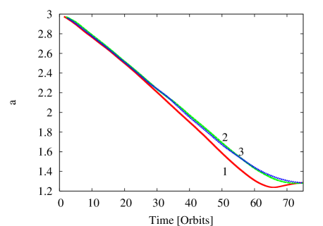
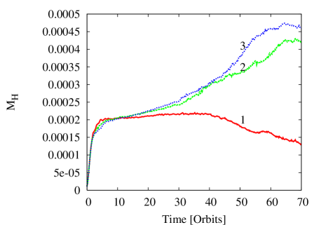
Figure 6: Convergence test for the inward migrating Jupiter with the disk aspect ratio $h_{\mathrm{p}}=0.4$. The left panel shows the time evolution of the planet’s semi-major axis $a$, the right panel the mass of the gas inside a Hill sphere $M_{H}$. Curves 1, 2 and 3 correspond to 3, 4 and 5 levels of refinement. The planet mass $M_{\mathrm{P}}=0.001$.

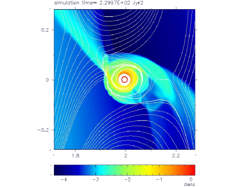
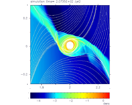
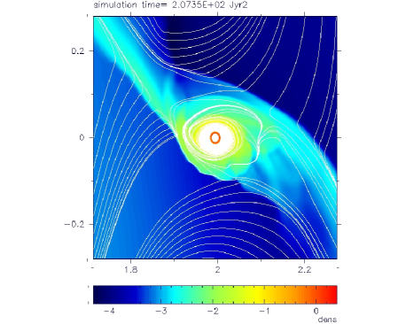
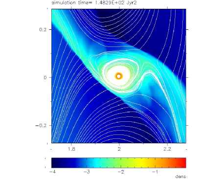
Figure 7: Surface density and the flow lines in the planet’s vicinity for an inward migrating Jupiter. Different plots correspond to different temperature profiles. Upper-left: EOS1 (no dependence on the planet’s position). Upper-right, lower-left and lower-right: EOS2 with $h_{\mathrm{p}}$ is equal $0.2$ , $0.3$ and $0.4$ respectively. The plotted domain is a square region of the size of $4R_{\mathrm{H}}$. The colour scale is logarithmic.

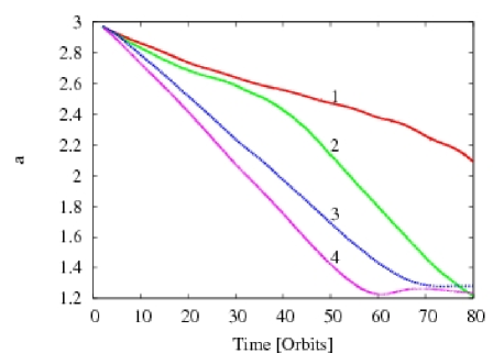
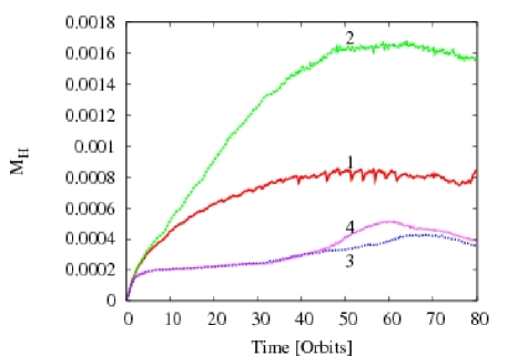
Figure 8: The planet’s orbital evolution for four discussed models: the simplest model without any corrections (curve 1), the model with correction of the gas acceleration (curve 2), the model with changed temperature profile (curve 3) and the final model with with the correction to the gas acceleration applied and the temperature rising in the planet vicinity (curve 4). The left panel shows the time evolution of the planet’s semi-major axis $a$, the right panel the mass of the gas inside a Hill sphere $M_{H}$. The planet mass is $M_{\mathrm{P}}=0.001$.

4.2 Temperature profile in the circumplanetary disc

As explained in Sect. 2.1.1, the use of EOS1 imposes a very thin circumplanetary disc. In such a thin disc waves can freely propagate and the shocks in the circumplanetary disc can end very close to the planet (see Fig. 4 curve 1). Such a strong shocks modify the flow inside the Roche lobe, redirecting the gas to the planet’s proximity. In the case of a planet on a constant orbit, this configuration does not cause any serious problems, since the co-orbital flow is weak and the gas inflow into the circumplanetary disc is limited. This changes for a migrating planet. In this case the inflow is potentially much larger since the planet moves into previously undisturbed disk regions. In fact, mass is often seen accumulating in the circumplanetary disc.

The flow structure of the gas in the planet’s proximity for the rapid inward migrating planet is presented in Fig. 5. On the plot we indicate the four important regions: the inner disc I, the outer disc II, co-orbital region III and the circumplanetary disc IV. For slow (type II) migration the structure of the shocks in the circumplanetary disc and the flow pattern in the Hill sphere is almost symmetric, but for the rapidly migrating planet the flow symmetry is broken. The spiral shocks in the circumplanetary disc are very time dependent and are frequently replaced by a one-arm spiral. It is caused by a strong mass inflow into the circumplanetary disc. The horseshoe region shrinks to a single tadpole-like region and a strong co-orbital flow (marked V and VI) develops. The co-orbital flow interacts with the bow shocks and finally is divided into a flow transferring matter from the inner disc into the outer disc and a stream entering the Roche lobe and accumulating in the circumplanetary disc.

Due to the strong co-orbital flow a significant amount of material is moved into the Roche lobe and starts interacting with the shocks originating in the circumplanetary disc. Since the disc aspect ratio $h$ decreases with decreasing distance to the planet, the shocks become stronger and the material moves along the shock directly to the central density spike (see curve 1 on Fig. 4). The radial size of this spike is given by gravitational softening $r_{\mathrm{soft}}$, since at this position $h$ grows and the shocks disappear. Inside this region (about $0.6r_{\mathrm{soft}}$) gas moves on circular orbits. When using EOS1 any amount of material can be added to this disc, since we neglect self-gravity and the gas does not heat up during compression. As a result the mass of the circumplanetary disc is only limited by the grid resolution and the value of $r_{\mathrm{soft}}$.

This is the cause of the failing numerical convergence for the runs with $r_{\mathrm{env}}=0.5R_{\mathrm{H}}$ described in the previous section. From Fig. 3 we see that the migration rate for the simulation with 4 refinement levels (curve 3) increases after the inflow into the circumplanetary disk stops at about $40$ orbits. This happens because gas moved from the inner to the outer disc exchanges with the planet twice as much angular momentum as the ‘accreted’ gas.

To address this problem we replace EOS1 with EOS2. The latter maintains a constant disc aspect ratio in the circumplanetary disc and keeps $h$ independent of the gravitational softening. To test the effects of this different equation of state, we performed simulations with different aspect ratios of the circumplanetary disc ($h_{\mathrm{p}}$ equal 0.2, 0.3 and 0.4) at different resolutions (3, 4 and 5 refinement levels), while neglecting our self-gravity correction ($r_{\mathrm{env}}=0$) and keeping the planet mass constant at $M_{\mathrm{P}}$ during the whole simulation.

We find that the model with $h_{\mathrm{p}}=0.2$ gives no improvement over the EOS1 results, the case with $h_{\mathrm{p}}=0.3$ gives some, but only for $h_{\mathrm{p}}=0.4$ numerical convergence for 5 refinement levels was achieved. These results can be understood by studying the density profile near the planet (Fig. 4) and density and flow patterns (Fig. 7). The $h_{\mathrm{p}}=0.2$ case gives a profile very similar to EOS1. The model with $h_{\mathrm{p}}=0.3$ results in a somewhat smoother profile, but only for $h_{\mathrm{p}}=0.4$ the density profile is smooth enough for the shocks to become unimportant, and the gas inflow into the circumplanetary disc is stopped, resulting in a lower mass inside the Roche lobe. The planet’s orbital evolution and the mass of the Hill sphere content for the $h_{\mathrm{p}}=0.4$ simulation at different refinement levels are shown in Fig. 6.

These results seem to indicate that the change of temperature profile alone is sufficient for achieving numerical convergence, even if we do not apply any corrections for self-gravity. The reason for this is the smoother density distribution and the lower mass of the gas in the circumplanetary disc. The ‘artificial inertia’ effects are particularly strong when the mass of the circumplanetary disk is high, and its density profile strongly peaked. In this case any small discrepancy between the disc centre and planet position results in strong, high frequency oscillations of all orbit parameters..

However, even for the changed temperature profile, some ‘artificial inertia’ effects remain. To illustrate this we compare the planet’s orbital evolution for four different models in Fig. 8. Model 1 is the simplest model (without any self-gravity correction and with EOS1), model 2 uses the self-gravity correction ($r_{\mathrm{env}}=0.5R_{\mathrm{H}}$), model 3 employs EOS2 ($h_{\mathrm{p}}=0.4$) but no self-gravity correction, and model 4 applies both ($r_{\mathrm{env}}=0.5R_{\mathrm{H}}$ and $h_{\mathrm{p}}=0.4$). We see that models 2, 3 and 4 show a higher migration rate than model 1. For model 2 there is a visible kink at $45$ orbits, which is the moment when the limiting mass of the circumplanetary disc is reached. This kink is invisible for model 4, since the ‘accreted mass’ is an order of magnitude smaller, and this mass is already reached after the few first orbits. Comparing models 3 and 4 we see that the latter has a larger migration rate than the third model, implying that the change of the temperature profile does not remove the effects of ‘artificial inertia’ completely. We hence should consider both mechanisms to be equally important.

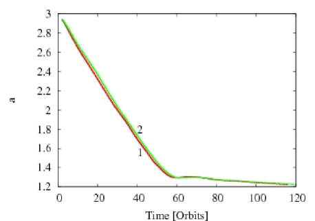
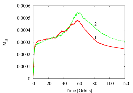
Figure 9: The planet orbital evolution for different smoothing lengths of the planet’s gravitational field for $h_{\mathrm{p}}=0.4$. The time evolution of the planet’s semi-major axis $a$ (left panel) and the mass of the gas inside a Hill sphere $M_{H}$ (right panel) are plotted. The planet mass $M_{\mathrm{P}}=0.001$. Curves 1 and 2 correspond to $r_{\mathrm{soft}}$ equal $0.0208$ and $0.3R_{\mathrm{H}}$ respectively.

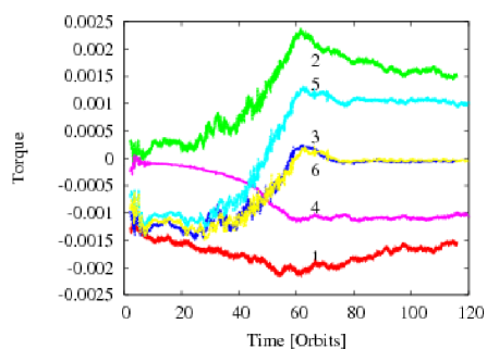
Figure 10: The torque exerted by the gas on the planet for simulations with different smoothing length of the planet gravitational field $r_{\mathrm{soft}}$ equal $0.0208$ (curves 1, 2 and 3) and $0.3R_{\mathrm{H}}$ (curves 4, 5 and 6). The torque was calculated separately for the interior of the planet’s gravitational softening $r_{\mathrm{p}}<r_{\mathrm{soft}}$ (curves 1 and 4) and the rest of the Roche sphere $r_{\mathrm{soft}}<r_{\mathrm{p}}<R_{\mathrm{H}}$ (curves 2 and 5), where $r_{\mathrm{p}}$ is the d istance to the planet. The curves 3 and 6 give the torque from the whole Hill sphere $\Gamma_{\mathrm{RL}}$ (the sum of the curves 1, 2 and 4, 5 respectively).

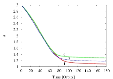
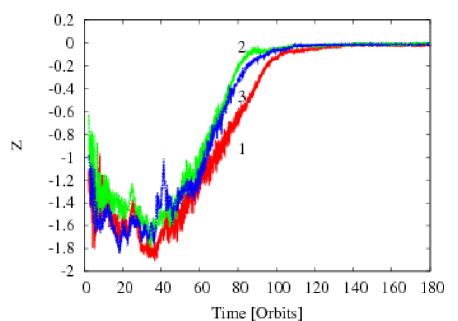
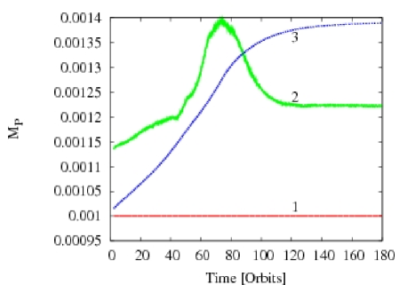
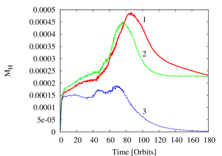
Figure 11: Results of the simulations for the varying planet’s mass and $h_{\mathrm{p}}=0.4$. Curve 1 corresponds to the model with the constant planet’s mass $M_{\mathrm{P}}=0.001$. Curve 2 shows the simulation with the effective mass of the planet augmented with the mass within the planet’s smoothing length ($\widetilde{M}_{\mathrm{P}}$). Curve 3 presents the model with an accreting planet. Upper left and upper right panels show the orbital evolution and the non-dimensional migration rate $Z$ respectively. The planet mass and the mass of the gas inside a Hill sphere are presented on the lower left and lower right panels. During the first $70$ orbits (fast migration limit $|Z|>1$) all systems evolve almost exactly the same way. Although in the fast migration regime the migration rate $\dot{a}$ is identical in simulations 1 and 2 and the differences for the accreting model are small, $Z$ differs slightly, since $\dot{a}_{\mathrm{f}}$ depends on the planet mass. The simulations start to differ after reaching the slow migration limit.

5 Torque calculation and effective planet mass

In the previous section we discussed the modifications of the disc model that allow to achieve the numerical convergence. In this chapter we will concentrate on the calculation of the torque inside the Hill sphere, and the models with the varying planet mass. Especially we will focus on the dependence of the migration on the choice of $M_{\mathrm{P}}^{*}$. We will discuss it for the inward and outward migration case separately.

5.1 Inward migration case

5.1.1 Gravitational softening

When including all material inside the Roche lobe in the calculation of the torque, the value for the gravitational softening $r_{\mathrm{soft}}$ can play an important role, even though increasing the value of the circumplanetary disc aspect ratio $h_{\mathrm{p}}$ should make $\dot{a}$ less dependent on $r_{\mathrm{soft}}$. Indeed we find that for $h_{\mathrm{p}}\geq 0.4$ the migration behaviour does not depend on $r_{\mathrm{soft}}$. The results of the runs with $h_{\mathrm{p}}=0.4$ and $r_{\mathrm{soft}}$ equal $0.0208$ and $0.3R_{\mathrm{H}}$ are presented in Fig. 9. In the first case $r_{\mathrm{soft}}$ is constant during the simulation and its value in $R_{\mathrm{H}}$ units is ranging from $0.1R_{\mathrm{H}}$ (initial value) up to about $0.25R_{\mathrm{H}}$. In both simulations we used $M^{*}_{\mathrm{P}}=M_{\mathrm{P}}$. The first and the second plot show the planet orbital evolution and the mass of the gas inside a Hill sphere. The orbital evolution is independent on the size of smoothing lengths of the planet’s gravitational field, however a larger $r_{\mathrm{soft}}$ allows the planet to accumulate larger amounts of material.

Above we have argued against excluding any part of the disc in the torque calculation. The results in this section allow this to be illustrated better. Figure 10 presents the torque exerted on the planet by the gas contained within the Hill sphere. Curves 3 and 6 show the torque from the entire Hill sphere $\Gamma_{\mathrm{RL}}$. We divided this torque into two parts, namely the contribution from $r_{\mathrm{p}}<r_{\mathrm{soft}}$ ($\Gamma_{\mathrm{soft}}$, curves 1 and 4) and the contribution from $r_{\mathrm{p}}>r_{\mathrm{soft}}$ ($\Gamma_{\mathrm{out}}$, curves 2 and 5), where $r_{\mathrm{p}}$ is the distance to the planet. The two set of curves (1, 2, 3) and (4, 5, 6) correspond to $r_{\mathrm{soft}}$ equal $0.0208$ and $0.3R_{\mathrm{H}}$ respectively.

$\Gamma_{\mathrm{RL}}$ is driving the migration during the fast migration phase (first $60$ orbits) and drops in the slow, type II like migration phase. As we saw before, it is almost independent on $r_{\mathrm{soft}}$. However, the partial torques $\Gamma_{\mathrm{soft}}$ and $\Gamma_{\mathrm{out}}$ are varying strongly between the two choices for $r_{\mathrm{soft}}$. During the fast migration phase even the sign of $\Gamma_{\mathrm{out}}$ depends on $r_{\mathrm{soft}}$. During the slow phase the two choices for the softening/cutting radius both give a positive $\Gamma_{\mathrm{out}}$, but its value increases with decreasing $r_{\mathrm{soft}}$, consistent with what was found by D’Angelo et al. (2002). $\Gamma_{\mathrm{soft}}$ has a similar but negative value and thus $\Gamma_{\mathrm{RL}}$ is close to zero, independent of the value of $r_{\mathrm{soft}}$.

This illustrates the point made before: the interior of the Roche lobe is a complicated and variable dynamical system, and it is difficult to define a simple spherical region of radius $r_{\mathrm{cut}}$, that dynamically belongs to the planet and could be neglected in the torque calculation. Any fast migration calculation would be very sensitive to the choice of $r_{\mathrm{cut}}$ (D’Angelo et al., 2005), and a wrong choice can give systematic errors in the torque calculation. It is therefore better to include all of the torques, even though this implies dealing with the region very close to the planet.

5.1.2 Mass accumulation in the planet’s vicinity

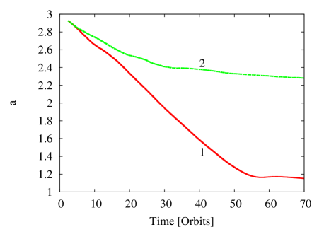
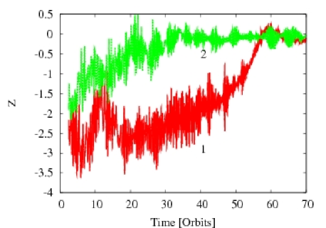
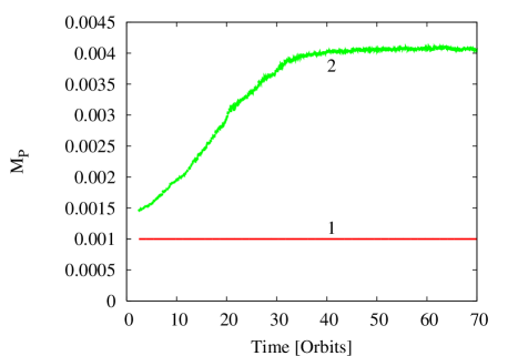
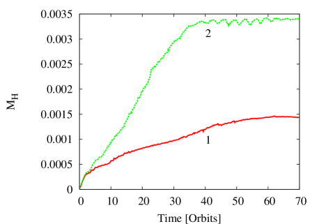
Figure 12: Results of the simulations of inward migrating planet with the varying planet’s mass for $h_{\mathrm{p}}=0.3$. Curve 1 corresponds to the model with the constant planet’s mass $M_{\mathrm{P}}=0.001$. Curve 2 shows the simulation with the effective planet mass increased by the mass within the planet’s smoothing length. Upper left and upper right panels show the orbital evolution and the non-dimensional migration rate $Z$ for the inward migrating planets respectively. The planet mass and the mass of the gas inside a Hill sphere are presented on the lower left and lower right panels.

Up to this point we studied models with a constant planet mass, neglecting the gravitational interaction of the planet’s envelope with the whole disc. However, the mass of gas accumulating in the planet’s vicinity in the case of constant $h_{\mathrm{p}}=0.4$ is comparable to the initial planet mass and can influence the orbital evolution. In this section we present models where we vary the planet’s mass.

To test the dependence of the planet’s orbital evolution on a varying planet mass we performed three simulations. In the first one the effective planet mass is constant during the whole simulation $M^{*}_{\mathrm{P}}=M_{\mathrm{P}}=0.001$, similar to the models presented above. In the second model the planet mass was replaced with all of the mass within the smoothing length $r_{\mathrm{soft}}$ around the planet ($M^{*}_{\mathrm{P}}=\widetilde{M}_{\mathrm{P}}$). In the last model we studied the planet growth through gas accretion, i.e. removing gas from the planet’s environment and adding its mass and momentum to the planet (see Sect 2.1.3).

The results are presented in Fig. 11. Curves 1 and 2 correspond to the constant mass and the $\widetilde{M}_{\mathrm{P}}$ case respectively. Curve 3 presents the accreting model. The upper left and upper right panels show the orbital evolution and the non-dimensional migration rate $Z$ (see below). The planet mass and the mass of the gas inside a Hill sphere are presented on the lower left and lower right panels.

The non-dimensional migration rate $Z$ is defined as the ratio of the migration rate ${\dot{a}}$ and the so-called fast migration speed ${\dot{a}_{\mathrm{f}}}$

$$Z={{\dot{a}}\over{\dot{a}_{\mathrm{f}}}},$$ (21)

where $\dot{a}_{\mathrm{f}}$ is given by the ratio of the half width of the horseshoe region $x_{\mathrm{s}}$ and the libration time-scale $T_{\mathrm{lib}}$. In a Keplerian disc $\dot{a}_{\mathrm{f}}$ equals (Artymowicz & Peplinski 2007, Papaloizou et al. 2007)

$$\dot{a}_{\mathrm{f}}={{3x_{\mathrm{s}}^{2}\Omega}\over{8\pi a}},$$ (22)

where $x_{\mathrm{s}}$ is estimated to be about $2.5$ Hill sphere radii. We can divide the type III migration into a fast, $|Z|>1$, and a slow, $|Z|<1$, migration regime. Type II-like migration phase corresponds to $|Z|\ll 1$. The use of $Z$ will be discussed more fully in Paper II.

During the fast migration phase (lasting for about $70$ orbits) the planet’s orbital evolution is almost independent of the planet’s mass and the mass of the circumplanetary disc. All three models show a similar evolution even though the planet’s effective mass can differ up to $40\%$ and the mass of the circumplanetary disc can differ up to $100\%$. The amount of the gas flowing into the Hill sphere (for the model with accretion the sum of the Hill sphere content and the increase of the planet’s mass) is similar too. This means that the inflow into the circumplanetary disc is a dynamical effect that mostly depends on the value of $Z$ and the initial disc surface density, and only weakly depends on the gas dynamics deep in the Roche lobe. On the other hand, it should be very sensitive to the temperature profile at the boundary of the Roche lobe. Comparing the lower left and the lower right panels of Fig. 11 we can see that most of the mass within the Roche sphere is contained within the planet’s smoothing length.

The differences between the three cases show up in the slow migration phase, where the first and the second model lose gas from the Hill sphere. The simulation with constant $M_{\mathrm{P}}$ keeps losing mass from the circumstellar disc during that entire phase, whereas in the second simulation the amount of mass within the Hill sphere converges to $1.22M_{\mathrm{P}}$. In the accreting model the amount of gas available in the planet’s vicinity and the pressure gradient are too small to cause mass loss from the circumplanetary disc. Instead the gas orbiting the planet is accreted, and in the stage of a gap creation (when the strong mass inflow into the circumplanetary disc stops) the amount of the mass inside the Hill sphere quickly decreases. At the end of the simulation the planet has reached a mass of $1.4M_{\mathrm{P}}$.

The differences in the slow migration regime ($|Z|<1$) lead to different final positions in the three cases. The reason is that $\dot{a}_{\mathrm{f}}$ depends on the planet mass. The case of a constant planet mass makes the transition to the slow phase latest, and thus achieves the smallest orbit at $a=1.1$. The difference between the $\widetilde{M}_{\mathrm{P}}$ case and the accreting planet is due to the fact that the former loses mass from the Hill sphere. This influences the migration during the end of the slow migration phase (see the difference between curves 2 and 3 between $70$ and $90$ orbits in the upper right panel of Fig. 11) and allows the accreting planet to migrate further ($a=1.2$) than the planet in the model with the effective mass increased ($a=1.3$).

As we can see, the orbital evolution differs between the fast ($|Z|>1$) and the slow ($|Z|<1$) migration limit. During the fast migration under constant $h_{\mathrm{p}}$, we can neglect details of the gas evolution deep in the circumplanetary disc, since the rate of the mass accumulation in the planet’s proximity is relatively low and the migration is driven by the outer part of the Roche lobe. However, we should keep in mind that a variation of $h_{\mathrm{p}}$ can modify the flow in the whole Roche lobe and thus can influence migration. The gas evolution in the circumplanetary disc becomes important for $|Z|\approx 1$, when the planet slows down and starts to open a gap, and the rate of the mass accumulation in the planet’s proximity increases.

To test this last dependence we performed simulations with constant planet mass (case 1 above) and with the planet’s effective mass increased by the mass within the planet’s smoothing length (case 2 above) for $h_{\mathrm{p}}$ equal $0.3$, $0.5$ and $0.6$. The results for $h_{\mathrm{p}}=0.3$ are presented in Fig. 12 (curves 1 and 2 for ${M_{\mathrm{P}}}^{*}=0.001$ and ${M_{\mathrm{P}}}^{*}=\widetilde{M}_{\mathrm{P}}$ respectively). The upper left and upper right panels show the orbital evolution and the non-dimensional migration rate $Z$, respectively. The planet mass and the mass of the gas inside a Hill sphere $M_{H}$ are presented on the lower left and lower right panels. We present here the results for $h_{\mathrm{p}}=0.3$ even though the planet’s migration is slightly dependent on $r_{\mathrm{soft}}$ for this value of the circumplanetary disc aspect ratio ($M_{H}$ grows from $0.0015$ up to $0.0022$ for $r_{\mathrm{soft}}$ changing form $0.3R_{\mathrm{H}}$ to $0.0208$, and the migration rate $\dot{a}$ differs by less than $5\%$ between both models), since it illustrates the interesting case, were the sound speed $c_{\mathrm{s}}$ at the boundary of the Roche lobe given by EOS2 is smaller than $c_{\mathrm{s}}$ given by EOS1. The model with $h_{\mathrm{p}}=0.4$ is the limiting case, where both equation EOS1 and EOS2 give the same real disc aspect ratio outside the Hill sphere (see Fig. 1). In the rest of the models EOS2 gives bigger $c_{\mathrm{s}}$ in the planet’s vicinity than EOS1.

The amount of mass accumulated in the planet’s vicinity is very sensitive to the value of $h_{\mathrm{p}}$. Unlike the model with $h_{\mathrm{p}}=0.4$, the model with $h_{\mathrm{p}}=0.3$ and ${M_{\mathrm{P}}}^{*}=M_{\mathrm{P}}$ allows the accumulation in the circumplanetary disc of an amount of mass comparable to the planet mass (about $50\%$ of $M_{\mathrm{P}}$ after $10$ orbits). In the second simulation (${M_{\mathrm{P}}}^{*}=\widetilde{M}_{\mathrm{P}}$) this mass grows faster, since the Hill radius grows with $\widetilde{M}_{\mathrm{P}}$ and the non-dimensional migration rate $|Z|$ decreases below 1, allowing a speed up of the accumulation (see Fig. 11). Finally $\widetilde{M}_{\mathrm{P}}$ reaches $4$ Jupiter masses and the planet migrates in the slow migration limit, stopping in the type II like migration at about $a=2.2$. As we can see the planet’s migration is sensitive to the rapid increase of $\widetilde{M}_{\mathrm{P}}$. The limiting case $h_{\mathrm{p}}=0.4$ was already discussed and shows the different behaviour in the slow and the fast migration limit. Increasing $h_{\mathrm{p}}$ above $0.4$ means significant decreasing $M_{\mathrm{soft}}$ and the planet’s migration becomes independent of the choice of ${M_{\mathrm{P}}}^{*}$. This allows the planet to travel faster and further. A more detailed description will be presented in Paper II.

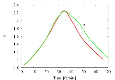
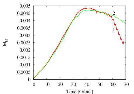
Figure 13: Orbital evolution of the outward migrating planet for different smoothing lengths of the planet’s gravitational potential. The time evolution of the planet’s semi-major axis $a$ (left panel) and the mass of the gas inside a Hill sphere $M_{H}$ (right panel) are plotted. Curves 1, 2 correspond to $r_{\mathrm{soft}}$ equal $0.0208$ and $0.3R_{\mathrm{H}}$ for $h_{\mathrm{p}}=0.4$. The planet mass $M_{\mathrm{P}}=0.001$.

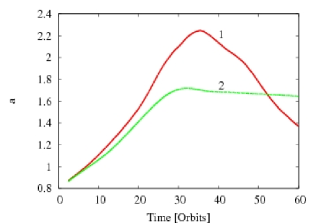
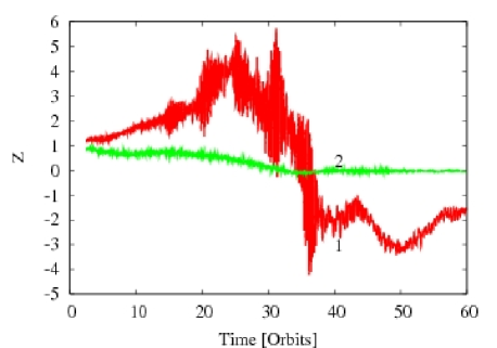
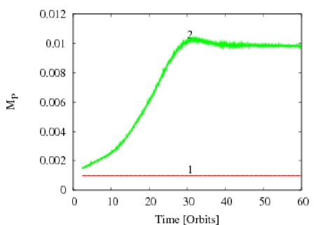
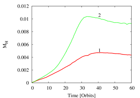
Figure 14: Results of the simulations of outward migrating planet with the varying planet’s mass. Curve 1 corresponds to the model with the constant planet’s mass $M_{\mathrm{P}}=0.001$. Curve 2 shows the simulation with the effective planet mass increased by the mass within the planet’s smoothing length. Upper left and upper right panels show the orbital evolution and the non-dimensional migration rate $Z$ for the inward migrating planets respectively. The planet mass and the mass of the gas inside a Hill sphere are presented on the lower left and lower right panels. The migration is sensitive to the value of $\widetilde{M}_{\mathrm{P}}$. In the first simulation the phases of the outward and then inward directed rapid migration are visible, but the second models shows only the first phase. Instead the planet is locked in the relatively slow migration mode at around $a=1.7$. However, during the first $20$ orbits both systems evolve in the same way, even the the mass accumulated in the planet’s proximity differ by a factor of three.

5.2 Outward migration case

Type III migration has no predefined direction and can result in both inward and outward directed migration. In the previous section we discussed the inward migration case. Most of the conclusions reached there are also valid for the outward directed migration, even though there are clear differences between the two types of simulations.

The first important difference is that the amount of mass accumulated in the circumplanetary disc is much larger in the case of outward migration, up to several times the initial planet mass. This is caused by the combination of a different gas density at the planet’s initial position, and the fact that the Roche lobe size (and the relative grid resolution) grows in the case of of outward migration. In this section we focus on the dependence of the planet’s migration on the value of the planet’s gravitational softening and the treatment of $M^{*}_{\mathrm{P}}$.

5.2.1 Gravitational softening

In Section 5.1.1 we presented the dependence of the planet’s migration on $r_{\mathrm{soft}}$ for the inward migration case. We performed similar tests for the outward migrating planet. Figure 13 shows the planet’s orbital evolution and gas mass inside the Hill sphere for two simulations with $r_{\mathrm{soft}}$ equal $0.0208$ and $0.3R_{\mathrm{H}}$ respectively. In both simulations we used $h_{\mathrm{p}}=0.4$, and $M^{*}_{\mathrm{P}}=M_{P}$.

In both cases the planet initially migrates outward but after about $35$ orbits the direction of migration suddenly changes. We find that the planet’s orbital evolution is independent of $r_{\mathrm{soft}}$ during the first $25$ orbits. When the migration speed starts to slow down, some differences between the two cases appear, and after the migration direction has reversed a clear dependence on the smoothing length becomes apparent. Still, the migration rate in both simulations differs by less than than 20% (when comparing $\dot{a}$ at a given radius rather than at given time) and the mass of the gas inside the Hill sphere remains similar up to $60$ orbits. The origin of the differences is an instability of the horseshoe region that arises for relatively high values of the migration rate. While the details of the instability are not entirely clear (streaming instability of gas with different vorticity or alternatively accelerating/decelerating migration of a planet might be involved), the net result is a decrease of the mass deficit (density contrast) of the librating disk region, which decreases the corotational torque. During the migration reversal, the numerically computed migration rate depends strongly on $r_{\mathrm{soft}}$. Therefore we limit our investigation in the case of $M^{*}_{\mathrm{P}}=M_{\mathrm{P}}$ to the outward migration phase only, which is independent of $r_{\mathrm{soft}}$.

The dependence of the torques $\Gamma_{\mathrm{soft}}$, $\Gamma_{\mathrm{out}}$ and $\Gamma_{\mathrm{RL}}$ on $r_{\mathrm{soft}}$ is similar for both the inward and the outward migration.

5.2.2 Mass accumulation in the planet’s vicinity

In Section 5.1.2 we presented models for an inward migrating planet where we used different prescriptions for $M^{*}_{\mathrm{P}}$. In the case of the outward migrating planet we performed similar simulations with $r_{\mathrm{soft}}=0.3R_{\mathrm{H}}$, $h_{\mathrm{p}}=0.4$ and $\mu_{\mathrm{D}}=0.01$. Here we only consider the cases of $M^{*}_{\mathrm{P}}=M_{\mathrm{P}}=0.001$ and $M^{*}_{\mathrm{P}}=\widetilde{M}_{\mathrm{P}}$, i.e. we do not consider the accretion case. We present the results in Fig. 14. Curves 1 and 2 correspond to the $M_{\mathrm{P}}$ and the $\widetilde{M}_{\mathrm{P}}$ case respectively. The upper left and upper right panels show the orbital evolution and the non-dimensional migration rate $Z$, the planet mass and the mass of the gas inside the Hill sphere are presented on the lower left and lower right panels.

The orbital evolution of the outward migrating planet is sensitive to the choice for $M^{*}_{\mathrm{P}}$. In the $M^{*}_{\mathrm{P}}=M_{\mathrm{P}}$ simulation the planet reaches $a=2.25$ and rapidly changes its direction of migration (as above). For the $M^{*}_{\mathrm{P}}=\widetilde{M}_{\mathrm{P}}$ case the mass accumulated in the planet’s proximity grows from an initial value of about $4.5$ ($M_{\mathrm{P}}=0.001$) up to about $10.5$ Jupiter masses. This behaviour is similar to the case of inward migrating planet with $h_{\mathrm{p}}=0.3$. The increase of $M_{\mathrm{soft}}$ causes the planet to stop around $a=1.75$ after $32$ orbits, since the disc is not massive enough to support rapid migration of such a high mass object.

The effects of neglecting the gravitational interaction between the massive planet’s envelope and the whole disc are visible on the plot of the non-dimensional migration rate $Z$. In the $M^{*}_{\mathrm{P}}=M_{\mathrm{P}}$ simulation the planet migrates in a fast migration limit with $Z>1$ and reaches $Z=4$ before it changes its direction of migration. For $M^{*}_{\mathrm{P}}=\widetilde{M}_{\mathrm{P}}$ $Z$ stays below $1$ and the planet migrates in the slow migration limit. However, the big difference in $Z$ is caused mostly by the different planet’s effective mass. During first $20$ orbits the semi-major axis $a$ differs by less than $7\%$ and the migration rate $\dot{a}$ differs at most by $25\%$. During this initial period both systems evolve in the same way, even though the mass accumulated in the planet’s proximity differs by a factor of three (about $2$ and $6$ $M_{\jupiter}$ for the two models after $20$ orbits). This is caused by the fact that for $Z>1$ the migration rate depends only weakly on the planet’s mass, and during the first $20$ orbits $Z$ is close to $Z=1$ in the $M^{*}_{\mathrm{P}}=\widetilde{M}_{\mathrm{P}}$ simulation.

This test shows that it is important to use $\widetilde{M}_{\mathrm{P}}$ when we want to study the slow migration limit of migration type III and its stopping. However, just using a constant $M_{\mathrm{P}}$ gives a correct description of the fast migration limit. For $h_{\mathrm{p}}=0.6$ the amount of mass accumulated in the circumplanetary disc and the planet’s migration become independent on the treatment of the effective mass. A more detailed description of the outward-directed type III migration will be given in Paper III.

6 Conclusions

We investigated the orbital evolution of a Jupiter-mass planet embedded in a disc and the dependence of its migration on the adopted disc model, as well as the representation of the disk-planet coupling. The calculations were performed in two dimensions in an inertial frame of reference, using a Cartesian coordinate system. We focused especially on the details of the flow in the planet’s proximity. We employed an adaptive mesh refinement code with up to 5 levels of refinement which provides high resolution in the planet’s vicinity. We conducted a careful analysis of the effects of various numerical parameters that influence the flow patterns inside the Roche lobe and the dependence on the grid resolution. Our goal was to find a disc model that allows numerical convergence to be reached and that minimises non-physical effects such as an artificial increase of the planet’s inertia. We introduced a first-order correction of the gas acceleration in the circumplanetary disc due to the gas self-gravity and a modification of the local isothermal approximation, which allows us to take into account the gravitational field of the planet when calculating the local sound speed.

For a simple disc model without these modifications to the temperature profile and the gas acceleration, we obtained results consistent with those of D’Angelo et al. (2005), depending strongly on resolution and gravitational smoothing. Convergence could only be achieved if the torques from the interior of the Hill sphere $\Gamma_{\mathrm{RL}}$ are neglected. However, the interior of the Roche lobe is important for driving rapid migration and cannot be neglected when numerically studying type III migration. Since this region is complex and dynamically variable, it is impossible to define a unique radius around the planet that would separate the planet’s sphere of influence from the disk, and thus could be neglected in the torque calculation. Therefore, one has to include all the torques from the Roche lobe, even though artificial gravitational softening must be employed on spatial scale which is much smaller than the Roche lobe. Moreover, in the case of fast migration, the interior of the Roche lobe is not separated from the corotational flow and we cannot neglect the gas inflow into the circumplanetary disc.

When including the torques from the entire Roche lobe, we achieve convergence when using the modification of the local isothermal approximation and the correction for self-gravity. Both corrections are needed and we need to use a scale height of the circumplanetary disc $h_{\mathrm{p}}\geq 0.4$ to achieve this convergence. In this case the results are insensitive to the gravitational smoothing length $r_{\mathrm{soft}}$.

However, the (converged) solution will depend on the choice for $h_{\mathrm{p}}$. It determines the flow structure inside the Roche lobe and the amount of gas accumulated in the planet’s vicinity. The latter influences the migration behaviour as the accumulation of a large mass lowers the non-dimensional migration rate $Z$. As long as $|Z|>1$, the planet migrates rapidly at a rate that is only weakly dependent on the planet’s mass and the conditions in the circumplanetary disc. If the mass accumulation forces $|Z|$ to drop below 1, migration will slow down and the planet may be locked in the disc in a mode resembling type II migration where, strictly speaking, corotational torques may still be dominant over Lindblad torques.

Our modifications of the disc model compared with previous investigations are physically justified, since the rapid accretion during migration will release potential energy and heat the gas in the planet’s environment, while self-gravity will start to play a role if the planet collects an amount of mass of order its original mass. However, our implementation of these two effects are admittedly still very crude approximations. Ideally, non-isothermal, self-gravitating models should be used to self-consistently study type III migration. For example, the assumption that the circumplanetary disk aspect ratio $h_{\mathrm{p}}$ is constant during the whole simulation is probably not realistic. However, type III migration is only weakly dependent on the mass accumulation in the fast migration limit ($|Z|>1$), so we expect variations of $h_{\mathrm{p}}$ to play an important role only in the slow migration limit ($|Z|<1$).

In summary, the migration rates of the freely migrating planet in a massive disc (satisfying the condition for rapid migration) are sensitive to the adopted disc model, especially to the treatment of the interior of the Roche lobe. The effects of heating close to the planet and self-gravity of the gas have to be taken into account to construct consistent models for type III migration. These models then show rapid migration independent of the numerical resolution used. In Papers II and III we will explore the physics of type III migration in more detail.

Appendix A Numerical diffusivity of code

Our code participated in the Hydrocode Comparison for a Disc-Planet System Project (de Val-Borro et al., 2006). In this project the results of a wide range of hydrodynamics codes were compared for the case of Jupiter- and Neptune- mass planets on a constant orbit. In this comparison differences between our Cartesian and the other (mostly) cylindrical codes were found, including a version of FLASH using a cylindrical grid.

The main difference between the Cartesian and cylindrical FLASH (denoted (FLASH-AP and FLASH-AG respectively in (de Val-Borro et al., 2006)) is a depletion of the inner disc. This leads to a deeper and broader gap, an asymmetry between the tadpole regions around the L4 and L5 Lagrangian points and a difference in the differential Lindblad torque calculation. The depletion is an effect of mass accumulation in the star’s vicinity, which takes place in a poorly resolved part of the disc (compared to the cylindrical codes). Higher resolution simulations (not discussed in de Val-Borro et al. 2006) show that this behaviour depends strongly on the grid resolution.

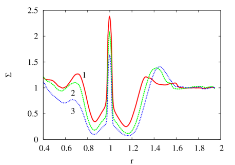
Figure 15: The normalised surface density profiles averaged azimuthally over $2\pi$ for the Jupiter-mass planet. The star’s neighbourhood is not plotted to make the plot similar to Fig. 4 in de Val-Borro et al. (2006). The curves 1, 2 and 3 correspond to 60, 150 and 300 orbits.

To further investigate this feature and its relevance for the simulations presented in the paper, we performed a test employing the typical mesh size adopted in our investigation. We used $\alpha_{\Sigma}=0$ and the Jupiter-mass planet is kept on a constant orbit with semi-major axis $a=1$. The disc extends from $-2.0$ to $2.0$ in both directions around the centre of mass and the grid has $800$ cells in both directions. The normalised surface density profile averaged azimuthally over $2\pi$ for $60$, $150$ and $300$ orbits are presented in Fig. 15 . As type III migration for Jupiter in our simulations takes about $60$ orbits on average, curve 1 is the most relevant. At the higher resolution the normalised surface density profile is almost identical to the results of the other codes in de Val-Borro et al. (2006). The depletion of the inner disk only appears at later times (curves 2 and 3). This means that the gas accumulation in the star’s vicinity is a slow process and does not play an important role for type III migration of a Jupiter-mass planet, which is anyway dominated by the co-orbital torques. Clearly for a study of the slower Type II migration, dominated by the Lindblad torques, this effect is less than beneficial.

References

- Artymowicz (2004) Artymowicz P., 2004, in Caroff L., Moon L. J., Backman D., Praton E., eds, Debris Disks and the Formation of Planets Vol. 324 of Astronomical Society of the Pacific Conference Series, Dynamics of Gaseous Disks with Planets. pp 39–+
- Artymowicz (2006) Artymowicz P., 2006, in Daflon S., Alcaniz J., Telles E., de la Reza R., eds, Graduate School in Astronomy: X Vol. 843 of American Institute of Physics Conference Series, Planetary Systems. pp 3–34
- Artymowicz & Peplinski (2007) Artymowicz P., Peplinski A., 2007, ApJ, submitted
- Boss (2001) Boss A. P., 2001, ApJ, 563, 367
- Colella & Woodward (1984) Colella P., Woodward P., 1984, J. Comput. Phys., 54, 174
- D’Angelo et al. (2005) D’Angelo G., Bate M. R., Lubow S. H., 2005, MNRAS, 358, 316
- D’Angelo et al. (2002) D’Angelo G., Henning T., Kley W., 2002, A&A, 385, 647
- D’Angelo et al. (2003) D’Angelo G., Henning T., Kley W., 2003, ApJ, 599, 548
- de Val-Borro et al. (2006) de Val-Borro M., Edgar R. G., Artymowicz P., Ciecielag P., Cresswell P., D’Angelo G., Delgado-Donate E. J., Dirksen G., Fromang S., Gawryszczak A., Klahr H., Kley W., Lyra W., Masset F., Mellema G., Nelson R. P., Paardekooper S.-J., Peplinski A., Pierens A., Plewa T., Rice K., Schafer C., Speith R., 2006, MNRAS, 370, 529
- Goldreich & Tremaine (1979) Goldreich P., Tremaine S., 1979, ApJ, 233, 857
- Goldreich & Tremaine (1980) Goldreich P., Tremaine S., 1980, ApJ, 241, 425
- Klahr & Kley (2006) Klahr H., Kley W., 2006, A&A, 445, 747
- Lin & Papaloizou (1993) Lin D. N. C., Papaloizou J. C. B., 1993, in Levy E. H., Lunine J. I., eds, Protostars and Planets III On the tidal interaction between protostellar disks and companions. pp 749–835
- Lin et al. (2000) Lin D. N. C., Papaloizou J. C. B., Terquem C., Bryden G., Ida S., 2000, Protostars and Planets IV, pp 1111–+
- MacNeice et al. (2000) MacNeice P., Olson K. M., Mobarry C., de Fainchtein R., Packer C., 2000, Computer Physics Communications, 126, 330
- Marcy et al. (2000) Marcy G. W., Cochran W. D., Mayor M., 2000, Protostars and Planets IV, pp 1285–+
- Masset et al. (2006) Masset F. S., D’Angelo G., Kley W., 2006, ApJ, 652, 730
- Masset & Papaloizou (2003) Masset F. S., Papaloizou J. C. B., 2003, ApJ, 588, 494
- Mayor & Queloz (1995) Mayor M., Queloz D., 1995, Nature, 378, 355
- Nelson & Benz (2003a) Nelson A. F., Benz W., 2003a, ApJ, 589, 556
- Nelson & Benz (2003b) Nelson A. F., Benz W., 2003b, ApJ, 589, 578
- Paardekooper & Mellema (2006) Paardekooper S.-J., Mellema G., 2006, A&A, 459, L17
- Papaloizou (2005) Papaloizou J. C. B., 2005, Celestial Mechanics and Dynamical Astronomy, 91, 33
- Papaloizou et al. (2007) Papaloizou J. C. B., Nelson R. P., Kley W., Masset F. S., Artymowicz P., 2007, in Reipurth B., Jewitt D., Keil K., eds, Protostars and Planets V Disk-Planet Interactions During Planet Formation. pp 655–668
- Peplinski et al. (2007a) Peplinski A., Artymowicz P., Mellema G., 2007a, MNRAS, submitted (Paper II)
- Peplinski et al. (2007b) Peplinski A., Artymowicz P., Mellema G., 2007b, MNRAS, in preparation (Paper III)
- Pollack et al. (1996) Pollack J. B., Hubickyj O., Bodenheimer P., Lissauer J. J., Podolak M., Greenzweig Y., 1996, Icarus, 124, 62
- Vogt et al. (2002) Vogt S. S., Butler R. P., Marcy G. W., Fischer D. A., Pourbaix D., Apps K., Laughlin G., 2002, ApJ, 568, 352
- Ward (1997) Ward W. R., 1997, Icarus, 126, 261