Bosonization approach to the mixed-valence two-channel Kondo problem

Abstract

We present in detail the bosonization-refermionization solution of the anisotropic version of the two-channel Anderson model at a particular manifold in the space of parameters of the theory, where we establish an equivalence with a Fermi-Majorana biresonant-level model. The correspondence is rigorously proved by explicitly constructing the new fermionic fields and Klein factors in terms of the original ones and showing that the commutation properties between original and new Klein factors are of semionic type. We also demonstrate that the fixed points associated with the solvable manifold are renormalization-group stable and generic, and therefore representative of the physics of the original model. The simplicity of the solution found allows for the computation of the full set of thermodynamic quantities. In particular, we compute the entropy, occupation, and magnetization of the impurity as functions of temperature, and identify the different physical energy scales. In the absence of external fields, two energy scales appear and, as the temperature goes to zero, a nontrivial residual entropy indicates that the model approaches a universal line of fixed points of non-Fermi-liquid type. An external field, even if small, introduces a third energy scale and causes the quenching of the impurity entropy to zero, taking the system to a corresponding Fermi-liquid fixed point.

I Introduction

The ideas that motivated the introduction of the two-channel Anderson model started with an attempt to describe the non-Fermi-liquid physics of the UBe₁₃ compound and other U-based heavy fermions.Cox (1987) The model can be thought of as a mixed-valence model that, in certain regimes, has the two-channel Kondo model Nozières and Blandin (1980) as its low-energy theory. In that regard, the relation between the two models is as in the case of the single-channel Kondo and Anderson models; the Anderson model captures the local-moment physics and provides a physical mechanism for moment formation, while at the same time describes also higher temperature and degenerate-level regimes for which mixed valence prevails and there are no localized moments. The study of models that capture such regimes is important, since there exist a growing number of compounds that are believed to display mixed valence [besides the large number of U-based compounds, recently, a number of new Pr-based heavy fermions were proposed as experimental candidates for the realization of quadrupolar-Kondo ground states; for instance, La-doped PrPb₃ (Ref. Kawae et al., 2006)]. Hence, improving our comprehension of the Anderson model physics is important for the phenomenological description of all these compounds.Cox and Zawadowski (1998) The peculiarity of U or Pr ions compared to the ions in other typical heavy-Fermion compounds is that, in a cubic crystal field, the $5f^{2}$ configuration of U⁺⁴ ions or the $4f^{2}$ configuration of Pr⁺³ are projected into a non-Kramers $\Gamma_{3}$ doublet with a quadrupolar moment. Fluctuations out of this state will hybridize with Kramers-degenerate states and provide a competition between magnetic and quadrupolar (i.e., flavor) moments. A minimal model in the case of the uranium compounds, that takes into account spin-orbit and crystal-field effects, leads to modeling those two states with $\Gamma_{3}$ (flavor) and $\Gamma_{6}$ (spin) doublets that hybridize with $\Gamma_{8}$ conduction electrons and give rise to a description in terms of the two-channel Anderson model.Cox and Zawadowski (1998) The situation is similar in the case of praseodymium compounds.Hotta (2005, 2006)

For the case of UBe₁₃, it was originally speculated that the $\Gamma_{3}$ doublet would constitute the lowest-energy ionic configuration. This opened the possibility of a quadrupolar route to two-channel Kondo physics, in which a local quadrupolar moment would be screened by conduction electrons whose spin degree of freedom would provide the two degenerate channels.Cox (1987) Nonlinear susceptibility measurements disfavored such scenario,Ramirez et al. (1994) however, and indicated instead the possibility of a mixed-valence state.Aliev et al. (1995) The latter was also supported by de Haas–van Alphen measurements of uranium-doped samples of ThBe₁₃.Harrison et al. (2001) The new scenario necessitates the study of the full two-channel Anderson model away from its local-moment regimes, where a low-energy Kondo-Hamiltonian description is not available. Subsequent theoretical studies of the model firmly established the persistence of local non-Fermi-liquid physics over its whole parameter regime, including at mixed valence.Schiller et al. (1998); Koga and Cox (1999); Bolech and Andrei (2002) For a contrast, one could call this the mixed-valence route to two-channel Kondo physics. In contradistinction, the quadrupolar route, –practically dismissed for uranium compounds–, recently acquired new relevance in the context of certain praseodymium compounds. Measurements on PrPb₃,Kawae et al. (2006); Onimaru et al. (2005) PrOs₄Sb₁₂,Bauer et al. (2002, 2006) and other Pr-based skutterudite compounds are consistent with the possibility of nonmagnetic ionic ground states and either onsite or offsite (antiferro)-quadrupolar fluctuations. For a summarized account of some of these experimental results, put in the context of Kondo physics, see, for instance, Ref. Maple, 2005.

In parallel, the Kondo effect became an important subject of study in the field of mesoscopics and there are many proposals and experiments for realizing two-channel Kondo systems using tunable setups such as quantum dots.Berman et al. (1999); Oreg and Goldhaber-Gordon (2003); Shah and Millis (2003); Kakashvili and Johannesson (2007); Potok et al. (2007) Experimental realizations based on the two-channel Anderson model may be more robust and allow for the observation of Kondo physics at higher temperatures, since the Kondo scale increases exponentially as the system goes into the mixed-valence regime; the Kondo physics should still be observable in quantities like the charge fluctuations encoded in the measurements of capacitance lineshapes.Bolech and Shah (2005)

Since the original work of Kondo,Kondo (1964) the study of quantum impurity models evolved rapidly. It quickly became evident that other methods going beyond perturbation theory were required in order to access the low-temperature physics of these models. The most conspicuous achievements in this front were the numerical renormalization group developed by Wilson Wilson (1975) and the Bethe ansatz solution obtained independently by Andrei and Wiegmann.Andrei (1980); Wiegmann (1980) Another important development was the identification by Toulouse Toulouse (1969); Schlottmann (1978) of a solvable line on which an anisotropic version of the model is mapped into a fermionic resonant-level model.Vigman and Finkel’shteǐn (1978) These non-perturbative techniques are required in order to study the crossover regimes and allow the unambiguous identification of the strongly coupled fixed point of the quantum impurities. Numerical renormalization group and Bethe ansatz were both applied successfully to Hamiltonians that incorporate valence fluctuation physics,Hewson (1993) but mappings like the one discovered by Toulouse remained mostly restricted to exchange models with fixed valence (cf. Ref. Kotliar and Si, 1996). In the present work, we address this missing link.Bolech and Iucci (2006a)

As compared to other non-perturbative techniques applied to quantum impurity problems,Andrei et al. (1983); Wilson (1975); Affleck (1995) bosonization –or Coulomb gas– based mappings are complementary and especially valuable in that they provide us with simple alternative ways of visualizing the physics,Giamarchi (2004) and, in particular, the different crossovers. In this paper, we examine a mapping between the anisotropic two-channel Anderson impurity model and a particularly simple biresonant-level Hamiltonian. Our work generalizes the results of the Emery-Kivelson mapping for the two-channel Kondo Hamiltonian Emery and Kivelson (1992); Fabrizio et al. (1995); Schofield (1997); Ye (1997); von Delft et al. (1998) to a more involved and descriptive model that contains, as well, the physics of charge fluctuations. After the mapping, it becomes simpler to identify the different crossover energy scales of the problem and to infer the existence of a line of non-Fermi-liquid fixed points that governs the low-energy physics.Johannesson et al. (2003, 2005) Using a renormalization group analysis, we establish the generic nature of our low-temperature results and their relevance for the original two-channel Anderson model. We show how to calculate all the dynamical and thermodynamical quantities of interest pertaining to the impurity over the full range of parameters and connect explicitly all the different temperature regimes of the system. We rederive, in a compellingly compact language, all the results obtained previously for the model using a variety of other non-perturbative techniques, Schiller et al. (1998); Bolech and Andrei (2002); Anders (2005); Bolech and Andrei (2005) and obtain a number of additional results for the situation when external fields are present and the character of the infrared fixed points is modified.

The rest of the article is organized as follows. In Sec. II, we introduce the anisotropic two-channel Anderson model, including possible external fields acting on the impurity. In Sec. III, we establish the mapping, for a set of couplings belonging to a certain manifold, onto a non-interacting Fermi-Majorana biresonant-level model. The mapping is carried out in a bosonized language and particular emphasis is put on the careful treatment of Klein factors. In Sec. IV, we perform a renormalization group analysis of the stability of the fixed points contained in the soluble manifold. In Sec. V, we identify the three crossover scales of the model and compute thermodynamic quantities in the entire temperature range and for arbitrary values of the external fields. Finally, in Sec. VI, we provide a summary of our conclusions and an outlook of the applications of the mapping to other problems involving two-channel Anderson model physics.

II The anisotropic two-channel Anderson model

We shall consider a generalized version of the two-channel Anderson model to which we add terms that break the rotation invariance in spin and flavor spaces. This is akin to the standard practice in the case of the single-channel Kondo model of considering an exchange coupling constant that acquires a different value along the $z$-axis. We denote the Hamiltonian as

$$H=H_{\text{host}}+H_{\text{imp}}+H_{\text{hyb}}+H_{\text{field}}+H_{3}~{}\text{.}$$ (1)

The first term describes the dynamics of the band electrons ($\psi_{\alpha\sigma}^{\dagger}$ where $\sigma=\uparrow,\downarrow$ and $\alpha=+,-$ correspond to the spin and flavor degrees of freedom, respectively) in the standard approximation of a linearized band dispersion around the Fermi level fixed by the normal order prescription,

$$H_{\text{host}}=\sum_{\alpha\sigma}\int dx~{}:\psi_{\alpha\sigma}^{\dagger}\left(x\right)\left(-iv_{\text{F}}\partial_{x}\right)\psi_{\alpha\sigma}\left(x\right):~{}\text{.}$$ (2)

The second and third terms contain the isolated-impurity contribution and the band-impurity hybridization, respectively,

$$H_{\text{imp}} =\varepsilon_{s}\sum_{\sigma}X_{\sigma\sigma}+\varepsilon_{f}\sum_{\alpha}X_{\bar{\alpha}\bar{\alpha}}~{}\text{,}$$ (3a)

$$H_{\text{hyb}} =V\sum_{\alpha\sigma}\left[X_{\sigma\bar{\alpha}}\psi_{\alpha\sigma}\left(0\right)+\psi_{\alpha\sigma}^{\dagger}\left(0\right)X_{\bar{\alpha}\sigma}\right]~{}\text{.}$$ (3b)

Here, we have used Hubbard-operator notation to describe the impurity degrees of freedom ($$X_{ab}=\left|a\right\rangle\left\langle b\right| a,b=\sigma,\bar{\alpha}$$ where and the bar stands for the complex-conjugate representation). As compared to slave-operator notation, the use of Hubbard operators automatically restricts the Hilbert space of the impurity to the physical one.Bolech and Andrei (2005) These first three terms constitute the standard two-channel Anderson model. The fourth term describes the coupling to external fields:

$$H_{\text{field}}=h_{s}(X_{\downarrow\downarrow}-X_{\uparrow\uparrow})+h_{f}\left(X_{\bar{+}\bar{+}}-X_{\bar{-}\bar{-}}\right)~{}\text{,}$$ (4)

where, for the sake of generality, we included two fields: one coupling to the impurity spin and the other one coupling to its flavor. Finally, the fifth term provides the generalized anisotropy and can be written as a sum over charge ($c$), spin($s$), flavor ($f$), and spin-flavor ($s\!f$) sectors (as will be seen below, these sectors arise naturally after bosonizing the model),

$$H_{3}=\sum_{\nu=c,s,f,s\!f}H_{3}^{\nu}~{}\text{,}$$ (5)

with each term taking the form of a density-density interaction between the different impurity densities with the corresponding ones from the band,

$$H_{3}^{\nu}=J_{\nu}^{3}X_{\nu}\rho_{\nu}~{}\text{,}$$ (6)

where $\rho_{\nu}\equiv\rho_{\nu}\left(x=0\right)$,

$$\rho_{\nu}\left(x\right)=\sum_{\alpha\sigma\alpha^{\prime}\sigma^{\prime}}:\psi_{\alpha\sigma}^{\dagger}\left(x\right)\Upsilon_{\alpha\sigma,\alpha^{\prime}\sigma^{\prime}}^{\nu}\psi_{\alpha^{\prime}\sigma^{\prime}}\left(x\right):$$ (7)

and

$$\Upsilon_{\alpha\sigma,\alpha^{\prime}\sigma^{\prime}}^{c} =\delta_{\alpha\alpha^{\prime}}\delta_{\sigma\sigma^{\prime}}~{}\text{,} \Upsilon_{\alpha\sigma,\alpha^{\prime}\sigma^{\prime}}^{s} =\delta_{\alpha\alpha^{\prime}}\tau^{3}{}_{\sigma\sigma^{\prime}}~{}\text{,}$$ (8a)

$$\Upsilon_{\alpha\sigma,\alpha^{\prime}\sigma^{\prime}}^{f} =\tau^{3}{}_{\alpha\alpha^{\prime}}\delta_{\sigma\sigma^{\prime}}~{}\text{,} \Upsilon_{\alpha\sigma,\alpha^{\prime}\sigma^{\prime}}^{s\!f} =\tau^{3}{}_{\alpha\alpha^{\prime}}\tau^{3}{}_{\sigma\sigma^{\prime}}~{}\text{,}$$ (8b)

(here $$\tau^{3}$$ is the third Pauli matrix). The impurity densities involved are

$$X_{s}=\sum_{\sigma}\sigma X_{\sigma\sigma}~{}\text{,}$$ (9a)

$$X_{f}=\sum_{\alpha}\alpha X_{\bar{\alpha}\bar{\alpha}}~{}\text{,}$$ (9b)

$$X_{c}=X_{s\!f}=\sum_{\sigma}X_{\sigma\sigma}-\sum_{\alpha}X_{\bar{\alpha}\bar{\alpha}}~{}\text{.}$$ (9c)

Since the impurity Hilbert space contains four states, we can define only three independent density-like operators apart from the identity; we find it convenient to define the spin-flavor density to coincide with the charge one.

III Bosonization based mapping

Bosonization is a well known technique that renders more accessible the study of 1+1 dimensional models.Haldane (1981); von Delft and Schoeller (1998); Gogolin et al. (1998); Giamarchi (2004) When combined with refermionization procedures, the bosonic language can be used to find nontrivial mappings between different fermionic models. The idea is that, many times, a mapping that results highly nonlinear in the fermionic language can be written as a simple canonical transformation in terms of the bosons.

III.1 Bosonization

We shall employ the standard bosonic representation of the fermionic fields,

$$\psi_{\alpha\sigma}\left(x\right)=\frac{1}{\sqrt{2\pi a}}F_{\alpha\sigma}e^{-i\phi_{\alpha\sigma}\left(x\right)}~{}\text{,}$$ (10)

in which $a$ is a regulator that plays the role of an inverse bandwidth and $\phi_{\alpha\sigma}$ are bosonic fields that describe the particle-hole excitations around the Fermi sea. Finally, $F_{\alpha\sigma}$ are the so called Klein factors, responsible for recovering the correct anticommutation relations among different fermionic species and necessary for describing processes in which the number of fermions changes. They act as ladder operators in the fermionic Hilbert space and commute with the $\phi$’s. Additionally, they satisfy the following algebra:

$$F_{\alpha\sigma}^{\dagger}F_{\alpha\sigma} =F_{\alpha\sigma}F_{\alpha\sigma}^{\dagger}=1~{}\text{,}$$ (11a)

$$F_{\alpha\sigma}^{\dagger}F_{\alpha^{\prime}\sigma^{\prime}} =-F_{\alpha^{\prime}\sigma^{\prime}}F_{\alpha\sigma}^{\dagger}\qquad\text{for}~{}\left(\alpha\sigma\right)\neq\left(\alpha^{\prime}\sigma^{\prime}\right)\text{,}$$ (11b)

$$F_{\alpha\sigma}F_{\alpha^{\prime}\sigma^{\prime}} =-F_{\alpha^{\prime}\sigma^{\prime}}F_{\alpha\sigma}\qquad\text{for}~{}\left(\alpha\sigma\right)\neq\left(\alpha^{\prime}\sigma^{\prime}\right)$$ (11c)

and they obey the following (anti)commutation relations with the impurity Hubbard operators:

$$\left[F_{\alpha\sigma},X_{\bar{\alpha}^{\prime}\bar{\alpha}^{\prime\prime}}\right] =\left[F_{\alpha\sigma},X_{\sigma^{\prime}\sigma^{\prime\prime}}\right]=0~{}\text{,}$$ (12a)

$$\left\{F_{\alpha\sigma},X_{\sigma^{\prime}\bar{\alpha}^{\prime}}\right\} =\left\{F_{\alpha\sigma},X_{\bar{\alpha}^{\prime}\sigma^{\prime}}\right\}=0~{}\text{.}$$ (12b)

In terms of the bosons, the Hamiltonian for the band takes the form

$$H_{\text{host}}=\frac{v_{\text{F}}}{4\pi}\sum_{\alpha\sigma}\int dx:\left(\partial_{x}\phi_{\alpha\sigma}\right)^{2}:~{}\text{.}$$ (13)

Following Emery and Kivelson, it is natural to introduce a rotated basis for the bosons ($\nu=c$, $s$, $f$, $s\!f$)

$$\phi_{\nu} =\frac{1}{2}\sum_{\alpha\sigma}\Upsilon_{\alpha\sigma,\alpha\sigma}^{\nu}\phi_{\alpha\sigma}~{}\text{, or}$$ (14)

$$\phi_{\alpha\sigma} =\frac{1}{2}\left(\phi_{c}+\sigma\phi_{s}+\alpha\phi_{f}+\alpha\sigma\phi_{s\!f}\right)~{}\text{,}$$ (15)

where $\sigma,\alpha=\pm$ when entering as multiplying factors. The form of $H_{\text{host}}$ remains the same in the new basis:

$$H_{\text{host}}=\sum_{\nu=c,s,f,s\!f}H_{0}^{\nu}\equiv\frac{v_{\text{F}}}{4\pi}\sum_{\nu=c,s,f,s\!f}\int dx:\left(\partial_{x}\phi_{\nu}\right)^{2}:~{}\text{.}$$ (16)

Notice that the Klein factors disappeared from the bosonized version of the first term, but they will enter explicitly in the hybridization term:

$$H_{\text{hyb}}=\frac{V}{\sqrt{2\pi a}}\sum_{\alpha\sigma}X_{\sigma\bar{\alpha}}F_{\alpha\sigma}e^{-i\left(\phi_{c}+\sigma\phi_{s}+\alpha\phi_{f}+\alpha\sigma\phi_{s\!f}\right)/2}+\text{h.c.}$$ (17)

Last, the terms involving only impurity operators stay unchanged and the terms involving exchange are bosonized according to the standard prescription for densities:

$$H_{3}^{\nu}=J_{\nu}X_{\nu}\rho_{\nu}=-\frac{J_{\nu}}{\pi}X_{\nu}\partial_{x}\phi_{\nu}(0)~{}\text{.}$$ (18)

The difficulty for studying this model is contained in the highly nontrivial form of the hybridization with the impurity. Therefore, the strategy is to look for a canonical transformation that simplifies this term. We define the following generic transformation $U=U_{c}U_{s}U_{f}U_{s\!f}$ with

$$U_{\nu}=e^{i\gamma_{\nu}\phi_{\nu}(0)X_{\nu}}~{}\text{.}$$ (19)

For transforming $H_{\text{hyb}}$, we first notice that $U$ commutes with the vertex operators and the Klein factors. Thus, we only need to compute expressions of the form $U_{\nu}X_{\sigma\bar{\alpha}}U_{\nu}^{\dagger}$. Using

$$\left[X_{\sigma\bar{\alpha}},X_{s}\right] =-\sigma X_{\sigma\bar{\alpha}}~{}\text{,} \left[X_{\sigma\sigma},X_{\nu}\right] =0~{}\text{,}$$ (20a)

$$\left[X_{\sigma\bar{\alpha}},X_{c}\right] =-2X_{\sigma\bar{\alpha}}~{}\text{,} \left[X_{\bar{\alpha}\bar{\alpha}},X_{\nu}\right] =0~{}\text{,}$$ (20b)

$$\left[X_{\sigma\bar{\alpha}},X_{f}\right] =\alpha X_{\sigma\bar{\alpha}}~{}\text{,}$$ (20c)

(note that the two identities on the right imply that $$H_{\text{imp}} H_{\text{field}}$$ and are not affected by the transformation), we obtain:

$$U_{s}X_{\sigma\bar{\alpha}}U_{s}^{\dagger} =X_{\sigma\bar{\alpha}}e^{\sigma i\gamma_{s}\phi_{s}}~{}\text{,}$$ (21a)

$$U_{f}X_{\sigma\bar{\alpha}}U_{f}^{\dagger} =X_{\sigma\bar{\alpha}}e^{-\alpha i\gamma_{f}\phi_{f}}~{}\text{,}$$ (21b)

$$U_{c}X_{\sigma\bar{\alpha}}U_{c}^{\dagger} =X_{\sigma\bar{\alpha}}e^{2i\gamma_{c}\phi_{c}}~{}\text{,}$$ (21c)

$$U_{s\!f}X_{\sigma\bar{\alpha}}U_{s\!f}^{\dagger} =X_{\sigma\bar{\alpha}}e^{2i\gamma_{s\!f}\phi_{s\!f}}~{}\text{.}$$ (21d)

Therefore, we can transform the hybridization Hamiltonian as $$\tilde{H}_{\text{hyb}}=UH_{\text{hyb}}U^{\dagger}$$, with

$$\tilde{H}_{\text{hyb}} =\frac{V}{\sqrt{2\pi a}}\sum_{\alpha\sigma}\left[X_{\sigma\bar{\alpha}}F_{\alpha\sigma}e^{-i(\frac{1}{2}-2\gamma_{c})\phi_{c}}e^{-i\alpha(\frac{1}{2}+\gamma_{f})\phi_{f}}\right.$$

$$\times\left.e^{-i\sigma(\frac{1}{2}-\gamma_{s})\phi_{s}}e^{-i(\frac{\alpha\sigma}{2}-2\gamma_{s\!f})\phi_{s\!f}}+\text{h.c.}\right]~{}\text{.}$$ (22)

Next, we use the freedom of choosing the particular transformation that will simplify the form that this term takes. Such a choice is given by taking $\gamma_{c}=1/4$, $\gamma_{f}=-1/2$ and $\gamma_{s}=1/2$, and thus decoupling the impurity from the corresponding sectors in the band. The transformed expression is

$$\tilde{H}_{\text{hyb}}=\frac{V}{\sqrt{2\pi a}}\left[\left(X_{\uparrow+}F_{\uparrow+}+X_{\downarrow-}F_{\downarrow-}\right)e^{-i(\frac{1}{2}-2\gamma_{s\!f})\phi_{s\!f}}\right.\\ +\left.\left(X_{\uparrow-}F_{\uparrow-}+X_{\downarrow+}F_{\downarrow+}\right)e^{-i(-\frac{1}{2}-2\gamma_{s\!f})\phi_{s\!f}}+\text{h.c.}\right]~{}\text{,}$$ (23)

(where we have omitted the bar over the values taken by the $\bar{\alpha}$ subindex). We can further simplify this term by choosing $\gamma_{s\!f}=\pm 1/4$. The two choices are equivalent and we choose $\gamma_{s\!f}=1/4$; in this way, we kill the vertex in the first term while giving the second one fermionic dimensions:

$$\tilde{H}_{\text{hyb}}=\frac{V}{\sqrt{2\pi a}}\left[\left(X_{\uparrow+}F_{\uparrow+}+X_{\downarrow-}F_{\downarrow-}\right)\right.\\ +\left.\left(X_{\uparrow-}F_{\uparrow-}+X_{\downarrow+}F_{\downarrow+}\right)e^{i\phi_{s\!f}}+\text{h.c.}\right]~{}\text{.}$$ (24)

The spin-flavor band and the impurity remain coupled, but the form of their hybridization is now much simpler. Before studying this term further, let us indicate what happens to the remaining terms in the Hamiltonian upon the same transformation:

$$U\left(H_{\text{host}}+H_{3}\right)U^{\dagger}=H_{\text{host}}\\ +\frac{1}{\pi}\sum_{\nu}(\pi v_{F}\gamma_{\nu}-J_{\nu})\partial_{x}\phi_{\nu}(0)X_{\nu}~{}\text{.}$$ (25)

We define for future reference the couplings

$$\lambda_{\nu}=\pi v_{\text{F}}\gamma_{\nu}-J_{\nu}~{}\text{,}$$ (26)

which can be set to be zero by tuning the values of $J_{\nu}\rightarrow\pi v_{\text{F}}\gamma_{\nu}$; thus rendering the model particularly simple, as it will be seen below.

III.2 Refermionization

Inspired by the classic results by Toulouse and by Emery and Kivelson in which they map the single- and the two-channel Kondo models, respectively, into different types of resonant-level models and find particular values of the anisotropy for which those resonant-level models are non-interacting and therefore exactly solvable, we find it compelling to seek a similar mapping for the two-channel Anderson model. However, while in the Kondo model the interactions between the band electrons and the impurity are exchange terms that involve only fermionic bilinears, that is not the case for the Anderson model in which the hybridization term allows for the flow of charge between the band and the impurity. This is an important difference that gives rise to a much richer parameter regime, in the case of the Anderson model, that includes not only local-moment phases but also mixed-valence ones. From the technical point of view, it becomes important to keep track of the charge transfer processes while bosonizing, which requires a proper treatment of the Klein factors.

III.2.1 New fermions

In order to find a mapping to a new fermionic model, we need to refermionize the version that was already simplified by the cal transformation just discussed. The first step is to introduce a new set of Klein factors that allow us to define new fermionic operators corresponding to the physical sectors ($c$, $s$, $f$, $s\!f$):

$$\psi_{\nu}=\frac{1}{\sqrt{2\pi a}}F_{\nu}e^{-i\phi_{\nu}}~{}\text{.}$$ (27)

The new Klein factors are defined to be ladder operators in the physical Hilbert space for the band and to obey the usual algebra given in Eqs. (11a)–(12b).

Inspecting $\tilde{H}_{\text{hyb}}$, we are led to define the new impurity operators:

$$d =F_{s\!f}\left(X_{\uparrow-}F_{\uparrow-}+X_{\downarrow+}F_{\downarrow+}\right)~{}\text{,}$$ (28a)

$$f =X_{-+}F_{f}+X_{\uparrow\downarrow}F_{s}~{}\text{.}$$ (28b)

They allow us to rewrite the hybridization term as

$$\tilde{H}_{\text{hyb}}=\frac{V}{\sqrt{2\pi a}}\left[\left(f^{\dagger}+f\right)d+d^{\dagger}\left(f^{\dagger}+f\right)\right]\\ +V\left(\psi_{s\!f}^{\dagger}d+d^{\dagger}\psi_{s\!f}\right)~{}\text{.}$$ (29)

The new form of the Hamiltonian looks compellingly simple. However, we will find that the new operators are not fermions. It can be seen that they satisfy the following relations:

$$d^{2} =d^{\dagger 2}=0~{}\text{,}$$ (30a)

$$dd^{\dagger} =X_{\uparrow\uparrow}+X_{\downarrow\downarrow}~{}\text{,}$$ (30b)

$$d^{\dagger}d =X_{++}+X_{--}$$ (30c)

and

$$f^{2} =f^{\dagger 2}=0~{}\text{,}$$ (31a)

$$ff^{\dagger} =X_{--}+X_{\uparrow\uparrow}~{}\text{,}$$ (31b)

$$f^{\dagger}f =X_{++}+X_{\downarrow\downarrow}~{}\text{.}$$ (31c)

Using the completeness relation for the impurity Hilbert space ($$X_{\uparrow\uparrow}+X_{\downarrow\downarrow}+X_{++}+X_{--}=1 d f d f$$), it is clear that both and are self-fermions (i.e., each of them independently obeys fermionic anticommutation relations with itself). We still need to verify the mixed commutation relations. It is important to stress that the relations written above can be deduced independently of any relation between old and new Klein factors. That is not the case for the relations mixing and .

III.2.2 Klein factor relations

Following the authors of Refs. von Delft et al., 1998 and Zaránd and von Delft, 2000, we have the freedom to make the following four identifications between the sets of old and new Klein factors:

$$F_{s\!f}^{\dagger}F_{s}^{\dagger} =F_{\uparrow+}^{\dagger}F_{\downarrow+}~{}\text{,}$$ (32a)

$$F_{s\!f}F_{s}^{\dagger} =F_{\uparrow-}^{\dagger}F_{\downarrow-}~{}\text{,}$$ (32b)

$$F_{s\!f}^{\dagger}F_{f}^{\dagger} =F_{\uparrow+}^{\dagger}F_{\uparrow-}~{}\text{,}$$ (32c)

$$F_{c}^{\dagger}F_{s}^{\dagger} =F_{\uparrow+}^{\dagger}F_{\uparrow-}^{\dagger}~{}\text{.}$$ (32d)

These relations are consistent with the physical constraints given by the variations in the fermionic numbers on the different sectors the Klein factors act upon, and the choice of signs serves to fix otherwise arbitrary phases. All other relations and their respective phases are now automatically fixed, for instance,

$$F_{s}^{\dagger}F_{f}^{\dagger} =F_{\uparrow+}^{\dagger}F_{\downarrow-}~{}\text{,}$$ (32e)

$$F_{s}F_{c}^{\dagger} =F_{\downarrow+}^{\dagger}F_{\downarrow-}^{\dagger}~{}\text{,}$$ (32f)

$$F_{f}^{\dagger}F_{s\!f} =F_{\downarrow+}^{\dagger}F_{\downarrow-}~{}\text{,}$$ (32g)

can be deduced using the first four relations.

We want now to explore further the relations between old and new Klein factors. For example, using Eqs. (32a) and (32b), one can derive the following expressions:

$$0= \left\{F_{\uparrow+},F_{\uparrow+}^{\dagger}F_{\downarrow+}\right\}=\left\{F_{\uparrow+},F_{s\!f}^{\dagger}F_{s}^{\dagger}\right\}$$

$$=\left[F_{\uparrow+},F_{s\!f}^{\dagger}\right]F_{s}^{\dagger}+F_{s\!f}^{\dagger}\left\{F_{\uparrow+},F_{s}^{\dagger}\right\}~{}\text{,}$$ (33a)

$$0= \left[F_{\uparrow+},F_{\uparrow-}^{\dagger}F_{\downarrow-}\right]=\left[F_{\uparrow+},F_{s\!f}F_{s}^{\dagger}\right]$$

$$=\left\{F_{\uparrow+},F_{s\!f}\right\}F_{s}^{\dagger}-F_{s\!f}\left\{F_{\uparrow+},F_{s}^{\dagger}\right\}~{}\text{.}$$ (33b)

Premultiplying these equations by $$F_{s\!f} F_{s\!f}^{\dagger}$$ and , respectively, and adding them up, one finds

$$F_{s\!f}F_{\uparrow+}F_{s\!f}^{\dagger}+F_{s\!f}^{\dagger}F_{\uparrow+}F_{s\!f}=0~{}\text{.}$$ (34)

Using the different relations in Eqs. (32a)–(32g), one can generalize this relation to a generic relation between old ($o$) and new ($n$) Klein factors:

$$F_{n}F_{o}F_{n}^{\dagger}+F_{n}^{\dagger}F_{o}F_{n}=0~{}\text{.}$$ (35)

Interestingly, such a relation is not consistent neither with commutation nor with anticommutation relations between the old and new Klein factors. This is not unexpected, since the two sets exist in different Hilbert spaces and the physical identification between the two is only through the relations among bilinears. While in Kondo-type models this poses no problems because only Klein factor bilinears enter in the Hamiltonians, this is not the case in Anderson-type models,Kotliar and Si (1996) for which we need to go beyond bilinears. Therefore, if we insist that the old and new Klein factors should obey a relation of the type

$$F_{n}F_{o}=\alpha F_{o}F_{n}~{}\text{,}$$ (36)

we find that $\alpha^{2}=-1$ must hold. Thus, only semionic commutation relations are consistent between old and new Klein factors and there is still an arbitrariness in the phase that needs to be fixed. Let us postulate

$$F_{\uparrow+}F_{c}=iF_{c}F_{\uparrow_{+}}~{}\text{;}$$ (37)

all other commutation relations can be deduced from this one and summarized as

$$F_{\sigma\alpha}F_{\nu} =i\theta_{\sigma\alpha}^{\nu}F_{\nu}F_{\sigma\alpha}~{}\text{,}$$ (38a)

$$F_{\sigma\alpha}F_{\nu}^{\dagger} =-i\theta_{\sigma\alpha}^{\nu}F_{\nu}^{\dagger}F_{\sigma\alpha}~{}\text{,}$$ (38b)

where $$\theta_{\sigma\alpha}^{c}=1 \theta_{\sigma\alpha}^{s}=\alpha \theta_{\sigma\alpha}^{f}=\sigma \theta_{\sigma\alpha}^{s\!f}=\sigma\alpha$$, , , and .

A similar procedure can be used to verify that the new Klein factors and the nondiagonal impurity Hubbard operators that enter in $H_{\text{hyb}}$ obey

$$F_{\nu}X_{\sigma\alpha}F_{\nu}^{\dagger}-F_{\nu}^{\dagger}X_{\sigma\alpha}F_{\nu}=0~{}\text{,}$$ (39)

which is consistent only with standard commutation or anticommutation relations between the operators and, on physical grounds, we take them to anticommute.

Using the semionic commutation relations between the two sets of Klein factors, it is easy to see that

$$df =ifd~{}\text{,}$$ (40a)

$$f^{\dagger}d =idf^{\dagger}~{}\text{.}$$ (40b)

Analogously, with respect to the spin-flavor band, we find

$$\psi_{s\!f}d =-id\psi_{s\!f}~{}\text{,}$$ (41a)

$$\psi_{s\!f}d^{\dagger} =id^{\dagger}\psi_{s\!f}~{}\text{,}$$ (41b)

and

$$\left[f,\psi_{s\!f}\right]=\left[f^{\dagger},\psi_{s\!f}\right]=0~{}\text{.}$$ (42)

We say that $d$ is a relative semion with respect to $f$ and $\psi_{s\!f}$, while the latter two are relative bosons.

On the other hand, the band fermions from the charge, spin and flavor sectors, do not have simple commutation relations with the new impurity operators. Those can be simplified by performing a unitary transformation of the Klein factors belonging to that subspace. Namely, we define

$$\tilde{F}_{s} =e^{-i\frac{\pi}{2}X_{s}}F_{s}~{}\text{,}$$ (43a)

$$\tilde{F}_{f} =e^{-i\frac{\pi}{2}X_{f}}F_{f}~{}\text{,}$$ (43b)

$$\tilde{F}_{c} =e^{-i\frac{\pi}{4}X_{c}}F_{c}~{}\text{.}$$ (43c)

The redefined operators in the decoupled bands are now relative fermions with $$d f$$, , and among themselves. Notice also that the Hamiltonian for the decoupled sectors is invariant under the redefinition. What remains is to simplify further the commutation relations among the spin-flavor operators and the impurity ones.

III.2.3 Jordan-Wigner procedure

The procedure we will use to simplify the commutation relations among the impurity and spin-flavor operators is inspired on the Jordan-Wigner treatment of spin chains. We have that $\psi_{s\!f}$, $d$ and $f$ are all self-fermions while the pairs $(\psi_{s\!f},d)$ and $\left(d,f\right)$ are relative semions and, finally, $(\psi_{s\!f},f)$ are relative bosons. For the sake of clarity, we will split the Jordan-Wigner transformation into two parts. In the first part, we shall change all operators into relative bosons, and in the second part, we will perform a standard Jordan Wigner transformation to turn them into relative fermions; that way the full system will be a system of fermions.

Defining

$$\tilde{d} =d~{}\text{,}$$ (44a)

$$\tilde{f} =e^{-i\pi n_{d}/2}f~{}\text{,}$$ (44b)

$$\tilde{\psi}_{s\!f} =e^{-i\pi n_{d}/2}\psi_{s\!f}~{}\text{,}$$ (44c)

(where $$n_{d}=d^{\dagger}d n_{f}=f^{\dagger}f$$ and ), we see that all operators are still self-fermions, but now their relative statistics is that of relative bosons:

$$[\tilde{d},\tilde{f}]=[\tilde{d},\tilde{\psi}_{s\!f}]=[\tilde{f},\tilde{\psi}_{s\!f}]=0~{}\text{.}$$ (45)

A set of operators that are relative bosons but all self-fermions, is what is usually called core bosons. They are equivalent to spin-1/2 spins and the usual Jordan-Wigner treatment is available to turn them into fermions. The second transformation is thus written as

$$f =\tilde{f}~{}\text{,}$$ (46a)

$$d =e^{-i\pi n_{f}}\tilde{d}~{}\text{,}$$ (46b)

$$\psi_{s\!f} =e^{-i\pi(n_{f}+n_{d})}\tilde{\psi}_{s\!f}~{}\text{,}$$ (46c)

(notice that we have redefined $$\psi_{s\!f} d f n_{f}=n_{\tilde{f}} n_{d}=n_{\tilde{d}} d f$$, and , and that and ). While the first Jordan-Wigner string was anchored at the site, the second one is anchored at the site; this is why it is physically more transparent to split the transformation into two steps.

Finally, since the different fermionic species can be ordered such that $\tilde{H}_{\text{hyb}}$ contains only nearest-neighbor hopping terms, it can be seen that the Jordan-Wigner strings will not appear explicitly in the Hamiltonian. After the double replacement, we find

$$\tilde{H}_{\text{hyb}}=V\left(\psi_{s\!f}^{\dagger}d+d^{\dagger}\psi_{s\!f}\right)\\ +\frac{V}{\sqrt{2\pi a}}\left[\left(f^{\dagger}-f\right)\left(d^{\dagger}+d\right)\right]~{}\text{,}$$ (47)

where the operators are now the new ones and we were left with a system where all operators are standard fermions (including those in the decoupled bands).

III.3 Biresonant-level model

Rewriting the remaining terms of the Hamiltonian in the language of the new fermionic operators and choosing the anisotropy that would make $\lambda_{\nu}=0\quad\forall\nu$, we find that the transformations outlined above, in the limit of zero fields, give a mapping to the following Fermi-Majorana biresonant-level model (up to an additive constant, see also Fig. 1):

$$H_{\text{biRes}}=H_{0}^{s\!f}-\varepsilon~{}d^{\dagger}\!d+\sqrt{2\Delta}\left[\psi_{s\!f}^{\dagger}\left(0\right)d+d^{\dagger}\psi_{s\!f}\left(0\right)\right]+\\ +\sqrt{2\Gamma}\left(f^{\dagger}-f\right)\left(d^{\dagger}+d\right)~{}\text{,}$$ (48)

where $\varepsilon=\varepsilon_{s}-\varepsilon_{f}$, $\Delta=V^{2}/2$ and $\Gamma=\Delta/2\pi a$. This is a purely quadratic model, on which reintroducing the terms with non-zero $\lambda_{\nu}$ would parametrize the deviations from the solvable manifold (cf. Refs. Clarke et al., 1993; Sengupta and Georges, 1994).

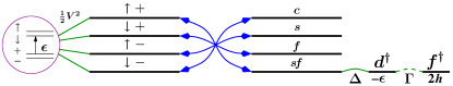
Figure 1: Schematic representation of the mapping procedure between the anisotropic two-channel Anderson model and the biresonant-level model. The external field enters as a site energy for the $f^{\dagger}$ fermion and has the effect of coupling its otherwise disconnected Majorana component.

Rewriting the $H_{\text{field}}$ term after the mapping, we find $H_{\text{field}}=H_{\text{field}}^{2}+H_{\text{field}}^{4}$ with

$$H_{\text{field}}^{2} =h\left(2n_{f}-1\right)-\lambda_{h}\left(n_{d}+n_{f}-\tfrac{1}{2}\right)~{}\text{,}$$ (49a)

$$H_{\text{field}}^{4} =2\lambda_{h}n_{f}n_{d}~{}\text{,}$$ (49b)

where we defined $\lambda_{h}=h_{f}-h_{s}$ and $2h=h_{f}+h_{s}$. Taking $\lambda_{h}=0$ we find that the model is still quadratic even for non-zero $h$. Nevertheless, we will see below that the presence of this term changes the fixed point; we will talk in this case of a double-Fermi biresonant-level model.

It is interesting to compare these two resonant-level models between them and with the models that correspond to the solvable points of the single- and two-channel Kondo models. In the latter cases, one obtains a single-Majorana resonant-level model and a single-Fermi resonant-level model, respectively. In contrast to the Kondo models, the Anderson case requires two fermionic degrees of freedom to parametrize the state of the impurity, which is now more complex, since it allows for fluctuating states of valence. For both the two-channel Kondo and Anderson models, in the absence of external fields, “half of a fermion” coming from the impurity decouples from the band and the models are naturally written in terms of the Majorana components of the impurity degrees of freedom. The Majorana component that exists completely decoupled from the rest of the system is responsible for the fractional residual impurity entropy that we will discuss below and constitutes a signature of the non-Fermi-liquid properties of the fixed point. In both cases, the addition of an external field has the effect of coupling the disconnected Majorana component and driving the system toward a Fermi-liquid type of fixed point, like the one of the single-channel Kondo model.

IV Stability of the Fixed Points

As mentioned above, taking $\lambda_{x}=0$ (for $x=c$, $s$, $f$, $s\!f$, $h$) defines a solvable manifold that contains a set of fixed points. The important question to be addressed is how generic and stable are those fixed points, how are they parametrized and whether RG-flow trajectories starting outside the manifold will flow to the same fixed points. The last consideration is particularly important, since it addresses the genericalness of the fixed points and the feasibility of perturbative calculations in $\lambda_{x}$.

IV.1 Inside the soluble manifold

In order to address these questions, we start by computing the different Green functions. For that, we first write down the local action for the impurity, in which the extended degrees of freedom from the band were integrated out exactly; this procedure is justified in order to study the interaction of the band with a local impurity that exists only at, say, $x_{\text{imp}}=0$. In Nambu notation, we write all the sums over positive Matsubara frequencies ($\omega_{n}$) only and use the following spinor basis:

$$\Psi(\omega_{n})\equiv\left(\begin{array}[c]{cccccc}\psi_{s\!f}\left(\omega_{n}\right)&\psi_{s\!f}^{\dagger}\left(-\omega_{n}\right)&d\left(\omega_{n}\right)&d^{\dagger}\left(-\omega_{n}\right)&f\left(\omega_{n}\right)&f^{\dagger}\left(-\omega_{n}\right)\end{array}\right)^{T}~{}\text{.}$$ (50)

The explicit form of the local action in the solvable manifold is

$$S=\frac{1}{\beta}\sum_{n\geq 0}\Psi^{\dagger}(\omega_{n})A(\omega_{n})\Psi(\omega_{n})~{}\text{,}$$ (51)

where $\beta=1/k_{\text{B}}T$ is the inverse temperature and

$$A(\omega_{n})=\left(\begin{array}[c]{cccccc}-2iv_{\text{F}}&0&\sqrt{2\Delta}&0&0&0\\ 0&-2iv_{\text{F}}&0&-\sqrt{2\Delta}&0&0\\ \sqrt{2\Delta}&0&-i\omega_{n}-\varepsilon&0&\sqrt{2\Gamma}&-\sqrt{2\Gamma}\\ 0&-\sqrt{2\Delta}&0&-i\omega_{n}+\varepsilon&\sqrt{2\Gamma}&-\sqrt{2\Gamma}\\ 0&0&\sqrt{2\Gamma}&\sqrt{2\Gamma}&-i\omega_{n}+2h&0\\ 0&0&-\sqrt{2\Gamma}&-\sqrt{2\Gamma}&0&-i\omega_{n}-2h\end{array}\right)~{}\text{.}$$ (52)

The two-point Green functions are defined as $\beta G(\omega_{n})\equiv\left\langle\Psi(\omega_{n})\Psi^{\dagger}(\omega_{n})\right\rangle$ with $G(\omega_{n})=A^{-1}(\omega_{n})$. Given the structure of the model, it is convenient to work in terms of Majorana fermions.Maldacena and Ludwig (1997) For that, we rotate each spinor according to

$$\Psi_{M}(\omega_{n})\equiv R\Psi(\omega_{n})=\left(\begin{array}[c]{cccccc}\psi_{s\!f}^{\prime\prime}\left(\omega_{n}\right)&\psi_{s\!f}^{\prime}\left(\omega_{n}\right)&d^{\prime\prime}\left(\omega_{n}\right)&d^{\prime}\left(\omega_{n}\right)&f^{\prime\prime}\left(\omega_{n}\right)&f^{\prime}\left(\omega_{n}\right)\end{array}\right)^{T}~{}\text{,}$$ (53)

where $R$ is a block diagonal matrix in which each block, given by

$$r=\frac{1}{\sqrt{2}}\begin{pmatrix}-i&i\\ 1&1\end{pmatrix}~{}\text{,}$$ (54)

rotates a given Nambu doublet. With this convention, the Majorana Green function matrix is $G_{M}(\omega_{n})=RG(\omega_{n})R^{\dagger}$ and its expression in imaginary time is

$$G_{M}(\tau-\tau^{\prime}) \equiv\left\langle\Psi_{M}(\tau)\Psi_{M}^{\dagger}(\tau^{\prime})\right\rangle$$

$$=\frac{1}{\beta}\sum_{n\geqslant 0}G_{M}(\omega_{n})e^{-i\omega_{n}\left(\tau-\tau^{\prime}\right)}$$

$$\qquad-G_{M}^{T}(\omega_{n})e^{i\omega_{n}\left(\tau-\tau^{\prime}\right)}~{}\text{.}$$ (55)

Let us now discuss the situation when $h=0$ (the case of $h\neq 0$ will be discussed in the Appendix). A direct calculation gives the following results for the long-$\tau$ behavior of the different diagonal Green functions:

$$\left\langle\psi_{s\!f}^{\prime\prime}(\tau)\psi_{s\!f}^{\prime\prime}(0)\right\rangle \sim\frac{1}{\tau}~{}\text{,} \left\langle\psi_{s\!f}^{\prime}(\tau)\psi_{s\!f}^{\prime}(0)\right\rangle \sim\frac{1}{\tau^{3}}~{}\text{,}$$ (56a)

$$\left\langle d^{\prime\prime}(\tau)d^{\prime\prime}(0)\right\rangle \sim\frac{1}{\tau}~{}\text{,} \left\langle d^{\prime}(\tau)d^{\prime}(0)\right\rangle \sim\frac{1}{\tau^{3}}~{}\text{,}$$ (56b)

$$\left\langle f^{\prime\prime}(\tau)f^{\prime\prime}(0)\right\rangle \sim\frac{1}{\tau}~{}\text{,} \left\langle f^{\prime}(\tau)f^{\prime}(0)\right\rangle \sim\operatorname*{sign}\tau~{}\text{.}$$ (56c)

Notice that different Majorana components of a given fermion exhibit different asymptotics; this fact and the $$1/\tau^{3} [\psi_{s\!f}^{\prime\prime}]=[d^{\prime\prime}]=[f^{\prime\prime}]=1/2 [\psi_{s\!f}^{\prime}]=[d^{\prime}]=3/2 [f^{\prime}]=0 \left\langle\psi_{s\!f}^{\prime\prime}(\tau)d^{\prime\prime}(0)\right\rangle\sim 1/\tau^{3}$$ behavior of certain Green functions were already stressed previously in the context of the two-channel Kondo model.Ye (1997, 1998) From these correlators, one could read the following naive scaling dimensions (see also Fig. 2): , , and . The long time behavior of all but one of the mixed correlation functions can be obtained using these scaling dimensions; the exception being .

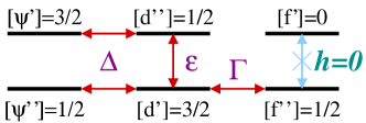
Figure 2: Connectivity graph, in terms of Majorana operators, for the biresonant-level model. The scaling dimensions of the fields are seen to alternate between $1/2$ and $3/2$, with the exception of $f^{\prime}$ that stays decoupled (for $h=0$) and has zero scaling dimension.

The scaling dimensions above are not compatible with a standard renormalization group scheme that proceeds by integrating energy shells while keeping certain coefficients of the quadratic action constant, cf. Ref. Shankar, 1994. Instead, we follow the ideas of Ref. Moustakas and Fisher, 1996 and introduce the Majorana Fermi velocities ($v_{\psi^{\prime}}$, $v_{\psi^{\prime\prime}}$) as well as constants multiplying the frequency in the Berry terms for the impurity ($g_{d^{\prime}}$, $g_{d^{\prime\prime}}$, $g_{f^{\prime}}$, $g_{f^{\prime\prime}}$) and let all of them vary. Specifically, we proceed along the standard stepsShankar (1994) but insisting that the fields should scale with the dimensions we determined from the Green functions, this yields the following RG-flow equations for the different couplings:

$$\frac{dg_{d^{\prime}}}{d\ell} =-3g_{d^{\prime}}~{}\text{,} \frac{dg_{d^{\prime\prime}}}{d\ell} =-g_{d^{\prime\prime}}~{}\text{,}$$ (57a)

$$\frac{dg_{f^{\prime}}}{d\ell} =0~{}\text{,} \frac{dg_{f^{\prime\prime}}}{d\ell} =-g_{f^{\prime\prime}}~{}\text{,}$$ (57b)

$$\frac{dv_{\psi^{\prime}}}{d\ell} =-2v_{\psi^{\prime}}~{}\text{,} \frac{dv_{\psi^{\prime\prime}}}{d\ell} =0~{}\text{,}$$ (57c)

$$\frac{d\Delta}{d\ell} =-\Delta~{}\text{,} \frac{d\varepsilon}{d\ell} =-\varepsilon~{}\text{,}$$ (57d)

$$\frac{d\Gamma}{d\ell} =-\Gamma~{}\text{,} \frac{dh}{d\ell} =\frac{1}{2}h~{}\text{.}$$ (57e)

We find that most couplings are RG-irrelevant but for $$v_{\psi^{\prime\prime}} g_{f^{\prime}} h=0 \varepsilon/\Delta$$ and that are RG-marginal. In here, we are considering , but we find that if a field were to be generated it would be RG-relevant. It is important to remark that the the quotient obeys

$$\frac{d}{d\ell}\left(\frac{\varepsilon}{\Delta}\right)=0$$ (58)

and is also marginal. This agrees with the results of Bethe ansatzBolech and Andrei (2002, 2005) and boundary conformal field theoryJohannesson et al. (2003) that find a line of non-Fermi-liquid fixed points that, in the microscopic theory, are parametrized by the $\varepsilon/\Delta$ ratio and interpolate between spin and flavor two-channel Kondo behaviors.

IV.2 Outside the soluble manifold

Collecting the terms in the refermionized Hamiltonian that takes us away from the soluble manifold, we have

$$H_{\lambda} =-\lambda_{c}\rho_{c}-\lambda_{s\!f}\rho_{s\!f}-\lambda_{s}\rho_{s}$$

$$+2\lambda_{c}\rho_{c}n_{d}+2\lambda_{s\!f}\rho_{s\!f}n_{d}+\lambda_{f}\rho_{f}n_{d}$$

$$+\lambda_{s}\rho_{s}n_{d}+2\lambda_{s}\rho_{s}n_{f}$$

$$-2\lambda_{f}\rho_{f}n_{d}n_{f}-2\lambda_{s}\rho_{s}n_{d}n_{f}$$

$$-\lambda_{h}\left(n_{d}+n_{f}-\tfrac{1}{2}\right)+2\lambda_{h}n_{f}n_{d}~{}\text{.}$$ (59)

In order to determine the stability of the $h=0$ fixed points, we proceed to study the RG-relevance of the different terms in $H_{\lambda}$. The first three terms are just chemical potential terms for the conduction electrons. The charge and spin ones pertain only to bands that are decoupled from the impurity and are marginal operators, since the dimension of the respective fields is $1/2$, as dictated by their Berry phases. On the other hand, the spin-flavor one is irrelevant as can be seen by simple power counting.

For the operators in the second, third and fourth lines, we get the following dimensions by summing the dimensions of their constituents $[\rho_{c}n_{d}]=[\rho_{f}n_{d}]=[\rho_{s}n_{d}]=3$, $[\rho_{s\!f}n_{d}]=4$, $[\rho_{s}n_{f}]=3/2$ and $[\rho_{f}n_{d}n_{f}]=[\rho_{s}n_{d}n_{f}]=7/2$. Hence, all of them are RG-irrelevant. None of these terms can generate a local field term for the impurity. In particular, $\psi_{c}$, $\psi_{s}$ and $\psi_{f}$ are decoupled (and the average of the normal-ordered densities $\rho_{c}$, $\rho_{s}$ and $\rho_{f}$ is zero). Eventually, the operator $\rho_{s\!f}n_{d}$ may give a correction to $\varepsilon$, thus taking the system along the line of fixed points.

An interesting situation appears when one starts from the fixed point in the absence of a magnetic field ($h_{s}=0$) and considers the effect of a small $\lambda_{h}\neq 0$ (this is realized when one starts with $\lambda_{h}=2h$, or in other words, with $h_{f}\neq 0$). Then one must consider carefully the effect of the last term in $H_{\lambda}$, with dimension $[n_{f}n_{d}]=5/2$ and therefore, in principle, RG-irrelevant. This term is actually classified as dangerously irrelevant, as it generates a potential field for $f$ (i.e., an RG-relevant $h$ term). It thus couples the remaining Majorana component, $f^{\prime}$, and changes the fixed point.

Indeed, when adding a magnetic field the fixed point changes (see Appendix). The chemical potentials for $\psi_{sf}$ and $d$ become marginal, and the operators with four and six fermions are now all irrelevant. The parameters $\varepsilon/\Delta$ and $h/\Gamma$ parametrize the new set of Fermi-liquid fixed points.

V Thermodynamics with Finite Field

In order to extract the impurity thermodynamics when the model parameters are on the solvable manifold, we can resort to an exact calculation of the free energy. The impurity free energy can be straightforwardly calculated by means of Pauli’s trick of integration over the coupling constants (an alternative way is to first derive an effective action for the impurityGan (1995)), namely,

$$\Omega-\Omega_{0}=\int_{0}^{1}\frac{d\xi}{\xi}~{}\left\langle\xi\left(H_{\text{biRes}}-H_{0}^{s\!f}\right)\right\rangle_{\xi}~{}\text{.}$$ (60)

The $\xi$ subindex indicates that the mean values should be computed using an action in which all couplings involving the impurity were multiplied by the dimensionless parameter $\xi$, and $\Omega_{0}$ is the impurity free energy when $\xi=0$. After computing the mean values using $G_{\xi}\left(\omega_{n}\right)$, one arrives at the expression

$$\Omega-\Omega_{0}=-\int_{0}^{1}d\xi~{}\frac{1}{\beta}\sum_{n\geq 0}\frac{\partial_{\xi}D\left(\omega_{n},\xi\right)}{D\left(\omega_{n},\xi\right)}~{}\text{,}$$ (61)

where

$$D(\omega_{n},\xi) \equiv-\frac{1}{4}\det A_{\xi}\left(\omega_{n}\right)=4h^{2}\Delta^{2}\xi^{6}$$

$$+\left[\Delta\omega_{n}\left(8\Gamma+\Delta\omega_{n}\right)+4h^{2}\left(\varepsilon^{2}+2\Delta\omega_{n}\right)\right]\xi^{4}$$

$$+\omega_{n}^{2}\left(4h^{2}+8\Gamma+\varepsilon^{2}+2\Delta\omega_{n}\right)\xi^{2}+\omega_{n}^{4}~{}\text{.}$$ (62)

As a function of $\omega_{n}$, this is a fourth order polynomial with roots that are parametric functions of $\xi$: $\omega_{k}\left(\xi\right)$, $k=0,\ldots,3$. Using the factorized form of the polynomial in terms of its roots and introducing a suitable regularization, we arrive at the following expression:

$$\Omega-\Omega_{0} =\int_{0}^{1}d\xi\frac{1}{\beta}\sum_{n\geq 0}\sum_{k}\frac{\partial_{\xi}\omega_{k}(\xi)}{\omega_{n}-\omega_{k}(\xi)}$$

$$=\int_{0}^{1}d\xi\frac{1}{\beta}\sum_{n\geq 0}\sum_{k}\partial_{\xi}\omega_{k}(\xi)\int_{-\Lambda}^{\omega_{k}(\xi)}d\mu\frac{1}{\left[\omega_{n}-\mu\right]^{2}}~{}\text{.}$$ (63)

We verify that $\omega_{k}(0)=0$ and call $\omega_{k}\equiv\omega_{k}\left(1\right)$. Exchanging the sum in $n$ and the integral in $\mu$, we arrive at the final expression:

$$\Omega-\Omega_{0}=\sum_{k}\frac{1}{2\pi}\left[\psi\left(\frac{1}{2}+\frac{\Lambda\beta}{2\pi}\right)\omega_{k}\right.\\ +\left.\frac{2\pi}{\beta}\ln\Gamma\left(\frac{1}{2}-\frac{\omega_{k}\beta}{2\pi}\right)-\frac{2\pi}{\beta}\ln\Gamma\left(\frac{1}{2}\right)\right]~{}\text{,}$$ (64)

where $\psi\left(z\right)\equiv\partial_{z}\ln\Gamma\left(z\right)$ is the digamma function. Note that the free energy needs the $\Lambda$ regulator, but in all the derived thermodynamic quantities we will be able to take the the limit $\Lambda\rightarrow+\infty$ and obtain finite results.

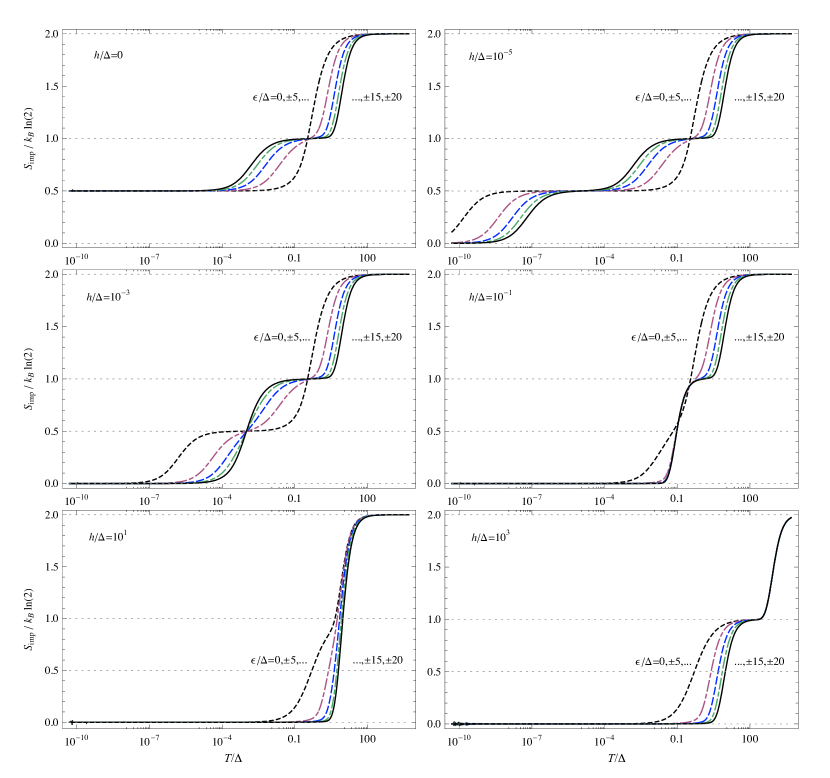
Figure 3: Impurity contribution to the entropy as a function of temperature for different values of the symmetric external field $h$. Temperature and field are both measured in units of $\Delta$. Different curves correspond to different values of $\varepsilon/\Delta$ and $\Gamma=\Delta/2\pi$. The top left panel corresponds to zero field and the other ones to finite values of the field that increase hundredfold between panels, from $h=10^{-5}\Delta$ until $h=10^{3}\Delta$.

In particular, the impurity entropy is given by $S-S_{0}=\sum_{k}s\left(z_{k}\right)$, with $z_{k}=-\beta\omega_{k}/2\pi$ and

$$s\left(z\right)=z\left[\psi\left(\frac{1}{2}+z\right)-1\right]-\ln\Gamma\left(\frac{1}{2}+z\right)+\frac{1}{2}\ln\pi~{}\text{.}$$ (65)

Remarkably, the function $s\left(z\right)$ is the same that is found for the entropy of the two-channel Kondo model on the Emery-Kivelson line. Fabrizio et al. (1995) This is not completely unexpected, since Kondo is the low-energy effective theory for most part of the parameter regime of the two-channel Anderson model. In Fig. 3, we show the impurity contribution to the entropy as a function of temperature for different values of the local field $h$.

Let us first discuss the $h=0$ case shown on the top left panel of the figure. In this case, one of the roots is zero ($\omega_{3}=0$) and there is a residual entropy of $S_{\text{imp}}=k_{\text{B}}\ln\sqrt{2}$ that signals a non-Fermi-liquid set of fixed points. The finite temperature physics is governed by the other three roots.Bolech and Iucci (2006a) We find that, within the range of parameters of physical relevance, one of the roots ($\omega_{0}$) is real while the other two ($\omega_{1,2}$) are complex conjugate of each other. This makes it natural to identify the roots with the Kondo and Schottky energy scales in the following way:

$$k_{\text{B}}T_{\text{K}} =-\omega_{0}/2\pi~{}\text{,}$$ (66)

$$k_{\text{B}}T_{\text{S}} =\left|\omega_{1}\right|/2\pi~{}\text{.}$$ (67)

The Kondo scale corresponds to a jump in the entropy of hight $k_{\text{B}}\ln\sqrt{2}$, while the Schottky scale is associated with a jump that is twice as large. For small $\left|\varepsilon\right|$, the two quenching steps coincide; whereas as $\left|\varepsilon\right|/\Delta$ grows, the Kondo temperature decreases while the Schottky temperature increases. Evidently, over the soluble manifold, the dependence of all scales on the microscopic parameters is algebraic. This contrasts with the isotropic case, for which the Kondo scale has exponential dependence on $\left|\varepsilon\right|/\Delta$.Bolech and Andrei (2005) This behavior is seen also in the single- and two-channel Kondo models, for which it is found that the exponential dependence of the Kondo scale is a property of the isotropic models only and the functional dependence crosses over to algebraic in the Toulouse and Emery-Kivelson limits, respectively.Tsvelik and Wiegmann (1983); Zaránd et al. (2002) Another characteristic of the solvable limit is that the $\ln T$ dependencies in the impurity susceptibilities or in the specific heat coefficient are changed into power laws. It is known that the logarithms can be recovered using perturbation theory in $\lambda_{\nu}$ (cf. Refs. Emery and Kivelson, 1992; Clarke et al., 1993; Sengupta and Georges, 1994), as it reintroduces the leading RG-irrelevant operators that are absent from the soluble manifold. For the leading contribution, the three operators with scaling dimension $3$ (i.e., $\rho_{c}n_{d}$, $\rho_{s}n_{d}$, and $\rho_{f}n_{d}$) can be included using second-order perturbation theory in the couplings. All three of them mix one of the decoupled bands and the impurity in a way that is the direct generalization of what happens in the case of the two-channel Kondo model.Sengupta and Georges (1994) Such a procedure should recover, for instance, not only the results for the specific heat and susceptibilities but also the Wilson ratio that was discussed already in Ref. Johannesson et al., 2003.

When $h\neq 0$, $\omega_{3}$ becomes non-zero as well and grows with $h$. This introduces a third quenching step (as it can be seen, for instance, in the top right panel of the figure) in which the entropy goes from $k_{\text{B}}\ln\sqrt{2}$ to zero, signaling the system flowing away from the non-Fermi-liquid fixed point. This is in accordance with the result of the previous section, in which we found $h$ to be a relevant perturbation. This process defines a third energy scale,

$$k_{\text{B}}T_{h}=-\omega_{3}/2\pi~{}\text{,}$$ (68)

that grows with $h$ until reaching the same value as $T_{\text{K}}$, –which happens at different values of the field for different values of $\left|\varepsilon\right|$ (taking place first for larger values, see the middle left panel in Fig. 3). As these two energy scales merge, the respective roots become a complex-conjugate pair, a single quenching step of the same height as the Schottky one emerges and the transition width (i.e., the width of the corresponding anomaly in the specific heat) narrows. As $h$ increases further, the three scales first become degenerate and then cross each other. In the bottom right panel, the two scales have already crossed, the higher temperature step is given by $T_{\text{K}}=T_{h}$ and is insensitive to the value of $\left|\varepsilon\right|/\Delta$, while the lower one continues to correspond to the Schottky transition and shows the same type of dependence in $\left|\varepsilon\right|/\Delta$ as for lower fields. These results share many properties with those for the isotropic case, but they are specific to the case of a symmetric filed ($\lambda_{h}=0$) and exhibit important differences with the case when only $h_{s}$ or $h_{f}$ is applied to the system (cf. Fig. 7 in Ref. Bolech and Andrei, 2005).

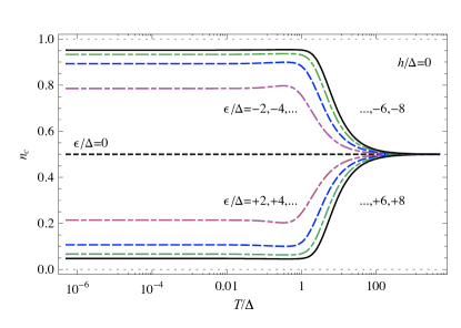
Figure 4: Impurity charge valence as a function of temperature. The curves are displayed for $h=0$, the only effect of finite fields is to wash out the overshoot that happens for small values of $\varepsilon/\Delta$ and to shift (away from $1/2$) the zero-temperature values of $n_{c}$ (see text).

Other thermodynamic quantities of interest are the impurity charge valence $n_{c}=\partial\Omega/\partial\varepsilon$ and the magnetization $m_{\text{imp}}=-\partial\Omega/\partial h$. They are explicitly given by the expressions:

$$n_{c}-n_{c,0} =\frac{1}{\beta}\sum_{k}\psi\left(\frac{1}{2}+z_{k}\right)\partial_{\varepsilon}z_{k}~{}\text{,}$$ (69a)

$$m_{\text{imp}}-m_{\text{imp},0} =-\frac{1}{\beta}\sum_{k}\psi\left(\frac{1}{2}+z_{k}\right)\partial_{h}z_{k}~{}\text{,}$$ (69b)

where the derivatives of the roots can be expressed in closed form using the identity

$$\partial_{\varepsilon,h}\omega_{k}=-\frac{\left.\partial_{\varepsilon,h}D(\omega,1)\right|_{\omega=\omega_{k}}}{\prod_{j\neq k}\left(\omega_{k}-\omega_{j}\right)}~{}\text{.}$$ (70)

Plots of these two quantities are displayed in Figs. 4 and 5, respectively.

The variability of the impurity valence is an aspect inherent to Anderson-type models and of relevance, for instance, in the context of quantum dots and other mesoscopic systems that might allow direct measurements of the valence states via changes in capacitance.Bolech and Shah (2005) The valence starts as $n_{c,0}=1/2$ at high temperature ($T\gg T_{\text{S}}$) independently of the values of $\varepsilon$ and $h$, and evolves as the temperature is lowered to attain a certain zero-temperature value $n_{c}^{0}\equiv n_{c}\left(\varepsilon,h\right)_{T=0}$ that characterizes the particular fixed point that the system reaches. The quenching of the valence fluctuations coincides with the first quenching of the entropy and takes place at the characteristic scale $T_{\text{S}}$. Subtle aspects of the small $\left|\varepsilon\right|$ curves, such as the “overshoot” of the curves at intermediate temperatures, $T\lesssim T_{\text{S}}$, are generic and are also present in the exact solution of the isotropic model.Bolech and Andrei (2005); Bolech and Iucci (2006a, b) This feature exists for $h$ zero or small and disappears as $h$ becomes of the order of $\Delta$. Comparisons with the isotropic model show that, despite the differences in the infrared physics, the isotropic and the anisotropic models share the same generic ultraviolet physics.Bolech and Iucci (2006a) This is to be expected, since the physics at higher energies tends to be dominated by local fluctuations.

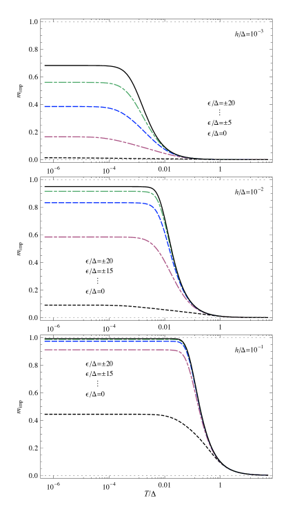
Figure 5: Impurity magnetization versus temperature. From top to bottom, the three panels show three different values of $h/\Delta=10^{-3},10^{-2},10^{-1}$. Curves for different values of $\varepsilon/\Delta$ are shown and the values are indicated in the figure.

The curves of finite-field impurity magnetization as a function of temperature are in some ways similar to those of the charge valence. At high temperatures, the magnetization is zero, and it acquires a field-dependent finite value as the temperature becomes $T\lesssim T_{h}$ (the magnetization does not reach the maximum value of $1$ due to the hybridization of the impurity with the conduction band). In this case, curves for positive and negative values of $\varepsilon$ are degenerate. The quantities $m_{\text{imp}}^{0}\equiv m_{\text{imp}}\left(\varepsilon,h\right)_{T=0}$ and $n_{c}^{0}$ label the set of finite-field fixed points of the model. As we mentioned above, these fixed points are of the local Fermi-liquid type.

VI Conclusion

We have shown how the addition of exchange terms that provide anisotropy that breaks the $SU\left(2\right)$ symmetry of the two-channel Anderson model in the spin and flavor sectors, by singling out an easy access for each of them, allows to identify a manifold in coupling constant space over which the model becomes quadratic and thus exactly solvable. The solvable theory is obtained in the form of a mapping to an anusual type of resonant-level model that includes two resonant levels and we thus call it a biresonant-level model. Similar mappings exist for the Kondo model in the case of one and two channels (and are known to be impossible for larger number of channelsTsvelik (1995)). But a simple mapping of this type is new for a model like the two-channel Anderson model that incorporates the physics of valence fluctuations. Equivalent mappings for the single-channel Anderson model are elusive (cf. Ref. Kotliar and Si, 1996), which indicates that the case of the two-channel model constitutes a singular example. Since the mapping captures, in particular, the mixed valence regime of the model, –in which electrons fluctuate from the impurity to the band and vice versa–, it is of utmost importance to verify that such physics is rigorously captured by including the Klein factors and showing how they take part in the transformations that are required for the mapping. A careful study of the Klein factors opens the door for future calculations of correlation functions using the solvable points as starting ground. The representativity of calculations that start from the biresonant-level model requires that such model flows into generic fixed points representative of the physics of the original model. We performed an analysis of the stability of deviations from the locus of solvable points in parameter space and established that perturbation theory on such deviations is valid. The advantage of starting from the mapped model is evident: closed analytical expressions can be derived for the full temperature crossovers of the different quantities of interest; this sets the approach apart from other non-perturbative techniques applied previously to the two-channel Anderson model.

To illustrate the versatility, power and simplicity of the use of the biresonant-level model to do calculations, we presented several results of thermodynamic quantities that involve the impurity. Namely, we gave results for the impurity entropy, valence and magnetization as functions of temperature for different values of $\varepsilon$ and $h$. These quantities illustrate the existence of several energy scales in the model that signal the transitions between different regimes. It is remarkable that all the crossovers can be calculated explicitly in closed analytic expressions, something not possible with other types of calculations.

For the followup, it would be interesting to exploit the precise mapping (that includes all the details such as Klein factors, decoupled bands, etc.) to compute dynamic correlation functions involving the impurity. Another interesting direction would be the study of the finite-size crossover spectrum of the model, which would allow to establish instructive connections with different renormalization group schemes. Finally, we are in a position to, for instance, consider the behavior of more than one impurity (cf. Ref. Ferrero et al., 2007) and, in particular, the case of one-dimensional two-channel Anderson lattices (cf. Ref. Schauerte et al., 2005). The latter would be interesting in order to determine if lattice effects are able to reverse the sign of the prefactor in the leading $\sqrt{T}$ term in the resistivity,Johannesson et al. (2005) which would be required in order to match the experimental results for thoriated UBe₁₃.Aliev et al. (1995); Dickey et al. (1997)

Appendix: Study of the finite-field fixed points

The long-$\tau$ asymptotics change dramatically when a non-zero external field is present ($h\neq 0$). The $f^{\prime}$ Majorana component of $f$ is now coupled to the rest of the system and we must recompute all the Green functions. For the diagonal ones, we find

$$\left\langle\psi_{s\!f}^{\prime\prime}(\tau)\psi_{s\!f}^{\prime\prime}(0)\right\rangle \sim\frac{1}{\tau}~{}\text{,} \left\langle\psi_{s\!f}^{\prime}(\tau)\psi_{s\!f}^{\prime}(0)\right\rangle \sim\frac{1}{\tau}~{}\text{,}$$ (71a)

$$\left\langle d^{\prime\prime}(\tau)d^{\prime\prime}(0)\right\rangle \sim\frac{1}{\tau}~{}\text{,} \left\langle d^{\prime}(\tau)d^{\prime}(0)\right\rangle \sim\frac{1}{\tau}~{}\text{,}$$ (71b)

$$\left\langle f^{\prime\prime}(\tau)f^{\prime\prime}(0)\right\rangle \sim\frac{1}{\tau^{3}}~{}\text{,} \left\langle f^{\prime}(\tau)f^{\prime}(0)\right\rangle \sim\frac{1}{\tau}~{}\text{,}$$ (71c)

from where we read the new naive scaling dimensions: $$[\psi_{s\!f}^{\prime\prime}]=[\psi_{s\!f}^{\prime}]=[d^{\prime\prime}]=[d^{\prime}]=[f^{\prime}]=1/2 [f^{\prime\prime}]=3/2 \tau$$ and . For the nondiagonal Green functions, the following ones have long- behaviors that do not match the expectations from the naive scalings:

$$\left\langle\psi_{s\!f}^{\prime}(\tau)\psi_{s\!f}^{\prime\prime}(0)\right\rangle \sim\dfrac{1}{\tau^{2}}~{}\text{,} \left\langle\psi_{s\!f}^{\prime}(\tau)d^{\prime\prime}(0)\right\rangle \sim\dfrac{1}{\tau^{2}}~{}\text{,}$$ (72a)

$$\left\langle\psi_{s\!f}^{\prime\prime}(\tau)d^{\prime}(0)\right\rangle \sim\dfrac{1}{\tau^{2}}~{}\text{,} \left\langle\psi_{s\!f}^{\prime\prime}(\tau)f^{\prime\prime}(0)\right\rangle \sim\dfrac{1}{\tau^{3}}~{}\text{,}$$ (72b)

$$\left\langle\psi_{s\!f}^{\prime\prime}(\tau)f^{\prime}(0)\right\rangle \sim\dfrac{1}{\tau^{2}}~{}\text{,} \left\langle d^{\prime\prime}(\tau)d^{\prime}(0)\right\rangle \sim\dfrac{1}{\tau^{2}}~{}\text{,}$$ (72c)

$$\left\langle d^{\prime\prime}(\tau)f^{\prime\prime}(0)\right\rangle \sim\dfrac{1}{\tau^{3}}~{}\text{,} \left\langle d^{\prime\prime}(\tau)f^{\prime}(0)\right\rangle \sim\dfrac{1}{\tau^{2}}~{}\text{.}$$ (72d)

All of them decay faster than what the naive use of the scaling dimensions of the fields would indicate. Thus, in order to obtain the RG flow of the nondiagonal couplings, one should, all the same, employ the naive dimensions. The resulting flow equations are as follows:

$$\frac{dg_{d^{\prime}}}{d\ell} =-g_{d^{\prime}}~{}\text{,} \frac{dg_{d^{\prime\prime}}}{d\ell} =-g_{d^{\prime\prime}}~{}\text{,}$$ (73a)

$$\frac{dg_{f^{\prime}}}{d\ell} =-g_{f^{\prime}}~{}\text{,} \frac{dg_{f^{\prime\prime}}}{d\ell} =-3g_{f^{\prime\prime}}~{}\text{,}$$ (73b)

$$\frac{dv_{\psi^{\prime}}}{d\ell} =0~{}\text{,} \frac{dv_{\psi^{\prime\prime}}}{d\ell} =0~{}\text{,}$$ (73c)

$$\frac{d\Delta}{d\ell} =0~{}\text{,} \frac{d\varepsilon}{d\ell} =0~{}\text{,}$$ (73d)

$$\frac{d\Gamma}{d\ell} =-\Gamma~{}\text{,} \frac{dh}{d\ell} =-h~{}\text{.}$$ (73e)

Now $$h h/\Gamma$$ became RG-irrelevant. However, the ratio is exactly marginal and parametrizes the new finite-field Fermi-liquid fixed points.

References

- Cox (1987) D. L. Cox, Phys. Rev. Lett. 59, 1240 (1987), Erratum: ibid. 61, 1527 (1988).
- Nozières and Blandin (1980) P. Nozières and A. Blandin, J. Phys. (Paris) 41, 193 (1980).
- Kawae et al. (2006) T. Kawae, K. Kinoshita, Y. Nakaie, N. Tateiwa, K. Takeda, H. S. Suzuki, and T. Kitai, Phys. Rev. Lett. 96, 027210 (2006).
- Cox and Zawadowski (1998) D. L. A. Cox and A. Zawadowski, Adv. Phys. 47, 599 (1998).
- Hotta (2005) T. Hotta, Phys. Rev. Lett. 94, 067003 (2005).
- Hotta (2006) T. Hotta, Phys. Rev. Lett. 96, 197201 (2006).
- Ramirez et al. (1994) A. P. Ramirez, P. Chandra, P. Coleman, Z. Fisk, J. L. Smith, and H. R. Ott, Phys. Rev. Lett. 73, 3018 (1994).
- Aliev et al. (1995) F. G. Aliev, H. E. Mfarrej, S. Vieira, R. Villar, and J. L. Martinez, Europhys. Lett. 32, 765 (1995).
- Harrison et al. (2001) N. Harrison, L. Balicas, A. A. Teklu, R. G. Goodrich, J. S. Brooks, J. C. Cooley, and J. L. Smith, Phys. Rev. B 63, 081101(R) (2001).
- Schiller et al. (1998) A. Schiller, F. B. Anders, and D. L. Cox, Phys. Rev. Lett. 81, 3235 (1998).
- Koga and Cox (1999) M. Koga and D. L. Cox, Phys. Rev. Lett. 82, 2575 (1999).
- Bolech and Andrei (2002) C. J. Bolech and N. Andrei, Phys. Rev. Lett. 88, 237206 (2002).
- Onimaru et al. (2005) T. Onimaru, T. Sakakibara, N. Aso, H. Yoshizawa, H. S. Suzuki, and T. Takeuchi, Phys. Rev. Lett. 94, 197201 (2005).
- Bauer et al. (2002) E. D. Bauer, N. A. Frederick, P.-C. Ho, V. S. Zapf, and M. B. Maple, Phys. Rev. B 65, 100506(R) (2002).
- Bauer et al. (2006) E. D. Bauer, P.-C. Ho, M. B. Maple, T. Schauerte, D. L. Cox, and F. B. Anders, Phys. Rev. B 73, 094511 (2006).
- Maple (2005) M. B. Maple, J. Phys. Soc. Jpn. 74, 222 (2005).
- Berman et al. (1999) D. Berman, N. B. Zhitenev, R. C. Ashoori, and M. Shayegan, Phys. Rev. Lett. 82, 161 (1999).
- Oreg and Goldhaber-Gordon (2003) Y. Oreg and D. Goldhaber-Gordon, Phys. Rev. Lett. 90, 136602 (2003).
- Shah and Millis (2003) N. Shah and A. J. Millis, Phys. Rev. Lett. 91, 147204 (2003).
- Kakashvili and Johannesson (2007) P. Kakashvili and H. Johannesson, Europhys. Lett. 79, 47004 (2007).
- Potok et al. (2007) R. M. Potok, I. G. Rau, H. Shtrikman, Y. Oreg, and D. Goldhaber-Gordon, Nature (London) 446, 167 (2007).
- Bolech and Shah (2005) C. J. Bolech and N. Shah, Phys. Rev. Lett. 95, 036801 (2005).
- Kondo (1964) J. Kondo, Prog. Theor. Phys. 32, 37 (1964).
- Wilson (1975) K. G. Wilson, Rev. Mod. Phys. 47, 773 (1975).
- Andrei (1980) N. Andrei, Phys. Rev. Lett. 45, 379 (1980).
- Wiegmann (1980) P. B. Wiegmann, Phys. Lett. A 80, 163 (1980).
- Toulouse (1969) G. Toulouse, C. R. Acad. Sci. 268, 1200 (1969).
- Schlottmann (1978) P. Schlottmann, J. Phys. (Paris) 39, 1486 (1978).
- Vigman and Finkel’shteǐn (1978) P. B. Vigman and A. M. Finkel’shteǐn, Sov. Phys. JETP 48, 102 (1978).
- Hewson (1993) A. C. Hewson, The Kondo Problem to Heavy Fermions (Cambridge University Press, Cambridge, England, 1993).
- Kotliar and Si (1996) G. Kotliar and Q. Si, Phys. Rev. B 53, 12373 (1996).
- Bolech and Iucci (2006a) C. J. Bolech and A. Iucci, Phys. Rev. Lett. 96, 056402 (2006a).
- Andrei et al. (1983) N. Andrei, K. Furuya, and J. H. Lowenstein, Rev. Mod. Phys. 55, 331 (1983).
- Affleck (1995) I. Affleck, Acta Phys. Pol. B 26, 1869 (1995), lecture given at the XXXVth Cracow School of Theoretical Physics, Zakopane, Poland, June 4-14 1995.
- Giamarchi (2004) T. Giamarchi, Quantum Physics in One Dimension (Clarendon Press, Oxford, 2004).
- Emery and Kivelson (1992) V. J. Emery and S. Kivelson, Phys. Rev. B 46, 10812 (1992).
- Fabrizio et al. (1995) M. Fabrizio, A. O. Gogolin, and P. Nozières, Phys. Rev. B 51, 16088 (1995).
- Schofield (1997) A. J. Schofield, Phys. Rev. B 55, 5627 (1997).
- Ye (1997) J. Ye, Phys. Rev. B 56, R489 (1997).
- von Delft et al. (1998) J. von Delft, G. Zaránd, and M. Fabrizio, Phys. Rev. Lett. 81, 196 (1998).
- Johannesson et al. (2003) H. Johannesson, N. Andrei, and C. J. Bolech, Phys. Rev. B 68, 075112 (2003).
- Johannesson et al. (2005) H. Johannesson, C. J. Bolech, and N. Andrei, Phys. Rev. B 71, 195107 (2005).
- Anders (2005) F. B. Anders, Phys. Rev. B 71, 121101(R) (2005).
- Bolech and Andrei (2005) C. J. Bolech and N. Andrei, Phys. Rev. B 71, 205104 (2005).
- Haldane (1981) F. D. M. Haldane, J. Phys. C 14, 2585 (1981).
- von Delft and Schoeller (1998) J. von Delft and H. Schoeller, Annalen der Phys. 7, 225 (1998).
- Gogolin et al. (1998) A. O. Gogolin, A. A. Nersesyan, and A. M. Tsvelik, Bosonization and Strongly Correlated Systems (Cambridge University Press, Cambridge, England, 1998).
- Zaránd and von Delft (2000) G. Zaránd and J. von Delft, Phys. Rev. B 61, 6918 (2000).
- Clarke et al. (1993) D. G. Clarke, T. Giamarchi, and B. I. Shraiman, Phys. Rev. B 48, 7070 (1993).
- Sengupta and Georges (1994) A. M. Sengupta and A. Georges, Phys. Rev. B 49, R10020 (1994).
- Maldacena and Ludwig (1997) J. M. Maldacena and A. W. W. Ludwig, Nucl. Phys. B 506, 565 (1997).
- Ye (1998) J. Ye, Nucl. Phys. B 512, 543 (1998).
- Shankar (1994) R. Shankar, Rev. Mod. Phys. 66, 129 (1994).
- Moustakas and Fisher (1996) A. L. Moustakas and D. S. Fisher, Phys. Rev. B 53, 4300 (1996).
- Gan (1995) J. Gan, Phys. Rev. B 51, 8287 (1995).
- Tsvelik and Wiegmann (1983) A. M. Tsvelik and P. B. Wiegmann, Adv. Phys. 32, 453 (1983).
- Zaránd et al. (2002) G. Zaránd, T. Costi, A. Jerez, and N. Andrei, Phys. Rev. B 65, 134416 (2002).
- Bolech and Iucci (2006b) C. J. Bolech and A. Iucci, Physica B 378-80, 171 (2006b).
- Tsvelik (1995) A. M. Tsvelik, Phys. Rev. B 52, 4366 (1995).
- Ferrero et al. (2007) M. Ferrero, L. De Leo, P. Lecheminant, and M. Fabrizio, J. Phys.: Condens. Matter 19, 433201 (2007).
- Schauerte et al. (2005) T. Schauerte, D. L. Cox, R. M. Noack, P. G. J. van Dongen, and C. D. Batista, Phys. Rev. Lett. 94, 147201 (2005).
- Dickey et al. (1997) R. P. Dickey, M. C. de Andrade, J. Herrmann, M. B. Maple, F. G. Aliev, and R. Villar, Phys. Rev. B 56, 11169 (1997).