Inelastic effects
in molecular junction transport:
Scattering and self-consistent calculations
for the Seebeck coefficient

Abstract

The influence of molecular vibration on the Seebeck coefficient is studied within a simple model. Results of a scattering theory approach are compared to those of a full self-consistent nonequilibrium Green’s function scheme. We show, for a reasonable choice of parameters, that inelastic effects have non-negligible influence on the resulting Seebeck coefficient for the junction. We note that the scattering theory approach may fail both quantitatively and qualitatively. Results of calculation with reasonable parameters are in good agreement with recent measurements [P. Reddy et al., Science 315, 1568 (2007)]

1 Introduction

Development of experimental techniques for constructing and exploring molecular devices has inspired extensive theoretical study of charge transport in molecules, with potential application in molecular electronics.[1, 2, 3, 4] One important issue related to stability of potential molecular devices involves heating and heat transport in molecular junctions. This topic has attracted attention both experimentally[5, 6, 7, 8, 9, 10] and theoretically.[11, 12, 13, 14, 15, 16, 17, 18, 19, 20, 22] Another closely related issue involves thermoelectric properties of such devices. While thermo-electricity in bulk is well studied, corresponding measurements in molecular junctions were reported only recently.[23, 24]

Electron-vibration interactions in the junction (leading to inelastic effects in charge transport[21]) may cause junction heating and affect its heat transport properties.[22] Theoretical considerations of thermoelectric properties so far either completely disregarded such effects (in treatments based on the Landauer theory[24, 25, 26]) or included it within a scattering theory framework.[27, 28] The latter treats the effect of vibrations as an inelastic electron scattering process, and changes in the non-equilibrium distributions of electrons and vibrations are not described in a self-consistent manner. It has been shown that such changes may have qualitative effects on the transport.[30, 29] Note also that scattering theory approaches may lead to erroneous predictions due to neglecting effects of contacts’ Fermi seas on the junction electronic structure.[31]

This paper is motivated by recent measurements of the Seebeck coefficient in molecular junctions.[24] Considerations based on Landauer formula were employed there to interpret experimental data. Our goals here are: 1. to show the importance of vibrations for the Seebeck coefficient and 2. to include vibrations in a fully self-consistent way within the nonequilibrium Green’s function approach for calculating the Seebeck coefficient. The structure of the paper is the following. Section 2 introduces the model, discusses methods used in calculations, and presents a simple (approximate) analytical derivation to illustrate change in the Seebeck coefficient expression (as compared to Landauer-based expression) when vibrations are taken into account. Section 4 presents numerical results obtained in a fully self-consistent way. Section 5 concludes.

2 Model

We consider a simple resonant-level model with the electronic level $|0>$ coupled to two electrodes left ($L$) and right ($R$) (each a free electron reservoir at its own equilibrium). The electron on the resonant level (electronic energy $\varepsilon_{0}$) is linearly coupled to a single vibrational mode (referred below as primary phonon) with frequency $\omega_{0}$. The latter is coupled to a phonon bath represented as a set of independent harmonic oscillators (secondary phonons). The system Hamiltonian is (here and below we use $\hbar=1$ and $e=1$)

$$\hat{H}=\varepsilon_{0}\hat{c}^{\dagger}\hat{c}+\sum_{k\in\{L,R\}}\varepsilon_{k}\hat{c}_{k}^{\dagger}\hat{c}_{k}+\sum_{k\in\{L,R\}}\left(V_{k}\hat{c}_{k}^{\dagger}\hat{c}+\mbox{h.c.}\right)$$

$$+\omega_{0}\hat{a}^{\dagger}\hat{a}+\sum_{\beta}\omega_{\beta}\hat{b}^{\dagger}_{\beta}\hat{b}_{\beta}+M_{a}\hat{Q}_{a}\hat{c}^{\dagger}\hat{c}+\sum_{\beta}U_{\beta}\hat{Q}_{a}\hat{Q}_{\beta}$$ (1)

where $\hat{c}^{\dagger}$ ($\hat{c}$) are creation (destruction) operators for electrons on the bridge level, $\hat{c}_{k}^{\dagger}$ ($\hat{c}_{k}$) are corresponding operators for electronic states in the contacts, $\hat{a}^{\dagger}$ ($\hat{a}$) are creation (destruction) operators for the primary phonon, and $\hat{b}_{\beta}^{\dagger}$ ($\hat{b}_{\beta}$) are the corresponding operators for phonon states in the thermal (phonon) bath. $\hat{Q}_{a}$ and $\hat{Q}_{\beta}$ are phonon displacement operators

$$\hat{Q}_{a}=\hat{a}+\hat{a}^{\dagger}\qquad\hat{Q}_{\beta}=\hat{b}_{\beta}+\hat{b}_{\beta}^{\dagger}$$ (2)

The energy parameters $M_{a}$ and $U_{\beta}$ correspond to the vibronic and the vibrational coupling respectively. Eq.(2) is often used as a generic model for describing effects of vibrational motion on electronic conduction in molecular junctions.[21]

After a small polaron (canonical or Lang-Firsov) transformation[32, 33] the Hamiltonian (2) takes the form (for details see Ref.[29])

$$\hat{\bar{H}} = \bar{\varepsilon}_{0}\hat{c}^{\dagger}\hat{c}+\sum_{k\in\{L,R\}}\varepsilon_{k}\hat{c}_{k}^{\dagger}\hat{c}_{k}+\sum_{k\in\{L,R\}}\left(V_{k}\hat{c}_{k}^{\dagger}\hat{c}\hat{X}_{a}+\mbox{h.c.}\right)$$ (3)

$$+ \omega_{0}\hat{a}^{\dagger}\hat{a}+\sum_{\beta}\omega_{\beta}\hat{b}^{\dagger}_{\beta}\hat{b}_{\beta}+\sum_{\beta}U_{\beta}\hat{Q}_{a}\hat{Q}_{\beta}$$

where

$$\bar{\varepsilon}_{0} = \varepsilon_{0}-\Delta\qquad\Delta\approx\frac{M_{a}^{2}}{\omega_{0}}$$ (4)

$$\hat{X}_{a} = \exp\left[i\lambda_{a}\hat{P}_{a}\right]\qquad\lambda_{a}=\frac{M_{a}}{\omega_{0}}$$ (5)

$\Delta$ is the electron level shift due to coupling to the primary phonon and $\hat{X}_{a}$ is primary phonon shift generator. $\hat{P}_{a}=-i(\hat{a}-\hat{a}^{\dagger})$ is the phonon momentum operator.

The mathematical quantity of interest is the single electron Green function (GF) on the Keldysh contour

$$G(\tau_{1},\tau_{2})\equiv-i<T_{c}\,\hat{c}(\tau_{1})\,\hat{c}^{\dagger}(\tau_{2})>_{H}$$ (6)

Following Ref. [29], we approximate it by

$$G(\tau_{1},\tau_{2}) \approx-\frac{i}{\hbar}<T_{c}\hat{c}(\tau_{1})\,\hat{c}^{\dagger}(\tau_{2})>_{\bar{H}}\,\times<\hat{X}_{a}(\tau_{1})\,\hat{X}_{a}^{\dagger}(\tau_{2})>_{\bar{H}}$$

$$\equiv G_{c}(\tau_{1},\tau_{2})\,{\cal K}(\tau_{1},\tau_{2})$$ (7)

where $G_{c}(\tau_{1},\tau_{2})$ is the pure electronic GF while ${\cal K}(\tau_{1},\tau_{2})$ corresponds to the Franck-Condon factor. In Ref. [29] we have developed a self-consistent scheme for evaluating this functions, leading to the coupled set of equations

$${\cal K}(\tau_{1},\tau_{2})=\exp\left\{\lambda_{a}^{2}\left[i\hbar D_{P_{a}P_{a}}(\tau_{1},\tau_{2})-<\hat{P}_{a}^{2}>\right]\right\}$$ (8)

$$D_{P_{a}P_{a}}(\tau,\tau^{\prime})=D_{P_{a}P_{a}}^{(0)}(\tau,\tau^{\prime})$$ (9)

$$+\int_{c}d\tau_{1}\int_{c}d\tau_{2}\,D_{P_{a}P_{a}}^{(0)}(\tau,\tau_{1})\,\Pi_{P_{a}P_{a}}(\tau_{1},\tau_{2})\,D_{P_{a}P_{a}}(\tau_{2},\tau^{\prime})$$

$$G_{c}(\tau,\tau^{\prime})=G_{c}^{(0)}(\tau,\tau^{\prime})$$ (10)

$$+\sum_{K=\{L,R\}}\int_{c}d\tau_{1}\int_{c}d\tau_{2}\,G_{c}^{(0)}(\tau,\tau_{1})\,\Sigma_{c,K}(\tau_{1},\tau_{2})\,G_{c}(\tau_{2},\tau^{\prime})$$

where $D_{P_{a}P_{a}}(\tau,\tau^{\prime})\equiv-i<T_{c}\hat{P}_{a}(\tau)\,\hat{P}_{a}(\tau^{\prime})>$ is the phonon GF, $D_{P_{a}P_{a}}^{(0)}$ and $G_{c}^{(0)}$ are the phonon and electron Green functions when the two sub-systems are uncoupled ($M_{a}=0$). The functions $\Pi_{P_{a}P_{a}}$ and $\Sigma_{c,K}$ in Eqs. (9) and (10) are given by

$$\Pi_{P_{a}P_{a}}(\tau_{1},\tau_{2})=\sum_{\beta}|U_{\beta}|^{2}D_{P_{\beta}P_{\beta}}(\tau_{1},\tau_{2})-i\lambda_{a}^{2}\sum_{k\in\{L,R\}}|V_{k}|^{2}$$

$$\times\left[\hbar g_{k}(\tau_{2},\tau_{1})\,G_{c}(\tau_{1},\tau_{2})\,{\cal K}(\tau_{1},\tau_{2})+(\tau_{1}\leftrightarrow\tau_{2})\right]$$ (11)

$$\Sigma_{c,K}(\tau_{1},\tau_{2})=\sum_{k\in K}|V_{k}|^{2}g_{k}(\tau_{1},\tau_{2})<T_{c}\hat{X}_{a}(\tau_{2})\hat{X}_{a}^{\dagger}(\tau_{1})>$$ (12)

These functions play here a role similar to self-energies in standard many-particle theory. Here $K=L,R$ and $g_{k}$ is the free electron Green function for state $k$ in the contacts. For details of derivation see Ref.[29]. A self-consistent solution scheme implies solving Eqs. (8)-(12) iteratively until convergence. As a convergence parameter we used population of the level $n_{0}=<\hat{c}_{0}^{\dagger}\hat{c}_{0}>$. When $n_{0}$ for subsequent steps of the iterative cycle differed by less than a predefined tolerance (taken in the calculations below to be $10^{-6}$), convergence was assumed to be achieved.

Once the electron GF (2) is obtained, its lesser and greater projections are used to get steady-state current through the junction[34, 35]

$$I_{K}=\left<\hat{I}_{K}\right>=\int\frac{dE}{2\pi}\,\left[\Sigma_{K}^{<}(E)\,G^{>}(E)-\Sigma_{K}^{>}(E)\,G^{<}(E)\right]$$ (13)

at interface $K=L,R$. Here

$$\Sigma_{K}^{<}(E) = if_{K}(E)\Gamma_{K}(E)$$ (14)

$$\Sigma_{K}^{>}(E) = -i[1-f_{K}(E)]\Gamma_{K}(E)$$ (15)

with $f_{K}(E)=[\exp(\beta(E-\mu_{K}))+1]^{-1}$ the Fermi distribution in the contact $K=L,R$ and

$$\Gamma_{K}(E)=2\pi\sum_{k\in K}|V_{k}|^{2}\delta(E-\varepsilon_{k})$$ (16)

The Seebeck coefficient is defined by

$$S(I)=\frac{V(I)}{\Delta T(I)}$$ (17)

where $V(I)$ is the voltage bias that yields current $I$ at $\Delta T=0$, while $\Delta T(I)$ is the temperature difference between contacts that yields the same current at $V=0$. The linear regime corresponds to the $I\to 0$ limit of Eq.(17).

Below we present calculations of the Seebeck coefficient using different levels of approximations. In particular we compare results of a simple scattering theory-like approach and a full self-consistent calculation based on the procedure described above. The simple approach is essentially a first step of the full self-consistent iterative solution with the additional assumption of no coupling to the thermal bath for the molecular vibration ($U_{\beta}\to 0$ in Eq.(3)).

3 Transport coefficients

Before presenting results of numerical calculations, we point out how transport coefficients are introduced. In the Landauer regime of transport (electron-phonon interaction disregarded, both carriers scatter ballistically), the electric and thermal fluxes, $I$ and $J$, are given by[25, 36, 22]

$$I =\frac{2|e|}{\hbar}\int_{-\infty}^{+\infty}\frac{dE}{2\pi}\,{\cal T}_{el,0}(E)[f_{L}(E)-f_{R}(E)]$$ (18)

$$J =\frac{2}{\hbar}\int_{-\infty}^{+\infty}\frac{dE}{2\pi}\,(E-E_{F}){\cal T}_{el,0}(E)[f_{L}(E)-f_{R}(E)]$$

$$+\frac{1}{\hbar}\int_{0}^{\infty}\frac{d\omega}{2\pi}\,\omega{\cal T}_{ph,0}(\omega)[N_{L}(\omega)-N_{R}(\omega)]$$

where $E_{F}$ is a common Fermi energy in the absence of bias,

$${\cal T}_{el,0}(E) =\mbox{Tr}[\Gamma_{L}(E)\,G^{r}(E)\,\Gamma_{R}(E)\,G^{a}(E)]$$ (19)

$${\cal T}_{ph,0}(\omega) =\mbox{Tr}[\Omega_{L}(E)\,D^{r}(E)\,\Omega_{R}(E)\,D^{a}(E)]$$

are the electron and phonon transmission coefficients in the absence of electron-phonon coupling, and where

$$\Omega_{K}^{ph}(\omega)\equiv 2\pi\sum_{\beta\in K}|U_{\beta}|^{2}\delta(\omega-\omega_{\beta})\qquad K=L,R$$ (20)

is the broadening of the molecular vibration due to coupling to its thermal environment. In the linear response regime the currents are linear in the applied driving forces – the bias $V$ and the temperature difference $\Delta T$

$$I =G\cdot V+L\cdot\Delta T$$ (21)

$$J =R\cdot V+F\cdot\Delta T$$

Here $G$ and $F$ are the electrical and thermal conductions, respectively, and $L$ is known as the thermoelectric coefficient. The coefficients are given by[25, 36]

$$G =-\frac{e^{2}}{\pi\hbar}\int_{-\infty}^{+\infty}dE\,[-\beta f^{\prime}(E)]{\cal T}_{el,0}(E)$$ (22)

$$L =-\frac{|e|}{\pi\hbar}\int_{-\infty}^{+\infty}dE\,[-\beta f^{\prime}(E)]{\cal T}_{el,0}(E)\frac{E-E_{F}}{T}$$ (23)

$$R =-\frac{|e|}{\pi\hbar}\int_{-\infty}^{+\infty}dE\,[-\beta f^{\prime}(E)]{\cal T}_{el,0}(E)(E-E_{F})=L\cdot T$$ (24)

$$F =\frac{1}{\pi\hbar}\int_{-\infty}^{+\infty}dE\,[-\beta f^{\prime}(E)]{\cal T}_{el,0}(E)\frac{(E-E_{F})^{2}}{T}$$

$$+\frac{1}{2\pi\hbar}\int_{0}^{\infty}d\omega[-\beta N^{\prime}(E)]{\cal T}_{ph,0}(\omega)\frac{\omega^{2}}{T}$$ (25)

where $f^{\prime}(E)$ is derivative of Fermi-Dirac distribution, $N^{\prime}(\omega)$ is derivative of Bose-Einstein distribution, $T$ is temperature ($\beta=1/T$), and $E_{F}$ is the Fermi energy in the leads. Note the existence of Onsager relation, $L\cdot T=R$, between the cross coefficients. Note also that the coefficient $F$ in (3) contains two contributions, one corresponding to energy transfer by electrons, the other – by phonons. For discussion of the additive from of $F$ and the relative importance of these contributions see Ref. [22]. The Seebeck coefficient is given in terms of these transport coefficients by

$$S=\frac{L}{G}$$ (26)

Below we focus on these two coefficients – $G$ and $L$ – only. Making the approximation $[-\beta f^{\prime}(E)]\approx\delta(E-E_{F})$ in (22), and utilizing the Sommerfield expansion[37] in (23), Eq.(26) leads to

$$S=\frac{\pi^{2}k_{b}^{2}T}{3|e|}\frac{\partial\ln{\cal T}_{el,0}(E)}{\partial E}$$ (27)

which is Eq.(4) of Ref. [25].

4 Calculation of the Seebeck coefficient

As discussed in Section 2, the simplest calculation that takes into account the electron-vibration interaction term (the $M_{a}$ term in Eq.(2)) corresponds to inelastic scattering of the transmitted electron from the phonon at the given initial temperature. Within the self-consistent scheme presented in Section 2 this result is obtained after the first iteration step, with the influence of the (free) vibration on the electronic GF is taken into account but not vice versa. For this reason the coupling $U_{\beta}$ to the thermal bath can be disregarded. For the model (3) this calculation yields[39]

$$I =\frac{|e|}{\pi\hbar}\sum_{n,m=-\infty}^{+\infty}I_{n}(2\lambda^{2}\sqrt{N_{0}(N_{0}+1)})I_{m}(2\lambda^{2}\sqrt{N_{0}(N_{0}+1)})$$

$$\times e^{\beta(n+m)\omega_{0}/2-2\lambda^{2}(2N_{0}+1)}\int_{-\infty}^{+\infty}dE\,{\cal T}_{el,0}(E)$$ (28)

$$\times\left\{f_{L}(E+n\omega_{0})[1-f_{R}(E-m\omega_{0})]-f_{R}(E+m\omega_{0})[1-f_{L}(E-n\omega_{0})]\right\}$$

where $N_{0}=[e^{\beta\omega_{0}}-1]^{-1}$ and $I_{n}$ is the modified Bessel function of order $n$.[38] For $M_{a}=0$ Eq.(4) reduces back to (18). Linearization in the bias potential $V=V_{L}-V_{R}$ and in the temperature difference $\Delta T=T_{L}-T_{R}$ leads to the phonon-renormalized transport coefficients

$$G =-\frac{e^{2}}{\pi\hbar}\sum_{n,m=-\infty}^{+\infty}I_{n}(2\lambda^{2}\sqrt{N_{0}(N_{0}+1)})I_{m}(2\lambda^{2}\sqrt{N_{0}(N_{0}+1)})$$

$$\times e^{\beta(n+m)\omega_{0}/2-2\lambda^{2}(2N_{0}+1)}\int_{-\infty}^{+\infty}dE\,{\cal T}_{el,0}(E)$$ (29)

$$\times\left\{[-\beta f^{\prime}(E-m\omega_{0})]f(E+n\omega_{0})+[-\beta f^{\prime}(E+m\omega_{0})][1-f(E-n\omega_{0})]\right\}$$

$$L =-\frac{|e|}{\pi\hbar}\sum_{n,m=-\infty}^{+\infty}I_{n}(2\lambda^{2}\sqrt{N_{0}(N_{0}+1)})I_{m}(2\lambda^{2}\sqrt{N_{0}(N_{0}+1)})$$

$$\times e^{\beta(n+m)\omega_{0}/2-2\lambda^{2}(2N_{0}+1)}\int_{-\infty}^{+\infty}dE\,{\cal T}_{el,0}(E)$$

$$\times\left\{[-\beta f^{\prime}(E-m\omega_{0})]f(E+n\omega_{0})\frac{E-m\omega_{0}-E_{F}}{T}\right.$$ (30)

$$\quad\left.+[-\beta f^{\prime}(E+m\omega_{0})][1-f(E-n\omega_{0})]\frac{E+m\omega_{0}-E_{F}}{T}\right\}$$

Using Eqs. (4) and (4), the Seebeck coefficient is calculated from Eq.(26). To this end we first calculate the currents $I(V,\Delta T=0)$ and $I(V=0,\Delta T)$ as functions of $V$ and $\Delta T$. The inverted functions $V(I,\Delta T=0)$ and $\Delta T(I,V=0)$ are then used in (26) to yield $S(I)$ (expressed below as $S(V)$ with $V=V(I,\Delta T=0)$). In the calculations presented below we have used symmetric bias and temperature differences across the junction: $\mu_{L,R}=E_{F}\pm V/2$, $T_{L,R}=T\pm\Delta T/2$.

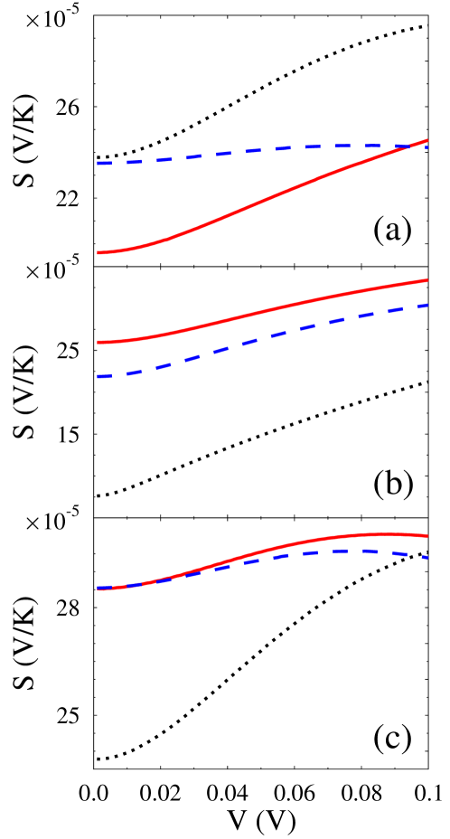
Figure 1: (Color online) Seebeck coefficient vs. applied bias. Shown are results of full self-consistent calculation (solid line, red), scattering theory approach based on model (4) (dashed line, blue), and elastic scattering case (dotted line, black) calculated with (a) ‘standard’ set of parameters (see text for parameters), (b) higher $\varepsilon_{0}-E_{F}$ gap, and (c) weaker electron-phonon coupling $M_{a}$.

Figure 1a shows the Seebeck coefficient $S$ as a function of the bias potential, calculated at $T=300$ K using the energetic parameters $E_{F}=0$, $\varepsilon_{0}=0.2$ eV, $\Gamma_{L}=\Gamma_{R}=0.005$ eV, $\omega_{0}=0.05$ eV, $M_{a}=0.1$ eV, and $\Omega^{ph}_{L}=\Omega^{ph}_{R}=0.005$ eV. The last is a wide-band approximation for molecular vibration broadening (20) due to coupling to thermal baths (for detailed discussion see Ref. [40]). Figures 1b and c show similar results for a higher $\varepsilon_{0}-E_{F}$ gap and a weaker electron-phonon coupling $M_{a}$, respectively. To show the effect of electron-phonon coupling on the Seebeck coefficient we compare the results obtained from the full self-consistent calculation and the scattering theory approximation to the elastic $M_{a}=0$ limit.

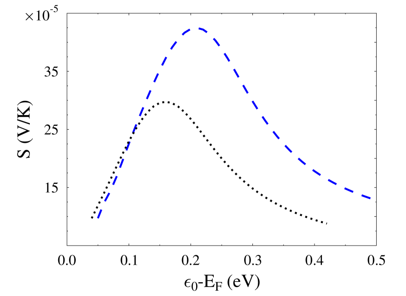
Figure 2: (Color online) Seebeck coefficient vs. energy position of the molecular level for the model of Eq.(4). Shown are results with (dashed line, blue) and without (dotted line, black) electron-phonon interaction. Calculation is done at $V=0.05$ V. Other parameters are the same as in Fig. 1

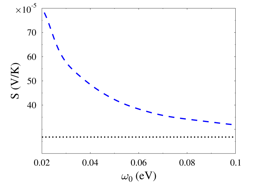
Figure 3: (Color online) Seebeck coefficient vs. vibrational mode frequency for the model of Eq.(4). Shown are result with (dashed line, blue) and without (dotted line, black) electron-phonon interaction. Calculation is done at $V=0.05$ V. Other parameters are the same as in Fig. 1

In the following figures we consider the inelastic effects only within the scattering theory approximation (which requires a far smaller numerical effort). The dependence of $S$ on the energy gap $\varepsilon_{0}-E_{F}$ is shown in Fig. 2, and its variation as function of $\omega_{0}$ is displayed in Fig. 3. In these figures $V$ is kept at the value $0.05$ V and all unvaried parameters are the same as in Fig. 1. Finally, in Fig. 4 we compare self-consistent results (some of them already shown in Fig. 1) obtained for different choices of electron-phonon coupling $M_{a}$ and vibrational broadening $\Omega^{ph}$.

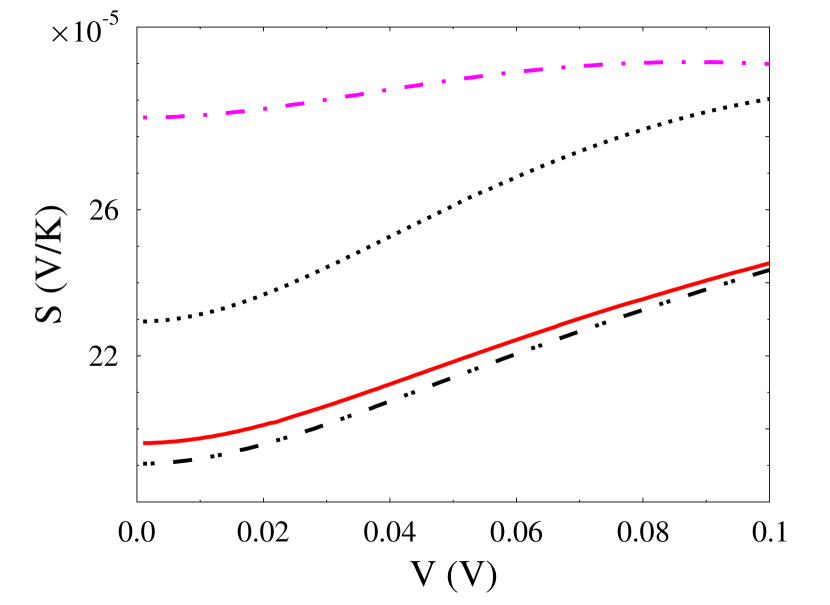
Figure 4: (Color online) Seebeck coefficient vs. applied bias for model described in Section 2. Solid line (red) and dash-dotted line (magenta) are identical to solid lines (red) in Figs. 1a and c respectively. Also shown result for $\Omega^{ph}_{L}=\Omega^{ph}_{R}=0.002$ eV (dash-double dotted line, black). Elastic case (dotted line, black) is shown for comparison.

The following observations can be made regarding these results:

1. In contrast to inelastic tunneling features usually seen in the second derivative $d^{2}I/dV^{2}$ of the current-voltage characteristic near $|eV|=\hbar\omega_{0}$ no such threshold behavior is seen in Fig. 1. This lack of threshold behavior in the inelastic contribution to the Seebeck coefficient results the fact that thermoelectric conduction is assosiated with the tails of the lead Fermi-Dirac distributions, and these tails wash away any thershold structure.

2. Inelastic contributions can have a substantial effect on the Seebeck coefficient and its voltage dependence, however the assessment of these contributions is sensitive to the approximation used and cannot generally be based on the scattering theory level of calculation. Indeed, as seen in Figure 1 $S(V)$ behavior may change qualitatively upon going from the scattering to the self-consistent calculation.

3. Focusing on the self-consistent results, Figs. 1 and 4 show that the inelastic effect on the Seebeck coefficient can be positive or negative, depending on the other energetic parameters in the system. A change of sign as a function of $\varepsilon_{0}$ is seen also in the scattering theory results of Fig. 2. The existence of a similar crossover in the self-consistent results can be inferred by comparing Figures 1a and b.

4. A smaller value of the electron-phonon coupling $M_{a}$ naturally leads to a smaller difference between self-consistent and scattering theory calculations (compare Figs. 1a and c). Still the coupling chosen in Fig. 1c is strong enough to give appreciable difference between the inelastic and elastic results.

5. In Fig. 2 the Seebeck coefficient is seen to go through a maximum as a function of the gap $\varepsilon_{0}-E_{F}$, with inelastic contribution affecting the position and height of the observed peak. The behavior seen in Fig. 2 can be rationalized by noting that for, say, $T_{L}>T_{R}$ electrons with energies $E>E_{F}$ contribute most to left-to-right current, while those with $E<E_{F}$ dominate right-to-left current. This gives no thermoelectric current when $\varepsilon_{0}=E_{F}$, hence as $\varepsilon_{0}\to E_{F}$ one needs a higher temperature difference in order to compensate for the same bias. As a result, the Seebeck coefficient goes down at $\varepsilon_{0}-E_{F}\to 0$. On the other hand when $\varepsilon_{0}-E_{F}\gg\Gamma,k_{B}T$ the two contributions cancel each other, and hence Seebeck coefficient drops down once more.

6. The dependence of $S$ on $\omega_{0}$ (Fig. 3 demonstrates it within a scattering theory level calculation) is in line with the expectation that $S$ should attain its classical limit as the vibration becomes more rigid.

7. We have found (not shown) that effects on $S$ of varying the electronic ($\Gamma$) or vibrational ($\Omega$) widths show a similar trend as varying the gap $\varepsilon_{0}-E_{F}$ or the vibrational frequency $\omega_{0}$, respectively.

5 Conclusion

We studied the influence of molecular vibration (inelastic effects) on the Seebeck coefficient for molecular junction transport using a simple model of one molecular level (representing the participating molecular state) coupled to two contacts and to one molecular vibration. Two approaches to the model were considered: a simplified scattering model represented by Eq.(4) and the full self-consistent approach described in Section 2. The simplified approach ignores the mutual influence of electronic and vibrational subsystems. Note, the structure of the expression for current, Eq.(4) is just a difference between two scattering fluxes (left-to-right minus right-to-left). Results of simplified model calculation are compared to the full self-consistent approach where both mutual electron-vibration influence and vibration coupling to thermal baths are taken into account (for detailed description of the approach see Ref. [29]). We show that inelastic effects have non-negligible influence on the resulting Seebeck coefficient for the junction, for a reasonable choice of parameters. Electron-vibration interaction can either increase or decrease Seebeck coefficient depending on the physical situation. We study the dependence of this influence on different parameters of the model (applied bias, gap between molecular level and Fermi energy, strengths of coupling between molecule and contacts, between tunneling electron and molecular vibration, between molecular vibration coupling and thermal baths, and frequency of the vibration). Comparing results of the two approaches, we show that scattering theory based approach may fail both quantitatively and qualitatively. Experimental data presented in Ref. [24] does not give conclusive evidence for the relative importance of inelastic processes. More extensive measurements showing dependence of the Seebeck coefficient on junction parameters are needed in order to make definite conclusion. In particular, isotopic effects should influence vibration-related part of the Seebeck coefficient (see Figs. 3 and 4). Change in electron-phonon coupling would also reveal the inelastic part of the Seebeck coefficient (see 4). Finally, results of our model calculations done with a reasonable set of parameters provide the Seebeck coefficient to be of the order of $\sim 10^{-4}$ V/K. Results reported in Ref. [24] yield $S\sim 10^{-5}$ V/K. Since molecules used in the experiment[24] are characterized by relatively big gap $\varepsilon_{0}-E_{F}$, our results are in good agreement with the measured data. Indeed, for $\varepsilon_{0}-E_{F}\sim 1$ eV calculated Seebeck coefficient (see Fig. 2) becomes of the experimentally observed order of magnitude.

References

- [1] A. Nitzan and M. A. Ratner, Science 300, 1384 (2003).
- [2] M. A. Reed and T. Lee (Eds.), Molecular Nanoelectronics, American Scientific Publishers, Stevenson Ranch, CA (2003).
- [3] J. M. Tour, Molecular Electronics: Commercial Insights, Chemistry, Devices, Architectures and Programming, World Scientific, River Edge, NJ (2003).
- [4] G. Cuniberti, G. Fagas, and K. Richter (Eds.), Introducing Molecular Electronics, Springer, Berlin (2005).
- [5] K. Schwab, E. A. Henriksen, J. M. Worlock, and M. L. Roukes, Nature 404, 974 (2000).
- [6] P. Kim, L. Shi, A. Majumdar, and P. L. McEuen, Phys. Rev. Lett. 87, 215502 (2001).
- [7] L. Shi and A. Majumdar, Journal of Heat Transfer 124, 329 (2002).
- [8] D. Cahill, K. Goodson, and A. Majumdar, Journal of Heat Transfer 124, 223 (2002).
- [9] N. Agrait, C. Untiedt, G. Rubio-Bollinger, and S. Vieira, Phys. Rev. Lett. 88, 216803 (2002).
- [10] D. Cahill, W. K. Ford, K. E. Goodson, G. D. Mahan, A. Majumdar, H. J. Maris, R. Merlin, and S. R. Phillpot, J. Appl. Phys. 93, 793 (2003).
- [11] M. J. Montgomery, T. N. Todorov, and A. P. Sutton, J Phys.: Cond. Matter 14, 5377 (2002).
- [12] B. N. J. Persson and P. Avouris, Surface Science 390, 45 (1997).
- [13] A. P. van Gelder, A. G. M. Jansen, and P. Wyder, Phys. Rev. B 22, 1515 (1980).
- [14] A. Cummings, M. Osman, D. Srivastava, and M. Menon, Phys. Rev. B 70, 115405 (2004).
- [15] I. Paul and G. Kotliar, Phys. Rev. B 67, 115131 (2003).
- [16] D. Segal, A. Nitzan, and P. Hanggi, J. Chem. Phys. 119, 6840 (2003).
- [17] D. Segal and A. Nitzan, Phys. Rev. Lett. 94, 034301 (2005).
- [18] D. Segal and A. Nitzan, J. Chem. Phys. 122, 194704 (2005).
- [19] K. R. Patton and M. R. Geller, Phys. Rev. B 64, 155320 (2001).
- [20] Y. C. Chen, M. Zwolak, and M. Di Ventra, Nano Lett. 3, 1691 (2003).
- [21] M. Galperin, M. A. Ratner, and A. Nitzan, J. Phys.: Condens. Matter 19, 103201 (2007).
- [22] M. Galperin, A. Nitzan, and M. A. Ratner, Phys. Rev. B 75, 155312 (2007).
- [23] J. C. Poller, R. M. Zimmermann, and E. C. Cox, Langmuir 11, 2689 (1995).
- [24] P. Reddy, S.-Y. Jang, R. A. Segalman, and A. Majumdar, Science 315, 1568 (2007).
- [25] M. Paulsson and S. Datta, Phys. Rev. B 67, 241403(R) (2003).
- [26] E. Macia, Nanotechnology 16, S254 (2005).
- [27] D. Segal, Phys. Rev. B 72, 165426 (2005).
- [28] K. Walczak, Physica B 392, 173 (2007).
- [29] M. Galperin, A. Nitzan, and M. A. Ratner, Phys. Rev. B 73, 045314 (2006).
- [30] B. J. LeRoy, S. G. Lemay, J. Kong, and C. Dekker, Nature 432, 371 (2004).
- [31] A. Mitra, I. Aleiner, and A. J. Millis, Phys. Rev. B 69, 245302 (2004).
- [32] G. D. Mahan, Many-Particle Physics. (Third edition, Kluwer Academic/Plenum Publishers, New York, 2000).
- [33] I. G. Lang and Yu. A. Firsov, Sov. Phys. JETP 16, 1301 (1963).
-
[34]
Y. Meir and N. S. Wingreen,
Phys. Rev. Lett. 68, 2512 (1992);
A. Jauho, N. S. Wingreen, and Y. Meir, Phys. Rev. B 50, 5528 (1994). - [35] H. Haug and A.-P. Jauho, Quantum Kinetics in Transport and Optics of Semiconductors, Springer, Berlin (1996).
- [36] P.N.Butcher, J. Phys.: Cond. Matter 2, 4869 (1990).
- [37] L.D.Landau and E.M.Lifshitz, Statistical Physics, Part 1, Pergamon Press, London (1968).
- [38] M.Abramowitz and I.A.Stegun, Eds., Handbook of mathematical functions with formulas, graphs, and mathematical tables, Dover Publications, New York (1964).
-
[39]
To obtain Eq.(4) from Eq.(13)
the ”first iterative step” of the self consistent procedure[29]
has to be taken. This leads to (see Eq.(2))
In order to keep the the symmetry for the current expression, one has to introduce the second FC factor in the Keldysh equation for
Substituting these expressions into Eq.(13) and expanding FC factors in term of Bessel functions leads to Eq.(4). - [40] M.Galperin, M.A.Ratner, and A.Nitzan, J. Chem. Phys. 121, 11965 (2004).