Locally Adaptive Nonparametric Binary Regression

Abstract

A nonparametric and locally adaptive Bayesian estimator is proposed for estimating a binary regression. Flexibility is obtained by modeling the binary regression as a mixture of probit regressions with the argument of each probit regression having a thin plate spline prior with its own smoothing parameter and with the mixture weights depending on the covariates. The estimator is compared to a single spline estimator and to a recently proposed locally adaptive estimator. The methodology is illustrated by applying it to both simulated and real examples.
KEY WORDS: Bayesian analysis; Markov chain Monte Carlo; Mixture-of-Experts; Model averaging; Surface Estimation; Reversible jump;

1 Introduction

Suppose we wish to model the spatial distribution of the habitat of the crested lark. One way to do this is to model the probability of a crested lark sighting as a function of latitude ($lat$) and longitude ($lon$) as

$$\Pr(\mbox{crested lark sighting}|lat,lon) =H\left\{g(lat,lon)\right\},$$ (1.1)

where $H$ is a link function, such as a probit or logit, and $g$ is a function of latitude and longitude, which is either parametric or nonparametric. Our article presents a Bayesian method for estimating the probability in (1.1) that does not assume a parametric form for $H$ and allows the probability to be locally adaptive with respect to the covariates, that is, to be smooth in one region of the covariate space and wiggly or even discontinuous in another.

We model the binary regression as a mixture of probit binary regressions

$$\Pr(\text{crested lark sighting}|Lat,Lon) =\sum_{j=1}^{r}\pi_{j}(Lat,Lon)\Phi\left\{g_{j}(Lat,Lon)\right\}\ ,$$ (1.2)

where $\Phi$ is the standard normal cumulative distribution function and the $g_{j}$ are truncated spline functions. We demonstrate that the resulting estimators are nonparametric and locally adaptive, but do not overfit. The reasons for this good performance are that mixing is done outside the probit cumulative distribution function rather than inside, the weights $\pi_{j}$ are allowed to vary with the covariates, and that the component functions $g_{j}$ can have different level of smoothness by having different smoothing parameters. This is especially important when modeling surfaces in two or more dimensions where a single smoothing parameter for a multidimensional surface will often be inadequate. The use of truncated spline bases allows models with several thousand observations and regression surfaces with a moderate number (at least 6 or 7) of covariates (provided the number of observations is adequate). Extending the methodology to higher dimensions problems is important because as the number of covariates increase so too does the need for local smoothing. This is because the smoothness of the function $H(x)$ is likely to be different for different covariates. Our article allows the number of components to vary from $r=1,\dots,R$, with $R$ typically 3 or 4. We use a Bayesian approach and construct a Markov chain Monte Carlo sampling scheme (MCMC) to estimate the model that uses the reversible jump method of Green (1995) to move between model spaces having different numbers of components.

Model (1.2) is known as a Mixture-of-Experts (ME) model and was first introduced by Jacobs et al. (1991) and Jordan and Jacobs (1994), who used simple linear functions for the $g_{j}$ and estimated the model by the EM algorithm.

There is an extensive literature on estimating binary regressions. McCullagh and Nelder (1989) discuss parametric approaches. Nonparametric binary regression is discussed by Wang (1994, 1997), Wahba, Wang, Gu, Klein and Klein (1997) and Loader (1999). Wood and Kohn (1998) and Holmes and Mallick (2003) present Bayesian approaches to nonparametric binary regression. However, none of these papers show that their estimates are locally adaptive. Kribovokova et al. (2006) present an estimator of a binary regression that is based on quasi likelihood and show that it is locally adaptive.

A number of locally adaptive estimators have recently been proposed for Gaussian regression models. Most of these estimators represent the unknown regression function as a linear combination of basis functions. Frequentist approaches such as Friedman and Silverman (1989), Friedman (1991) and Luo and Wahba (1997) sought an optimal combination of basis functions using a greedy search algorithm, whereas Bayesian approaches such as Smith and Kohn (1996) and Denison, Mallick and Smith (1998) averaged over a large number of combinations of subsets of the basis functions.

Wood, Jiang and Tanner (2002) proposed a locally adaptive estimator for Gaussian regression by mixing over a combination of splines and used BIC to choose the number of components. Our article builds on this Mixture of Experts approach by Wood,et al. (2002).

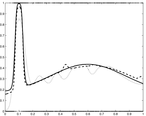
A direct way to obtain a locally adaptive estimator of binary probabilities is to adaptively estimate $g$ in (1.1) by using latent variables together with the basis selection methods in Friedman (1991), Denison, Mallick and Smith (1998), and Smith and Kohn (1996) or with the mixture of splines method in Wood et al. (2002). However, we have found that for the mixture of splines approach, adaptively estimating the regression function $g$ by mixing on the inside of $\Phi$ results in poor estimates of the probabilities due to overfitting. Figure 1 gives an example of such overfitting. The figure shows the true probability $H(x)=Pr(y=1|x)$ and the estimate $\widehat{H}(x)=\Phi(\widehat{g}(x))$ where $g(x)=\pi(x)f_{1}(x)+(1-\pi(x))f_{2}(x)$, which we call mixing on the inside. The figure also shows the estimate of $H(x)$ based on modeling $H(x)$ as $\pi(x)\Phi\{f_{1}(x)\}+(1-\pi(x))\Phi\{f_{2}(x)\}$, which we call mixing on the outside. In this example, which is typical of all such examples, it is clear that mixing on the inside does not perform as well as mixing on the outside. The technical report by Wood, Kohn, Jiang and Tanner (2005) provides details of why mixing on the inside tends to result in overfitting and produces inferior estimates to mixing on the outside.

2 Model and Prior Specification

We present the model in this section. Appendix A gives details of the sampling scheme used to estimate the model. Using the results in Tierney (1994) and Green (1995) we can show that the sampling scheme converges to the posterior distribution.

Let $w$ be a binary response variable taking the values 0 and 1. We model the binary regression of $w$ on $x$ by a mixture of finite but unknown number of probit regressions, as

$$\Pr(w=1|x) =\sum_{r=1}^{R}H_{r}(x)\Pr(r)\ ,\text{ }H_{r}(x)=\sum_{j=1}^{r}\pi_{jr}(x)\Phi\{g_{jr}(x)\}$$ (2.1)

$$\text{with}\quad\pi_{jr}(x) =\exp(\delta_{jr}^{\prime}z)/\sum_{k=1}^{r}\exp(\delta_{kr}^{\prime}z)\ ,j=1,\dots,r,$$

where $z=(1,x^{\prime})^{\prime}$. We usually take the number of components $R$ as 3 or 4 with $\Pr(r)=1/R$, for $r=1,\dots,R$. Without loss of generality we assume that the vector $\delta_{1r}=0$ and let $\delta_{r}=(\delta_{2r},\dots,\delta_{rr})$ be a vector of unconstrained coefficients. We observe $w_{1},\dots,w_{n}$ as well as the corresponding covariates $x_{1},\dots,x_{n}$.

To place a prior on $g_{jr}$ we write

$$g_{jr}(x) =\alpha_{jr}^{\prime}z+f_{jr}(x)$$ (2.2)

where $\alpha_{jr}$ is a coefficient vector and $f_{jr}(x)$ is the nonlinear part of $g_{jr}$. For $j=1,\dots,r$, let ${\bf{f}}_{jr}=\biggl{(}f_{jr}(x_{1}),\dots,f_{jr}(x_{n})\biggr{)}^{\prime}$. We write ${\bf{f}}_{jr}$ as a linear combination of basis functions as outlined below so that ${\bf{f}}_{jr}=X\beta_{jr}$, where the columns of the design matrix $X$ are partial thin plate spline basis functions and $\beta_{jr}$ is a vector of coefficients. Appendix B describes how we construct the design matrix $X$ to handle a large number of observations $n$ and a moderate number of covariates.

The prior for $\alpha_{jr}$ for $j=1,\ldots,r$ is $N(0,c_{\alpha}I)$, for some large $c_{\alpha}$, and we assume that the $g_{jr}$’s are independent apriori. Based on emprical evidence we found that the regression function estimates were insensitive to the choice of $c_{\alpha}$ over the range $[10^{2},10^{10}]$. The prior for $\beta_{jr}\sim N(0,\tau_{jr}I),j=1,\dots,r$. We assume a uniform prior for $\tau_{1r}\sim U(0,c_{\tau})$, for some large $c_{\tau}$ . To ensure identifiability we assume apriori that $\tau_{jr}\sim U(0,\tau_{(j-1)r})$ for $j=2,\ldots,r$, i.e., $\tau_{1r}<,\ldots,<\tau_{rr}<c_{\tau}$. The prior on the parameter vector $\delta_{r}$ for the mixing probabilities is $N(0,c_{\delta}I))$, where $c_{\delta}=n$.

3 Simulations

3.1 Comparison with a single component estimator

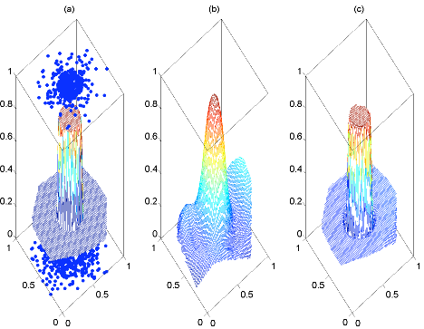
The performance of the proposed method is studied for four functions listed in table 1, using a sample size of $n=1000$ for each function. The three univariate functions are plotted in Figure 3. The bivariate function is plotted in Figure 4(a). The four functions are chosen in such a way that each requires a different type of smoothing. Function (a) requires only one smoothing parameter, function (b) requires local smoothing, function (c) is a discontinuous function, and function (d) is a discontinuous bivariate function.

Function Label	Function Formula
a (sin)	$\Pr(w=1|x)=\Phi\{2\sin(4\pi x)\}$
b (peak)	$\Pr(w=1|x)=\Phi\{\frac{5}{6}\exp{\left[\frac{(x-0.1)^{2}}{0.18}\right]}+\frac{1}{3}\exp{\left[\frac{(x-0.6)^{2}}{0.004}\right]}-1\}$
c (step)	$\Pr(w=1|x)=\Phi\{-1.036+2.073I_{x}(0.25)-1.42712I_{x}(0.75)\}$
	where $I_{x}(a)=1$ if $x>a$
d (cylinder)	$\Pr(w=1|x)=D\{(x-0.5)^{2}+(y-0.5)^{2}-0.16^{2}\}$
	where $D(x)=0.8$ if $x<0$ and $D(x)=0.2$ if $x>0$

Table 1: Regression functions used in simulations

The estimates obtained using the proposed method are compared to estimates obtained using a single component estimator as in Wood and Kohn (1998). We use this estimator for comparison because Wood and Kohn (1998) show that their single spline estimator outperforms other available estimators, such as GRKPACK by Wang (1997). Fifty replications were generated for each regression function using a maximum $R=3$ components. We use the average symmetric Kullback-Leibler distance to measure performance. This measure is also used by Gu (1992) and Wang (1994), and is defined below. Let

$$I\{H(x_{i}),{\widehat{H}}(x_{i})\}={{\widehat{\Pr}}}(w_{i}=0|x_{i})\log\left\{\frac{{{\widehat{\Pr}}}(w_{i}=0|x_{i})}{Pr(w_{i}=0|x_{i})}\right\}+{{\widehat{\Pr}}}(w_{i}=1|x_{i})\log\left\{\frac{{{\widehat{\Pr}}}(w_{i}=1|x_{i})}{\Pr(w_{i}=1|x_{i})}\right\}\,.$$

By Rao (1973, pp. 58-59), $I\{H(x_{i}),\hat{H}(x_{i})\}\leq 0$ and $I\{H(x_{i}),{{\widehat{H}}}(x_{i})\}=0$ if and only if $H(x_{i})={{\widehat{H}}}(x_{i})$ at the design points. The average symmetric Kullback-Leibler distance (ASKLD) between $H$ and ${\widehat{H}}$ is defined as

$$ASKLD(H,{\widehat{H}})=\frac{1}{n}\sum_{i=1}^{n}\left[I\{H(x_{i}),{\widehat{H}}(x_{i})\}+I\{{\widehat{H}}(x_{i}),H(x_{i})\}\right]\,.$$

It follows from the properties of the Kullback-Leibler distance that $ASKLD(H,{\widehat{H}})\leq 0$ and $ASKLD(H,\hat{H})=0$ if and only if ${\widehat{H}}=H$. Thus, the closer $I(H,{\widehat{H}})$ is to zero the better.

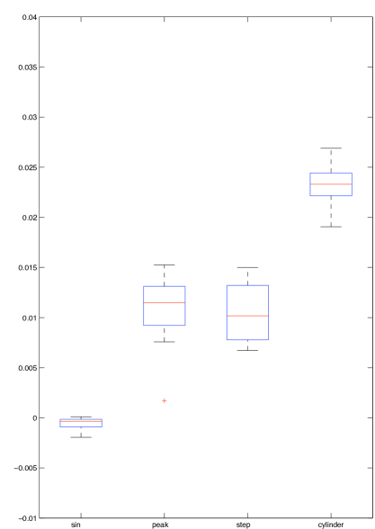
For each replication, the ASKLD was calculated for both estimators, where ${\widehat{H}}(x_{i})$ is the estimate obtained for the function $Pr(w_{i}=1|x_{i})$. Figure 2 compares the performance of the mixture estimator with the performance of the single component estimator using boxplots, with each boxplot representing the average difference in ASKLD for the fifty replications for that function. A positive difference means that the mixture model performs better than the single spline estimator for that replication, while a positive difference means the opposite.

Figure 2 shows that the mixture of splines estimator performs significantly better in terms of the ASKLD than the single spline estimator when the regression surface is heterogenous, that is when it requires local smoothing. In particular, for the heterogeneous functions (b), (c) and (d) the mixture estimator outperformed the single spline. Furthermore, when the function is homogenous, that is when it does not require local smoothing, the mixture estimator performs almost as well as a single spline estimator because when only one spline is needed, for example for function (a), the posterior probability of a single spline is high.

Table 2 gives the average (over the 50 replications) posterior probability of the number of splines needed for mixing for each of the four regression functions. The table shows that for the homogenous function (a) the average posterior probability that only one spline is need is 0.78. In general we have found that for homogenous functions the posterior probability of a single component is high. Conversely, we have found that for heterogenous functions the posterior probability of requiring more than a single component is high. Thus, for function (b), the average posterior probability is 0.76 that two splines are needed and 0.24 that three spline are needed. For the piecewise constant functions (c) and (d), the average posterior probabilities that two splines are needed are 0.60 and 0.84 respectively, whereas the average posterior probabilities that three splines are need is 0.37 and 0.08 respectively.

Function Label	$\Pr(r|\mbox{\boldmath$w$})$
	$1$	$2$	$3$
a (sin)	$0.78$	$0.21$	$0.01$
b (peak)	$0.00$	$0.76$	$0.24$
c (step)	$0.03$	$0.60$	$0.37$
d (cylinder)	$0.08$	$0.84$	$0.08$

Table 2: Average posterior probability of number of splines needed

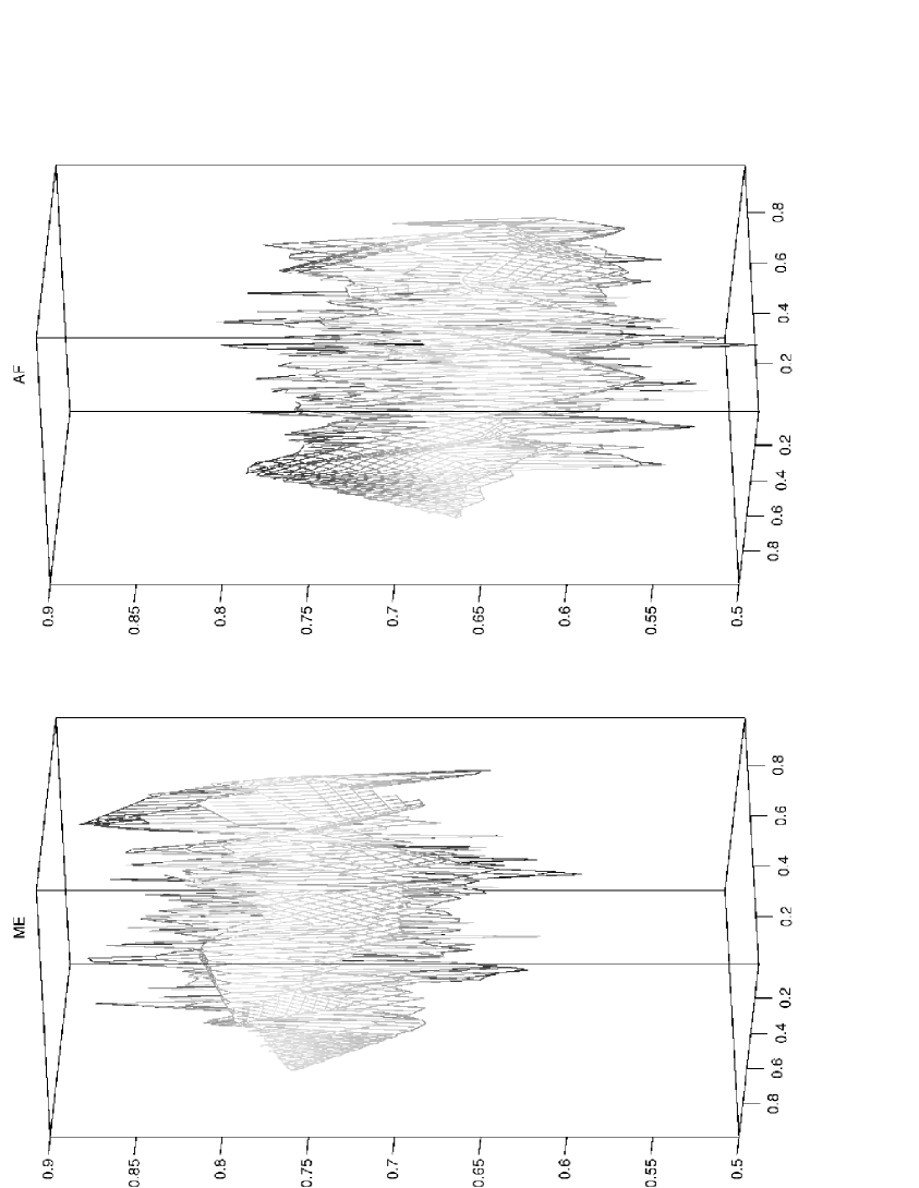
To see how the difference in ASKLD translates into differences in the regression function estimates, the estimates for functions (a)-(c) corresponding to the 10th percentile, 50th percentile and 90th percentile ASKLD are plotted in Figure 3. Figure 3 shows that an estimator based on a mixture of splines can accurately estimate both homogeneous and heterogeneous functions. When the function is homogeneous, e.g. function (a), the mixture estimates are visually indistinguishable from the single spline estimates. However, when the function is heterogeneous, the single spline estimates are much worse than the mixture estimates. For example, even the $90^{th}$ percentile of the single spline estimate of function (b) fails to capture the peak on the left and overfits on the right, whereas the mixture estimate does well throughout the whole range of the function. Figure 4 plots the fit for the cylinder data for a single spline and a mixture of splines. The improvement is marked, with the single spline being unable to capture the sudden change of curvature.

3.2 Comparison to a locally adaptive estimator

Kribovokova et al. (2006) propose a general approach for locally adaptive smoothing in regression models with the regression function modeled as a penalized spline that has a smoothly varying smoothing parameter function which is also modeled as a penalized spline. In particular, their approach handles local smoothing of binary data. The authors have implemented their approach in a package called Adaptfit which is written in R and is available at http://cran.r-project.org/src/contrib/Descriptions/AdaptFit.html. This section compares our approach to that of Kribovokova et al. (2006) as implemented in Adaptfit in terms average squared error, coverage probabilities and running time for the four functions (a)–(d). The results reported below are each based on 50 replications unless stated otherwise.

Let $\text{ASE}_{ME}$ be the average squared error over the abcissae of the data of the Bayesian ME estimator and let $\text{ASE}_{AF}$ be the corresponding averaged squared error of the Adaptfit estimator. We define the percentage change in going from the ME estimator to the adaptfit estimator as

$$\%\Delta\text{ASE} =\frac{ASE_{AF}-ASE_{ME}}{ASE_{ME}}\times 100\ .$$

Table 3 reports the 25th, 50th, 75th percentiles and the mean of $\%\Delta\text{ASE}$ and shows that the ME estimator and the Adaptfit estimator perform similarly for functions (a) and (b), but that the ME of experts estimator outperforms the Adaptfit estimator for functions (c) and (d).

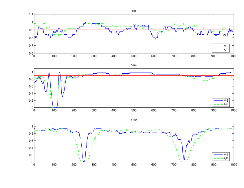
Let the empirical coverage probability $\text{ECP}_{ME}(x)$ be the proportion (out of 50) of 90% pointwise confidence intervals that contain the true probability at the abcissa $x$ for the ME estimator. Let $\text{ECP}_{AF}(x)$ be defined similarly for the Adaptfit estimator. Figure 5 plots $\text{ECP}_{ME}(x_{i})$ and $\text{ECP}_{AF}(x_{i})$ at the abcissae $x_{i}$ of the data for the functions (a)–(c). Figure 6 is a similar plot for the cylinder function (d). Let

$$\%\Delta\text{AECP}_{ME} =100\times\biggl{(}n^{-1}\sum_{i=1}^{n}\text{ECP}_{ME}(x_{i})-0.9\biggr{)}/0.9$$

be the percentage deviation from 0.9 of the average of the $\text{ECP}_{ME}(x_{i})$ over all the $x_{i}$ abcissae of the data. Let $\%\Delta\text{AECP}_{AF}$ be defined similarly for the Adaptfit estimator. Table 3 reports both $\%\Delta\text{AECP}_{ME}$ and $\%\Delta\text{AECP}_{AF}$. Figure 5 and table 3 suggest that the empirical coverage probabilities of the ME estimator and Adaptfit are similar for functions (a) and (b), while the ME estimator has superior empirical coverage probabilities for functions (c) and (d).

Function	$\%\Delta\text{ASE}$				$\%\Delta\text{AECP}$
	25	50	75	mean	ME	AF
(a) Sin	$-11.32$	$7.86$	$29.64$	$11.18$	$-0.74$	$3.10$
(b) Peaks	$-8.03$	$-0.703$	$15.07$	$7.72$	$-3.34$	$-5.89$
(c) Step	$52.23$	$93.15$	$140.23$	$101.99$	$-9.07$	$-18.12$
(d) Cylinder	$86.28$	$130.76$	$162.11$	$126.83$	$-16.80$	$-26.62$

Table 3: Comparison of Bayesian ME and adaptfit. The first four columns give the 25th, 50th , 75th percentiles and the mean of the percentage difference between the averaged mean squared error of adaptfit and the ME estimators. The next two columns gives the percentage coverage errors of the 90% confidence intervals for ME and Adaptfit.

We now discuss some computational issues that determine the performance of Adaptfit in the binary regression case. Adaptfit uses two sets of knots. The first set of knots is for the penalized spline basis for the regression function and the second set of knots is for the penalized spline basis for the smoothing parameters. See Kribovokova et al. (2006) for details. Let $K_{b}$ be the number of knots chosen for the first penalized spline and $K_{c}$ the number of knots chosen for the second penalized spline. We found in the binary case that if a function requires a locally adaptive estimator then to get a satisfactory fit it may be necessary to take $K_{b}$ quite large. For example, for the peak function (b) and the cylinder function (d) it seems necessary to take $K_{b}=120$ to 150. The results for functions (a), (c) and (d) in table 3 were obtained using using $K_{b}=150$ and $K_{c}=20$. The results for function (b) (peak) were supplied to us by Dr Tatyana Krivobokova who used an Splus implementation of Adaptfit because we were unsuccessful with the R implementation . The results reported for Adaptfit for function (b) are for 47 replicates with the other three replicates being unsatisfactory. Adaptfit also has a default choice of $K_{b}$ and $K_{c}$ and we checked that the above settings for functions (a), (c) and (d) gave as good or better performance as the defaults. The times given below are averages over several replications and were obtained on a 2.8GHz PC running Matlab 7. For function (a), Adaptfit took 25 seconds for the default number of knots and 320 seconds for $(K_{b},K_{c})=(150,20)$. For function (c), Adaptfit took 36 seconds for the default number of knots and 325 seconds for $(K_{b},K_{c})=(150,20)$. For function (d), Adaptfit did not give satisfactory results for the default number of knots and took 316 seconds for $(K_{b},K_{c})=(150,20)$. The ME estimator takes about 90 seconds per 2000 iterations for each of the examples in this section. For each of the examples reported in this section and the next section we ran the ME estimator for 10000 iterations in total (5000 warmup and 5000 sampling), that is, the time taken for each of the examples in this section is about 450 seconds. However, we have found in extensive testing that it is sufficient to use 4000 to 6000 iterations in all of these examples, that is about 180 to 270 seconds in total. All the times reported were recorded on a 2.8GHz PC running Matlab 7. Thus Adaptfit can be very fast when the default number of knots is used, but for a binary regression it is difficult to determine apriori for any data set whether the default number of knots is adequate and in our opinion it is safer to take the more conservative approach by setting $K_{b}$ to 120 or 150. In that case the times required by Adaptfit and the ME estimators are not that different, while the ME estimator in the binary case appears computationally more robust.

4 Real Examples

4.1 Probability of crested lark sighting in Portugal

This section demonstrates how the proposed method can be used to model spatial data by modelling the probability of a crested lark sighting at various locations in Portugual. The data were obtained from Wood (2006). Each observation refers to one tetrad (2km by 2km square) and contains a variable indicating whether the crested lark was sighted in the tetrad or not together with the location of the tetrad. The location of a tetrad is identified by kilometers east and north of an origin. Portugal can be divided into 25100 tetrads for which there were observations on 6457 tetrads. This dataset was analysed by Wood (2006) who aggregated the data into 10km by 10km squares and fitted a binomial generalized additive model (GAM) using thin plate regression splines to the aggregated response. In their example the degree of smoothness was estimated using the un-biased risk estimator (UBRE), which was then scaled-up by a factor of 1.4 to avoid overfitting. The factor by which the smoothing parameter is rescaled is chosen subjectively and affects the estimated probabilities substantially. In contrast, our method allows for the degree of smoothness to vary across the covariate space and the estimated probabilities are therefore spatially adaptive .

Our model for the probability of a crested lark sighting is given by (2.1) and (2.2) with $x=(east,north)$, where $east$ and $north$ mean kilometers east and north of an origin. The dependent variable is 1 if a crested lark is sighted in a tetrad and 0 if it is not. We assume a maximum of four mixture components.

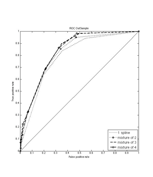
We considered the choice of the number of mixture components in several ways. First, the posterior probabilities for 1 to 4 components are 0.0, 0.94, 0.04 and 0.01, suggesting a two component mixture. We also looked at the empirical receiver operating curves (ROC) for models with 1 to 4 components. See Fan, Upadhye and Worster (2006) for a description of ROC curves. In our case a ROC curve shows the trade off between classifying a tetrad as containing the crested lark when the tetrad does contain the crested lark versus classifying a tetrad as containing the crested lark when it does not. The larger the area under the ROC curve the more effective is the model at classifying. Out of 6457 observations we randomly selected 5817 for model fitting and set aside 640 for model testing. We estimated the probability that a tetrad contains the crested lark using mixture models containing one to four components. For each mixture model we then used the estimated probabilities to classify the 640 observations set aside for model testing. Figure 7 plots the empirical ROC curves based on these 640 observations and shows the improvement in classification that is achieved by using a mixture of two splines over a single spline. Figure 7 also shows that there is not much improvement in classification in moving from a mixture of two to a mixture of three or four and hence supports the choice of a mixture of two splines as the preferred model. This finding is consistent with the posterior probabilities of the number of components.

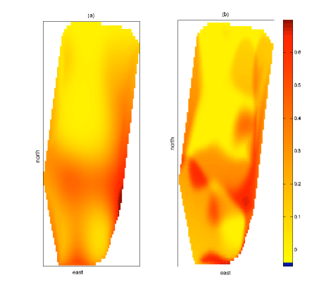
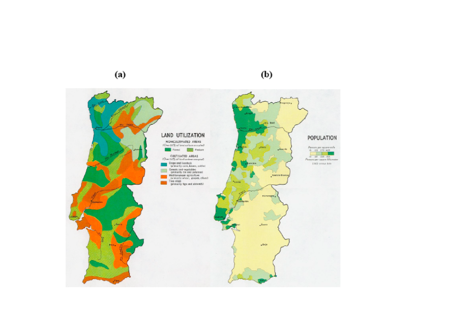
Figure  8 shows contour plots for the probability of a crested lark sighting for a single spline estimator and a mixture of splines estimators. This figure and the land use and population maps, reproduced in figure, 9 show why a mixture of at least 2 splines is necessary. Mainland Portugal is split by the river Tagus. The population and land use maps show that the population of Portugal is concentrated to the north of the river, in particular in the northwest where the land is given over to wine production. The interior of the north is dry and mountainous. To the south of the river the predominant land form is rolling hills and the area is much less densely populated. The cultivated areas in the south are primarly for cork production but there are large tracts of forested areas.

Figure 8(b) shows that in the southern part of Portugal the probability of sighting a crested lark varies considerably and that these variations can occur abruptly. These abrupt changes correspond to changes in the topography of southern Portugal. The areas of high probability correspond to forested/tree crop areas or major rivers. The areas of low probability correspond to pasturable lands. In contrast the probability of a crested lark sighting in the northern part of Portugal has little variation; the high population density together with the mountainous interior means that the probability is of sighting is uniformly low. Thus the degree of smoothing required depends on the covariates $east$ and $north$. Figure 8 (a) shows that a single spline estimator cannot simultaneously capture the abrupt changes in southern Portugal and the smooth changes in the north.

4.2 Probability of belonging to a union

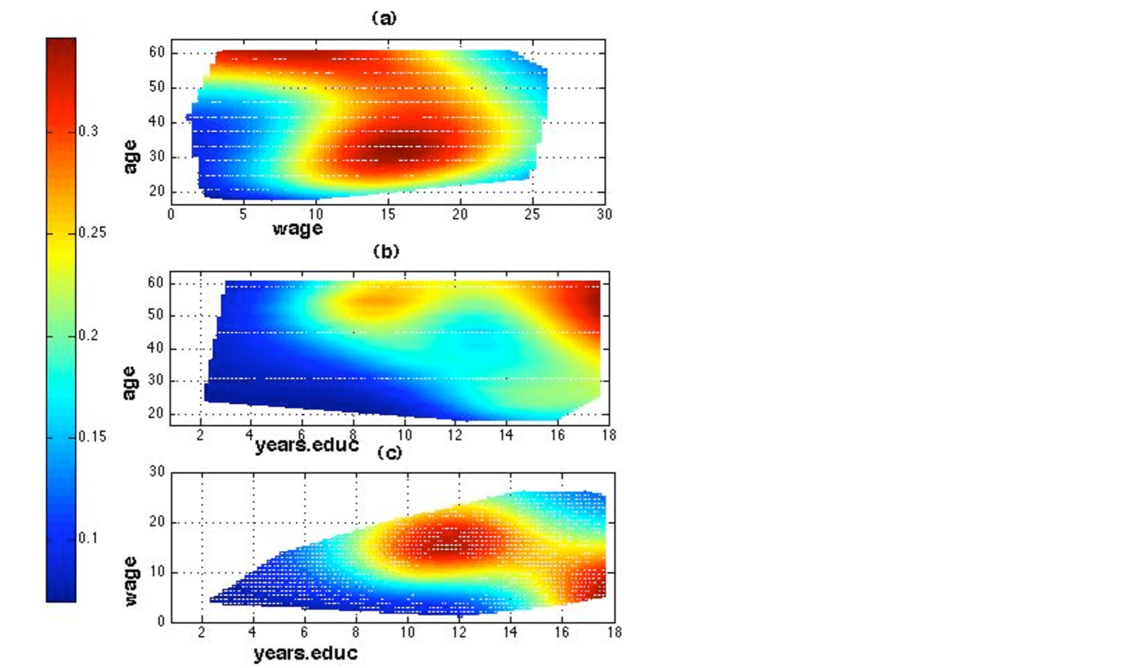
This example shows how our methodology can be extended higher dimensions by modeling the probability of union membership as a function of three continuous variables, years education, wage and age, and three dummy variables, south (1=live in southern region of USA), female (1=female) and married (1=married). The data consists of 534 observations on US workers and can be found in Berndt (1991) and at http://lib.stat.cmu.edu/datasets/CPS_85_Wages. Ruppert, Wand and Carroll (2003) estimate the probability of union membership using a generalized additive model without interactions. We model the three dimensional surface of the continuous covariates and our results suggest that this more appropriate than an additive model. Our model for the probability of union membership is given by (2.1) with $x=$(years education, wage, age, south, female, married). However, we modify the regression function (2.2) to take into account that three of the covariates are dummy variables and should be excluded from the non-parametric component by writing

$$g_{jr}(x) =\alpha_{jr}^{\prime}z+f_{jr}(x^{*})$$

where $x^{*}=$ (years education, wage, age), wage is in US $/hr and age is in years. The dependent variable is 1 if the worker belongs to a union and 0 otherwise.

Our method chooses one component 100% of the time. Figures  10 (a) - (c) show the joint marginal effect of two covariates at the mean of the third one and setting the dummy variables to zero. These figures clearly show interactions among the continuous covariates. For example figure  10 (a) shows that for workers whose age is less than 40, the probability of union membership initially increases with $wage$, before reaching a peak at a wage of about $\$15/hr$ and then declines. For older workers this peak occurs at much lower wages, somewhere between $\$5$/hr and $\$10$/hr before declining sharply. Figure 10 (b) shows two modes. For workers with an average wage, union membership peaks at 55 years and 8-10 years education. Interestingly union membership peaks again at 55 years and 18 years education, although this peak may be due to boundary effects. Figure  10 (c) shows that for workers who did not finish high school ($<12$ years education) the probability of belonging to union increases as wage increases. In contrast, for workers with some tertiary education($>14$ years education) the probability of belonging to a union is initially high and then decreases with increasing wage.

Appendix Appendix A: Sampling scheme

We estimate the binary regression probabilities by their posterior means, with all unknown parameters and latent variables integrated out. To make it easier to simulate from the posterior distribution we introduce a number of latent variables that are generated during the simulation and turn (2.1) into a hierarchical model. The first is the number of components $r$ at any point in the simulation. Given $r$, define the vector of multinomial random variables $\mbox{\boldmath$\gamma$}_{r}=\left\{{\gamma_{r}(x_{1}),\ldots,\gamma_{r}(x_{n})}\right\}$ such that $\gamma_{r}(x_{i})$ identifies the component in the mixture that $w_{i}$ belongs to. We assume that

$$\Pr(\mbox{\boldmath$\gamma$}_{r}|r,\mbox{\boldmath$\delta$}_{r},x) =\prod_{i=1}^{n}\Pr\{\gamma_{r}(x_{i})|r,\mbox{\boldmath$\delta$}_{r},x\}\ ,\quad\text{with}\quad\Pr\{{\gamma_{r}(x_{i})=j|\mbox{\boldmath$\delta$}_{r}}\}=\pi_{jr}(x_{i})\quad\text{and}$$

$$\Pr(\mbox{\boldmath$w$}|r,\mbox{\boldmath$\gamma$}_{r},\mbox{\boldmath$g$}_{r}) =\prod_{i=1}^{n}\Pr\{w_{i}|\gamma_{r}(x_{i})=j,g_{jr}(x_{i})\}$$

To estimate the component splines, we follow Albert and Chib (1993) and Wood and Kohn (1998) and introduce a second level of latent variables, $v_{ijr}$, also conditional on $r$, such that

$$v_{ijr}=z_{i}\alpha_{jr}+f_{jr}(x_{i})+\epsilon_{ijr}\quad\mbox{for}\quad j=1,\ldots,r\quad\mbox{and}\quad i=1,\ldots,n,$$

where $\epsilon_{ijr}\sim N(0,1)$. The latent variable $v_{jir}$ and the indicator variable $\gamma_{r}(x_{i})$ are related to each other and the observation $w_{i}$ by requiring that

$$\begin{array}[]{lcrllcrllcl}v_{ijr}&>&0&\mbox{if}&w_{i}&=&1&\mbox{and}&\gamma_{r}(x_{i})&=&j\\ v_{ijr}&<&0&\mbox{if}&w_{i}&=&0&\mbox{and}&\gamma_{r}(x_{i})&=&j.\end{array}$$

If $\gamma_{r}(x_{i})\neq j$, then $v_{ijr}$ is unconstrained.

The sampling scheme moves between models with differing numbers of components by using reversible jump MCMC. To implement a reversible jump step to go from a model with $r$ components to a model with $r^{\prime}$ components it is necessary to have a proposal density in the $r^{\prime}$ component space. We form such proposals by first running separate MCMC samplers for each $r=1,\dots,R$ component models. This sampling scheme is described below under the heading of ‘Updating within a model.’

We now describe the complete sampling scheme. First, $r$ is initialized by drawing it from the prior $\Pr(r=j)=1/R,j=1,\dots,r$. Conditional on this value of $r$, we initialize $\mbox{\boldmath$\beta$}_{r}$, $\mbox{\boldmath$\alpha$}_{r}$,$\mbox{\boldmath$\tau$}_{r}$, $\mbox{\boldmath$\delta$}_{r}$ by the posterior means of the iterates of the model with $r$ components.

1. Moving Between Models
   Let $X^{c}=(r^{c},\Theta_{r}^{c})$ be the current value of the parameters in the chain, where $\Theta_{r}^{c}=(\mbox{\boldmath$\alpha$}_{r}^{c},\mbox{\boldmath$\beta$}_{r}^{c},\mbox{\boldmath$\delta$}_{r}^{c})$. We propose a new value of $X^{p}=(r^{p},\Theta_{r}^{p})$ and accept this proposal using a Metropolis-Hastings (M-H) step. The M-H probability of accepting such a proposal is

   $$\epsilon(X^{c},X^{p}) = \min\left\{1,\frac{p(X^{p}|\mbox{\boldmath$w$})q(X^{p},X^{c})}{p(X^{c}|\mbox{\boldmath$w$})q(X^{c},X^{p})}\right\}$$ (A.1)

   $$= \min\left\{1,\frac{p(\mbox{\boldmath$w$}|X^{p})p(X^{p})q(X^{p},X^{c})}{p(\mbox{\boldmath$w$}|X^{c})p(X^{c})q(X^{c},X^{p})}\right\},$$

   where $q(X^{c},X^{p})$ is an arbitrary transition probability function that moves the chain from $X^{c}$ to $X^{p}$.

   The proposal density $q(X^{c},X^{p})$ is given by $q(r^{c}\rightarrow r^{p})q(\Theta_{r^{c}}^{c}\rightarrow\Theta_{r^{p}}^{p}|r^{p})$. That is, a new value $r^{p}$ of $r$ is proposed and $\Theta_{r}^{p}$ is proposed conditional $r^{p}$. The value of $r^{p}$ is proposed as follows:

   1. If $1<r^{c}<R$ then $q(r^{c}\rightarrow r^{p}=r^{c}\pm 1)=0.5$

   2. If $r^{c}=1$ then $q(r^{c}\rightarrow r^{p}=2)=1$

   3. If $r^{c}=R$ then $q(r^{c}\rightarrow r^{p}=R-1)=1$

   Then, conditional on $r^{p}$, we propose new values of the parameter $\Theta_{r^{p}}^{p}=(\mbox{\boldmath$\delta$}^{p}_{r^{p}},\mbox{\boldmath$\beta$}^{p}_{r^{p}},\mbox{\boldmath$\alpha$}^{p}_{r^{p}})$ by doing the following. To simplify notation, we write $r^{p}$ as $r$.

   1. Draw $\mbox{\boldmath$\delta$}^{p}_{r}$ from $MVT_{5}(\hat{\mbox{\boldmath$\delta$}},\hat{\Sigma}_{\mbox{\boldmath$\delta$}_{r}})$, where $\hat{\mbox{\boldmath$\delta$}}_{r}$ and $\hat{\Sigma}_{\mbox{\boldmath$\delta$}_{r}}$ are the sample mean and covariance of the iterates $\mbox{\boldmath$\delta$}_{r}^{[k]}$ from the individual MCMC scheme for a mixture of $r$ components. We use the notation $MVT_{5}(a,B)$ to denote a multivariate $t$ distribution with 5 degrees of freedom, location vector $a$ and scale matrix $B$.

   2. Draw $\mbox{\boldmath$\beta$}^{*p}_{r}=(\mbox{\boldmath$\beta$}^{p}_{r},\mbox{\boldmath$\alpha$}^{p}_{r})$ from $MVT_{5}(\hat{\mbox{\boldmath$\beta$}}^{*}_{r},\hat{\Sigma}_{\mbox{\boldmath$\beta$}^{*}_{r}})$. where $\hat{\mbox{\boldmath$\beta$}}^{*}_{r}$and $\hat{\Sigma}_{\mbox{\boldmath$\beta$}^{*}_{r}}$ are the sample mean and covariance of the iterates $\mbox{\boldmath$\beta$}_{r}^{*[k]}$ from the individual MCMC scheme for a mixture of $r$ components.

   The sampling scheme for a model of an $r$ component mixture is identical to the scheme for a within model move (step 2 below).

2. Updating within Model
   Given the new values of $r$, $\mbox{\boldmath$\delta$}_{r}$, and $\mbox{\boldmath$g$}_{r}$, the parameters specific to that model are updated as follows:

   1. Draw $\mbox{\boldmath$\gamma$}_{r},\mbox{\boldmath$V$}_{r}$ simultaneously from $P(\mbox{\boldmath$\gamma$},\mbox{\boldmath$V$}_{r}|\mbox{\boldmath$w$},\mbox{\boldmath$g$}_{r},\mbox{\boldmath$\delta$}_{r},\mbox{\boldmath$\tau$}_{r})$ by first drawing $\mbox{\boldmath$\gamma$}_{r}$ and then drawing $\mbox{\boldmath$V$}_{r}$ conditional on the value of $\mbox{\boldmath$\gamma$}_{r}$.

      1. To draw $\mbox{\boldmath$\gamma$}_{r}$ from $\Pr(\mbox{\boldmath$\gamma$}_{r}|\mbox{\boldmath$w$},\mbox{\boldmath$\delta$}_{r},\mbox{\boldmath$g$}_{r})$ note that

         $$\Pr(\mbox{\boldmath$\gamma$}_{r}|\mbox{\boldmath$w$},\mbox{\boldmath$\delta$}_{r},\mbox{\boldmath$g$}_{r})=\prod_{i=1}^{n}\Pr\{\gamma_{r}(x_{i})|w_{i},\mbox{\boldmath$\delta$}_{r},g_{jr}(x_{i})\}.$$

         If $w_{i}=1$ then,

         $$\Pr\{\gamma_{r}(x_{i})=j|w_{i}=1,\mbox{\boldmath$\delta$}_{r},\mbox{\boldmath$g$}_{r}\} = \frac{\Pr\{w_{i}=1|\gamma_{r}(x_{i})=j,\mbox{\boldmath$\delta$}_{r},g_{jr}(x_{i})\}\Pr\{\gamma_{r}(x_{i})=j|\mbox{\boldmath$\delta$}_{r}\}}{\sum_{k=1}^{r}\Pr\{w_{i}=1|\gamma_{r}(x_{i})=k,g_{kr}(x_{i}),\mbox{\boldmath$\delta$}_{k}\}\Pr\{\gamma_{r}(x_{i})=k|\mbox{\boldmath$\delta$}_{r}\}}$$

         $$= \frac{\Phi\{g_{jr}(x_{i})\}\Pr\{\gamma_{r}(x_{i})=j|\mbox{\boldmath$\delta$}_{r}\}}{\sum_{k=1}^{r}\Phi\{g_{k}(x_{i})\}\Pr\{\gamma_{r}(x_{i})=k|\mbox{\boldmath$\delta$}_{r}\}}.$$

         Similarly, if $w_{i}=0$ then,

         $$\Pr\{\gamma_{r}(x_{i})=j|w_{i}=0,\mbox{\boldmath$\delta$}_{r},\mbox{\boldmath$g$}_{r}\}=\frac{[1-\Phi\{g_{jr}(x_{i})\}]\Pr\{\gamma_{r}(x_{i})=j|\mbox{\boldmath$\delta$}_{r}\}}{\sum_{k=1}^{r}[1-\Phi\{g_{kr}(x_{i})\}]\Pr\{\gamma_{r}(x_{i})=k|\mbox{\boldmath$\delta$}_{r}\}}.$$

      2. To draw $\mbox{\boldmath$V$}_{r}$ from $p(\mbox{\boldmath$V$}_{r}|\mbox{\boldmath$w$},\mbox{\boldmath$\gamma$}_{r},\mbox{\boldmath$g$}_{r})$ note that,

         $$p(\mbox{\boldmath$V$}_{r}|,\mbox{\boldmath$w$},\mbox{\boldmath$\gamma$}_{r},\mbox{\boldmath$g$}_{r})=\prod_{i=1}^{n}\prod_{j=1}^{r}p(v_{ijr}|g_{jr}(x_{i}),\gamma_{r}(x_{i}),w_{i}).$$

         If $\gamma_{r}(x_{i})=j$ and $w_{i}=1$, then $v_{ijr}\sim N(g_{jr}(x_{i}),1)$, and is constrained to be positive.
         If $\gamma_{r}(x_{i})=j$ and $w_{i}=0$, then $v_{ijr}\sim N(g_{jr}(x_{i}),1)$, and is constrained to be negative.
         If $\gamma_{r}(x_{i})\neq j$ then draw $v_{ijr}$ from its unconstrained distribution, which is $N(g_{jr}(x_{i}),1)$.

   2. Draw $\mbox{\boldmath$\delta$}_{r}$ from $p(\mbox{\boldmath$\delta$}_{r}|\mbox{\boldmath$\gamma$}_{r})$ using a M-H step. The conditional posterior distribution of $\mbox{\boldmath$\delta$}_{r}$ is

      $$p(\mbox{\boldmath$\delta$}_{r}|\mbox{\boldmath$w$},\mbox{\boldmath$\gamma$}_{r}) = p(\mbox{\boldmath$\delta$}_{r}|\mbox{\boldmath$\gamma$}_{r})$$ (A.2)

      $$\propto p(\mbox{\boldmath$\gamma$}_{r}|\mbox{\boldmath$\delta$}_{r})p(\mbox{\boldmath$\delta$}_{r})$$

      $$= p(\mbox{\boldmath$\delta$}_{r})\prod_{i=1}^{n}\frac{\exp\{\sum_{j=1}^{r}\delta_{jr}z_{i}\gamma_{r}(x_{i})\}}{\sum_{k=1}^{r}\exp\{\delta_{kr}z_{i}\}}$$

      and $\mbox{\boldmath$\delta$}_{r}\sim N(0,10I)$. Our proposal density is $MVT_{5}(\mbox{\boldmath$\delta$}_{max},\cal V_{\delta})$ where $\mbox{\boldmath$\delta$}_{max}$ is that value of $\mbox{\boldmath$\delta$}_{r}$ that maximizes $p(\mbox{\boldmath$\delta$}_{r}|\mbox{\boldmath$w$},\mbox{\boldmath$\gamma$}_{r})$ in (A.2), and $\cal{V}_{\delta}$ is the negative of the inverse of the second derivative of $\log\left[p(\mbox{\boldmath$\delta$}_{r}|\mbox{\boldmath$w$},\mbox{\boldmath$\gamma$}_{r})\right]$.

   3. Draw $\mbox{\boldmath$\beta$}_{r},\mbox{\boldmath$\alpha$}_{r}$ simultaneously from $p(\mbox{\boldmath$\beta$}_{r},\mbox{\boldmath$\alpha$}_{r}|\mbox{\boldmath$V$}_{r},\mbox{\boldmath$\tau$}_{r})$ by first drawing $\mbox{\boldmath$\alpha$}_{r}$ and then conditional on this value of $\mbox{\boldmath$\alpha$}_{r}$ drawing $\mbox{\boldmath$\beta$}_{r}$:

      1. To draw $\mbox{\boldmath$\alpha$}_{r}$ note that

         $$p(\mbox{\boldmath$\alpha$}_{r}|\mbox{\boldmath$V$}_{r},\mbox{\boldmath$\tau$}_{r})=\prod_{j=1}^{r}p(\alpha_{jr}|\mbox{\boldmath$v$}_{j},\tau_{jr})$$

         and $p(\alpha_{jr}|\mbox{\boldmath$v$}_{j},\tau_{jr})\sim N(\cal{M}_{\alpha},\cal{V}_{\alpha})$ where,

         $$\mbox{$\cal{V}$}_{\alpha}=[Z^{\prime}Z-Z^{\prime}X\tau_{jr}[\tau_{jr}X^{\prime}X+I]^{-1}X^{\prime}Z]^{-1}$$

         and

         $$\mbox{$\cal{M}$}_{\alpha}=\mbox{$\cal{V}$}_{\alpha}\left[Z^{\prime}\mbox{\boldmath$v$}_{jr}-Z^{\prime}X\tau_{jr}[\tau_{jr}X^{\prime}X+I]^{-1}X^{\prime}\mbox{\boldmath$v$}_{jr}\right].$$

      2. To draw $\mbox{\boldmath$\beta$}_{r}$ note that

         $$p(\mbox{\boldmath$\beta$}_{r}|\mbox{\boldmath$V$}_{r},\mbox{\boldmath$\tau$}_{r},\mbox{\boldmath$\alpha$}_{r})=\prod_{j=1}^{r}p(\beta_{jr}|\alpha_{jr},\mbox{\boldmath$v$}_{jr},\tau_{j})$$

         and $p(\beta_{jr}|\mbox{\boldmath$v$}_{jr},\tau_{jr},\alpha_{jr})\sim N(\cal{M}_{\beta},\cal{V}_{\beta})$ where

         $$\mbox{$\cal{V}$}_{\beta}=\tau_{jr}[\tau_{jr}X^{\prime}X+I]^{-1}$$

         which is diagonal and

         $$\mbox{$\cal{M}$}_{\beta}=\mbox{$\cal{V}$}_{\beta}X^{\prime}\mbox{\boldmath$v$}_{jr}$$

         and $\mbox{\boldmath$v$}_{jr}=\mbox{\boldmath$v$}_{jr}-Z\alpha_{jr}$.

   4. Draw $\mbox{\boldmath$\tau$}_{r}$ simultaneously from $p(\mbox{\boldmath$\tau$}_{r}|\mbox{\boldmath$\beta$}_{r})$ by drawing from

      $$p(\mbox{\boldmath$\tau$}_{r}|\mbox{\boldmath$\beta$}_{r})=\prod_{j=1}^{r}p(\tau_{jr}|\beta_{jr})$$

      and then re-label $\gamma_{r}(x_{i})$ for $i=1,\ldots,n$ so that $\tau_{1r},>\ldots,>\tau_{rr}$ (see Stephens, 2000).

Appendix Appendix B: Constructing the design matrix

This appendix outlines how we construct the design matrix $X$ to allow for a large number of observations and a moderate number of covariates.

1. Normalize the values of all covariates to lie in the interval [0,1]

2. Choose the number $m$ and location of knots, so that in a given hypercube of width $\epsilon$, ($\epsilon$ is typically chosen to be 0.05) and dimension $p$, a knot is placed at the centre of gravity of the hypercube. If there are no points in a hypercube then a knot is not chosen for that hypercube. If the data are equally spaced across a grid where the grid length = $\epsilon$ then this results in $m=n$. If the data are clustered, as is often the case in high dimensional data, then this technique results in $m<n$.

3. Let $\tilde{x}_{j}$ be the position of the $j^{th}$ knot and let $x_{i}^{*}$ be the $i^{th}$ row of the normalized covariates. Radial basis functions, denoted by $\phi_{ij}$, are constructed such that $\phi_{ij}=||x_{i}^{\ast}-\tilde{x}_{j}||^{a}\ast\log(||x_{i}^{\ast}-\tilde{x}_{j}||),$ $a=2\ast$ceil$(\frac{p}{2}+0.1)-p$, where ceil$(x)$ means to round $x$ up to the nearest integer value. This means that the $(i,j)^{th}$ element of the $n\times m$ design matrix $X$ is equal to $\phi_{ij}$ for $i=1,\ldots,n$ and $j=1,\ldots,m$.

4. To limit the dimension of the design matrix we take a singular value decomposition of $X$, s.t. $X=U\Lambda V^{\prime}$ where $U$ and $V^{\prime}$ are square, orthonormal matrices and $\Lambda$ is an $n\times m$ matrix, with nonnegative numbers on the diagonals, $\lambda_{ii}$ for $i=1,\ldots,m$ where $\lambda_{11}>\ldots>\lambda_{mm}$, and zeros off the diagonal. We then let $\lambda_{ii}=0$ for $i>l^{\prime}$, where $l^{\prime}=25$. We choose $l^{\prime}$ in this way because typically $1-\sum_{i=1}^{l^{\prime}}{\lambda_{ii}^{2}}/\sum_{i=1}^{m}{\lambda_{ii}^{2}}<1\times 10^{-10}$.

5. We re-form $X$ by letting $X=U\Lambda$. The design matrix $X$ is now a $n\times l^{\prime}$ matrix. Note that $XX^{\prime}=U\Lambda^{2}U^{\prime}$ has the eigenvalue decomposition $QDQ^{\prime}$, so that the resulting $n\times l^{\prime}$ design matrix could have been formed by performing an eigenvalue decomposition on the $n\times n$ matrix $XX^{\prime}=QDQ^{\prime}$ and setting $d_{i}=0$ for $i>l^{\prime}$, however if $n$ is large performing an eigenvalue decomposition is computationally intractable.

References

Albert, J. and Chib, S. (1993). Bayesian analysis of binary and polychotomous response data. Journal of the American Statistical Association, 88, 669–679.

Berndt E. R., The practice of Econometrics, New York: Addison-Wesley. (1991)

Denison, D.G.T., Mallick, B.K. & Smith, A.F.M. (1998). Automatic Bayesian curve fitting. Journal of the Royal Statistical Society B, 60, 333–350.

Fan, J., Upadhye, S. and Worster, A. (2006). Understanding receiver operating characteristic (ROC) curves, Canadian Journal of Emergency Medicine. 8, 19-20.
http://www.caep.ca/template.asp?id=C4F7235436434ADAAB02D6B3E9C7A197

Friedman, J.H. and Silverman, B.W. (1989). Flexible parsimonious smoothing and additive modeling, Technometrics. 31, 3-39.

Friedman, J.H. (1991). Multivariate adaptive regression splines (with discussion), The Annals of Statistics 19, 1-141.

Green, P.J. (1995) Reversible jump MCMC computation and Bayesian model determination. Biometrika, 82, 711-732.

Gu, C. (1992), Cross-validating non-Gaussian data, Journal of Computational and Graphical Statistics, 1, 169-179.

Holmes, C.C. and Mallick, B.K. (2003) Generalized Nonlinear Modeling With Multivariate Free-Knot Regression Splines, Journal of the American Statistical Association, 98, 352-368.

Jacobs, R.A., Jordan, M.I., Nowlan, S.J. and Hinton, G.E. (1991). Adaptive mixtures of local experts, Neural Computation 3, 79–87.

Jordan, M.I. and Jacobs, R.A. (1994). Hierarchical mixtures-of-experts and the EM algorithm, Neural Computation 6, 181-214.

Krivobokova, T., Crainiceanu, C.M. and Kauermann, C. (2006) Fast adaptive penalized splines. To appear in Journal of Computational and Graphical Statistics.

Loader, C. (1999). Local regression and likelihood, New York: Springer

Luo, Z. and Wahba, G. (1997). Hybrid adaptive splines, Journal of the American Statistical Association 92, 107-114.

McCullagh, P. and Nelder, J.A. (1989). Generalized linear models (2nd edition), New York: Chapman Hall.

Rao, C.R. (1973, Linear statistical inference and it applications (2nd edition), New York: John Wiley.

Ruppert D., Wand, M.P. and Carroll R.J. (2003). Semiparametric Regression. Cambridge University Press.

Smith, M. and Kohn, R. (1996). Nonparametric regression using Bayesian variable selection, Journal of Econometrics 75, 317-344.

Stephens, M. (2000). Dealing with label-switching in mixture models. Journal of the Royal Statistical Society B, 62, 795–809.

Tierney, L. (1994). Markov chains for exploring posterior distributions (with discussion). The Annals of Statistics, 22, 1701-1762.

Wahba, G., Wang, Y., Gu, C., Klein, R. and Klein, B (1997). “Smoothing spline ANOVA for exponential families, with application to the Wisconsin epidemiological study of diabetic retinopathy”, Annals of Statistics, 23, 1865–1895.

Wang, Y. (1994), Unpublished doctoral thesis, University of Wisconsin-Madison.

Wang, Y. (1997). GRKPACK: Fitting Smoothing Spline ANOVA Models for Exponential Families, Communications in Statistics: Simulation and Computation, 26, 765–782.

Wood, S.A. and Kohn, R.  (1998). A Bayesian approach to robust binary non-parametric regression, Journal of the American Statistical Association, 93, 203–213.

Wood, S.A., Jiang W. and Tanner, M.A. (2002). Bayesian mixture of splines for spatially adaptive nonparametric regression, Biometrika, 89, 513-528.

Wood, S.A., Kohn, R., Jiang W. and Tanner, M.A. (2005). Mixing on the outside, Unpublished technical Report, University of New South Wales.

Wood, S.N.  (2006). Generalized Additive Models: An Introduction with R, Chapman Hall/CRC

Figure 1: The solid line gives the true function $H(x)$ (Table 1 function (b)). The dotted line (…) is the estimate $\hat{H}(x)$ for mixing on the inside while the dashed line (- - -) is the estimate $\hat{H}(x)$ for mixing on the outside.

Figure 2: Boxplots of the ASKLD between an estimate based on a mixture of splines and an estimate based on a single spline for the functions in table  1. Note that if the ASKLD$>0$ then the estimator based on a mixture of splines is better than the estimator based on a single spline.

Figure 3: Panels (a)–(c) plot the estimates corresponding to the 10th worst percentile ASKLD for functions (a) - (c) in table 1. Panels (d)–(f) and panels (g)–(i) are similar plots corresponding to the 50th percentile ASKLD and 10th best percentile ASKLD, respectively. In all cases $n=1000$ and the true function $H(x)$ is given by the dotted line, the estimate based on a mixture is given by the thick solid line and the estimate based on a single spline is given by the thin solid line.

Figure 4: Cylinder data, panel (a) plots the true function and data, panel (b) plots the estimate for a single spline and panel (c) plots the estimate for a mixture of splines.

Figure 5: Plots of the pointwise empirical coverage probabilities for the mixture of experts (ME) and adaptive fit (AF) estimators when the nominal coverage probability is 0.9. The plots are for the functions (a)–(c).

Figure 6: Plots of the pointwise empirical coverage probabilities for the mixture of experts (ME) and adaptive fit (AF) estimators when the nominal coverage probability is 0.9. The plots are for the function (d).

Figure 7: ROC for out of sample data (data) for different number of mixture components.

Figure 8: Contour plot for $\Pr(\mbox{crested lark sighting}=1|east,north)$ for a single spline estimator, panel (a) and a mixture of splines estimator panel (b).

Figure 9: Map of Portuguese land use panel (a) and population density panel (b). Produced by the Central Intelligence Agency and downloaded at www.lib.utexas.edu/maps/portugal.html .

Figure 10: Plot of $\Pr$(Union Member$|$ wage, age) at the mean years education panel (a); $\Pr$(Union Member$|$age, years education) at the mean wage panel (b); $\Pr$(Union Member$|$ wage, years education) at the mean age panel (c). In all plots the dummy variables set at zero.