Stick-breaking model for variable-range hopping

Abstract

We consider the optimal conduction path of the one-dimensional variable-range hopping problem. We describe a hierarchical procedure for constructing the path which is in excellent agreement with numerical results obtained from a percolation approach. The advantage of the hierarchical construction is that it is easier to analyse. We show that the distribution of hopping lengths is well approximated by a model for the repeated breaking of a stick at its weakest point, until the fragments are too strong to be broken.

1. Introduction. The concept of variable-range hopping was introduced by Mott Mot68 to explain the empirically observed temperature dependence of the electrical conductivity in disordered semiconductors at very low temperatures. Mott argued that the conduction is determined by a competition between transitions with large matrix elements and transitions requiring a small activation energy: large matrix elements favour short-range hopping, but there are unlikely to be energetically favoured transitions at short ranges. Maximisation of the transition rate suggests that the conductivity should have a temperature dependence of the form Mot68

$$\sigma(T)\sim A{\rm e}^{-(T_{0}/T)^{1/(d+1)}}\,.$$ (1)

It is very difficult to produce accurate quantitative results from Mott’s heuristic arguments. Ambegoakar, Halperin and Langer Amb72 pointed out that the resistance of a sample is determined predominantly by the highest resistance of the ‘optimal conduction path’, and demonstrated how Mott’s picture is related to percolation. They showed that the conductance is of the form of (1) for $d\!>\!1$, and could relate $T_{0}$ to the geometry of percolating conducting clusters, which can be determined numerically. Later Kurkijärvi Kur73 pointed out that in one dimension the mean value of the resistance is determined by activation over the most unfavourable paths, and that for (one-dimensional) wires, the mean resistance is of Arrhenius form at very low temperatures. His argument was improved upon by Raikh and Ruzin Rai89 who calculated the exponential term in the mean resistance accurately. Thus the only precise results concern the weakest link in the conduction path, despite the fact that this problem has been investigated for four decades. It is desirable to gain a more complete picture of the conduction path. In this paper we consider a quantitative model for the distribution of hopping lengths in one dimension.

Efros and Shklovskii Efr75 have suggested that electronic correlation effects could modify the predictions of Mott’s variable-range hopping picture. Mott’s approach is usually discussed in the context of a degenerate electron gas, in which case correlation effects may be significant. However we consider a slightly modified problem applicable to non-degenerate systems, thus avoiding possible complications due to correlation effects.

2. Results. In the limit $T\to 0$ the one-dimensional, non-degenerate variable-range hopping model is mapped to a resistor-network model (Fig. 1) with conductances $\Gamma_{mn}$. As $T\to 0$, conduction is confined to a single most favourable path. Our aim is to determine the properties of this ‘optimal conduction path’. We characterise this path by the distribution of its hop lengths.

We introduce a hierarchical approximation scheme for the optimal conduction path. An example is shown in Fig. 2a. In this example, the hierarchical construction yields exactly the same path as a numerical percolation approach (described below). For the parameters in Fig. 2a, the hierarchical construction yields the correct hops in $98.2\%$ of all cases. The corresponding distribution of hop lengths is shown in Fig. 2b, in excellent agreement with results from a percolation approach. The advantage of the hierarchical procedure is that it is susceptible to geometrical and statistical analysis. We show that the problem can be analysed in terms of repeatedly breaking a stick at its weakest point until the fragments cannot be broken down further. The distribution of fragment lengths is found to be in very good agreement with the distribution of hopping lengths (Fig. 2c).

By microscopic probes (such as those used in tunneling microscopy) it is becoming possible to determine the paths involved in carrying the current in microscopic systems. The distribution of hopping lengths may thus become accessible to experiments.

The remainder of this letter is organised as follows. First we consider a resistor-network model for the one-dimensional, non-degenerate variable-range hopping problem. We then describe our percolation approach to determining the optimal conduction path (an extension of the approach employed in Lee85 ). Our results serve as a benchmark for the hierarchical approach which is described next. The remaining sections show how to compute the distribution of hop lengths in terms of a stick-breaking process.

3. Resistor-network model. We consider an array of sites with energies $E_{n}$, independent identically distributed random variables in $[0,1]$. We assume that the occupation probabilities $P_{n}$ satisfy a rate equation (neglecting quantum-mechanical interference effects)

$$\dot{P}_{n}=\sum_{m}R_{mn}P_{m}-P_{n}\sum_{m}R_{nm}\,.$$ (2)

The transition rate from state $n$ to state $m$ is called $R_{nm}$; the principle of detailed-balance implies ${R_{nm}={R_{mn}}}\exp[-(E_{m}-E_{n})/(k_{\rm B}T)]$. We specify the rates by assuming that downward transitions ($E_{m}\!<\!E_{n}$) occur at a rate $R_{mn}=\epsilon^{|n-m|}$ for $\epsilon>0$.

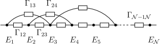
Figure 1: One-dimensional resistor-network model for the one-dimensional variable-range hopping problem described by equation (2). The conductances $\Gamma_{mn}$ are given by (3), $E_{n}$ are random on-site energies.

The master equation (2) is inconvenient in its original form, because its equilibrium distribution $P^{(0)}_{n}=Z^{-1}\exp[-E_{n}/(k_{\rm B}T)]$ is non-uniform. We therefore transform it to an equation evolving towards a uniform equilibrium density, and then describe deviations from this equilibrium in terms of equations analogous to Kirchoff’s laws for a resistor network, with effective conductances $\Gamma_{mn}$ between lattice sites $m$ and $n$. We then expect (following the line of argument employed in Amb72 ) that the diffusion rate is determined by a resistor network (Fig. 1) with ‘conductances’ $\Gamma_{mn}=P^{(0)}_{m}R_{nm}$:

$$\Gamma_{mn}=\epsilon^{|n-m|}{\rm e}^{-{\rm max}(E_{m},E_{n})/(k_{\rm B}T)}\equiv{\rm e}^{-\Delta_{mn}/t}\,.$$ (3)

The last equality defines ‘distances’ $\Delta_{mn}=\alpha t|n-m|+{\rm max}(E_{m},E_{n})$, with $\alpha=-\log\epsilon$, and $t=k_{\rm B}T$.

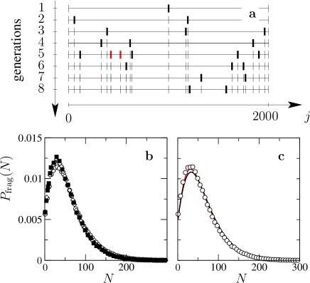
Figure 2: a One realisation of the hierarchical process described ($\alpha=0.1$, $t=0.001$, ${\cal N}=2000$). When segments break they do so mostly by one break (thick black vertical lines). In one instance a segment breaks by two simultaneous breaks (red lines) into three pieces. The process terminates in generation $8$ when all segments are unbreakable. For the particular realisation shown, the percolation approach gives exactly the same segments. b Distribution of hop lengths of the optimal conduction path ($\blacksquare$) determined from a percolation approach. Also shown are approximations employing the hierarchical process, allowing for one ($\circ$) and two ($\Diamond$) breaks per segment. Allowing for more than two simultaneous breaks per interval does not change the distribution significantly. The parameters were $\alpha=0.1$, $t=0.002$, ${\cal N}=5000$. c Stick-breaking approximation for $P_{\rm hop}(N)$ allowing for one break per segment (with the same parameters as in b). We plot equation (11), black line, and on two iterations of (10), red line. Further iterations do not change the red line noticeably. For comparison we show data from the hierarchical scheme allowing one break per segment ($\circ$), as in b.

4. Percolation approach. In the limit as $t\to 0$, ratios between the conductances $\Gamma_{mn}$ become very large. In this limit the fraction of the current in any bond is almost certainly very close to zero (‘inactive bond’), or else very close to unity (‘active bond’). In Amb72 it was pointed out that the resistance of the network is almost surely well approximated by the resistance of the active bond with the highest resistance. This bond can be identified by mapping to a percolation problem: for a given choice of threshold conductance $\Gamma_{0}$, bonds with conductances $\Gamma_{mn}\!<\!\Gamma_{0}$ are removed from the network. Decreasing $\Gamma_{0}$, we test for connectivity of the network. As $\Gamma_{0}$ decreases below the conductance of a ‘critical’ bond, $(n,m)^{\ast}$ (with conductance $\Gamma_{nm}^{\ast}$), we find that the network becomes connected. The conductance of the network is expected to be well approximated by $\Gamma_{mn}^{\ast}$. Now we repeat this procedure for the sub-networks to the left and to the right of the critical bond, determining the critical bonds of the sub-networks. Repeating this procedure results in identifying critical bonds in progressively shorter sections of the network. The process terminates when the critical bond for a sub-network is the one bond that connects its ends directly. In this way the optimal conduction path is found. This approach is accurate when $t\rightarrow 0$, but the search over all possible paths is very time consuming, and not susceptible to statistical analysis. Our objective was to find a way of determining the optimal conduction path by repeated application of simple rules – which can be analysed statistically.

5. Hierarchical model. Our approach consists of breaking down the network by proposing a succession of current-carrying paths with smaller and smaller resistances. At each stage we consider a segment $(m,n)$ of the network, between nodes $m$ and $n$. We ask whether the conductance of the direct connection $\Gamma_{mn}$ is less than that of an indirect path, which goes through an intermediate node $j$. If the resistance $\Gamma^{-1}_{mj}+\Gamma^{-1}_{jn}$ is less than $\Gamma^{-1}_{mn}$, then the network is broken at node $j$, and we consider the sub-networks $(m,j)$ and $(j,n)$. If there is more than one break which lowers the resistance, we choose the one which gives the lowest resistance. If there is no single ‘break’ lowering the resistance, we try inserting two simultaneous breaks, then three, etc. If there is more than one possible way to insert the breaks, the choice giving the lowest resistance is used. If the resistance cannot be reduced below that of the direct connection by considering any sequence of nodes connected in series, then the sub-network is determined to be ‘unbreakable’.

There is no guarantee that the process will produce the optimal conduction path, only that the resistance will decrease with each refinement. As Fig. 2 shows, however, this procedure provides an excellent approximation to the optimal conduction path.

6. Stick-breaking model. The hierarchical method has the advantage that it is easier to analyse than the percolation approach. In the remainder we illustrate this by showing that the simplest hierarchical model (allowing only one break per segment at a time) can be approximated by a ‘stick-breaking model’.

It is found that when an interval can be broken at one point to reduce the resistance, the break point usually corresponds to the site within the interval with the smallest energy $E_{j}$. This observation leads to the following simplified model for the hierarchical process. When considering an interval between sites $n$ and $m$ (with $n>m$), we determine whether the resistance is reduced by inserting a single break. If so, we determine the smallest energy $E_{j}$ with $m<j<n$, and break the interval there. The process of sub-division is continued until all of the intervals are determined to be unbreakable.

In order to model this process we introduce two probabilities. Let $P_{\rm br}(N)$ be the probability that a fragment of length $N$ elements is breakable. If it is breakable, it will break at a position $M$ elements from the end with probability $p(M,N)$. Starting from and infinitely long stick and iterating this process, we end up with a set of unbreakable fragments with a probability $P_{\rm frag}(N)$ for having length $N$. In the following, we discuss how $P_{\rm br}(N)$ and $p(M,N)$ respectively are chosen to make this stick-breaking model correspond to the simplified hierarchical model of variable range hopping. We then discuss how the stick-breaking model is solved. Figure 2c shows that the resulting distribution of fragment lengths, $P_{\rm frag}(N)$, is a good approximation to the distribution of hopping lengths, $P_{\rm hop}(N)$.

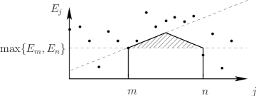
Figure 3: Shows points in $(j,E_{j})$ plane ($j=0,1,2,\ldots$ and $E_{j}$ uniformly distributed on $[0,1]$). The probability that the segment $(m,n)$ is unbreakable (with a single break) is equal to the probability that the ‘roof of the house’ (hashed) of area $A^{\prime}$ is empty. The dashed horizontal line represents $\max\{E_{m},E_{n}\}$, the second dashed line $E_{j}=\max\{E_{m},E_{n}\}+\alpha t\,(j-m)$.

7. Probability for a segment to break. The set of energies can be represented by a set of points in the $j,E_{j}$ plane, which are randomly distributed in energy, with the density of points in the plane being unity.

In the limit of $t\to 0$, the resistance of an indirect path through one intermediate node is approximated by the larger resistance of the two links, so that we write $\Gamma^{-1}_{mj}+\Gamma^{-1}_{jn}\sim\exp[{\rm max}(\Delta_{mj},\Delta_{jn})/t]$. So the probability for a segment $[m,n]$ to be unbreakable is the probability that $\Delta_{nj}>\Delta_{nm}$ and $\Delta_{jm}>\Delta_{nm}$ for any choice of $j$ (with $m<j<n$). These two conditions imply that the regions below two lines in the $(j,E_{j})$ plane are empty, in the interval $[m,n]$. Thus the probability that the interval $[m,n]$ is unbreakable (with a single break) is equal to the probability of finding the ‘house’ in Fig. 3 empty.

The probability of finding a region in the $(j,E_{j})$ plane of area $A$ to be empty of points is $\exp(-A)$. At first sight it seems as if we should take $A$ to be the area of the ‘house’ in figure 3 and the probability that a segment is breakable would be $P_{\rm br}=1-{\rm e}^{-A}$. We do however have some prior knowledge about the energies: because we always break at the minimum energy, the none of the energies $E_{j}$ in the interval $[m,n]$ is less than ${\rm max}(E_{n},E_{m})$. Thus it is the area of the ‘roof’ of the house (hashed in Fig. 3) which is relevant, and the probability for this segment being breakable is therefore

$$P_{\rm br}(n-m)=1-\exp(-A^{\prime})\ ,\ \ \ A^{\prime}=\alpha t(n-m)^{2}/4\,.$$ (4)

Thus the probability for a segment being breakable in our construction is, in fact, solely dependent on its length, and given by (4).

8. Distribution of break points. Next we consider the probability $p(M,N)$ that an interval of length $N$ will break at a position $M$ units from one of its ends. Because the energies $E_{j}$ are independently and identically distributed, we might expect that the position of minimal $E_{j}$ is uniformaly distributed, that is $p(M,N)$ should be independent of $M$. This is incorrect, however, because we are considering the distribution of energies in an interval which is selected to be breakable.

The probability $p(M,N)$ for the position $M$ of minimal $E_{j}$ in an interval of length $N$ is symmetric around the midpoint of the segment. Let $x\in[0,1]$ be a variable measuring distance of the break from the end of the interval, setting $x=2M/(N-1)$ if $M<N/2$ and $x=2(N-M)/(N-1)$ if $N/2<M<N$. We consider the continuous probability density $p(x)$ for $x$, which is related to $p(M,N)$ by:

$$p(M,N)={\frac{1}{N-1}}\left\{\begin{array}[]{ll}p\big{(}{2M\over N\!-\!1}\big{)}&\mbox{if $0<M<N/2$}\\[2.84526pt] p\big{(}{2N-2M\over N\!-\!1}\big{)}&\mbox{$N/2\leq M<N$.}\end{array}\right.$$ (5)

The density $p(x)$ is calculated by geometrical analysis of Fig. 3. We rescale the energy $E_{j}$ to a new variable $y=(N-1)[E_{j}-{\rm max}(E_{n},E_{m})]$ so that the density of points in the $(x,y)$ plane is unity. In these new coordinates the line determining the boundary of the region which must be occupied to ensure breakability is $y=\nu x$ with $\nu=\alpha tN^{2}/2$. Instead of calculating $p(x)$ we compute the complementary probability density $q(x)$, that is the probability density for the position of the minimum energy in an unbreakable segment. The probability density for the location of minima irrespective of breakability is uniform (and by normalisation equal to unity), so that $1=P_{\rm br}p(x)+(1-P_{\rm br})q(x)$, or:

$$p(x)=[{1-\exp(-\nu/2)q(x)}]/[{1-\exp(-\nu/2)}]\,.$$ (6)

It is easier to compute $q(x)$ because the conditional knowledge about unbreakable (at one break) intervals is simpler. These intervals have no points in the $(x,y)$ plane inside the ‘forbidden’ triangle $0<y\!<\!\nu x$, $0\!<\!x\!<\!1$. Thus $q(x)$ is the distribution of $x$ for the point with minimal $y$ from a random, unit density scatter in the ‘allowed’ region $y\!>\!\nu x$, $0\!<\!x\!<\!1$. Let $F(y_{0})$ be the probability that the point with lowest value of $y$ is above $y_{0}$. This satisfies $F(0)=1$ and ${\rm d}F/{\rm d}y=-{\rm d}A/{\rm d}y\,F$ where $A(y)$ is the area of the allowed region below $y$. We have

$$q(x)=\int_{0}^{\infty}\!\!\!\!{\rm d}y\,\bigg{|}\frac{dF}{dy}\bigg{|}\,\chi_{[0,x(y)]}(x)\,\frac{1}{x(y)}$$ (7)

where $\chi_{[a,b]}(x)$ is the characteristic function (equal to unity on the interval $[a,b]$ and zero elsewhere) and $x(y)={\rm d}A/{\rm d}y$ is the width of the allowed region at $y$. Using the differential equation for $F(y)$ we obtain $q(x)=\int_{\nu x}^{\infty}{\rm d}y\ F(y)$. We find $F(y)={\rm e}^{-y^{2}/2\nu}$ for $0<y<\nu$ and $F(y)={\rm e}^{-y+\nu/2}$ for $y>\nu$ and finally obtain:

$$q(x) = {\rm e}^{-{\nu}/{2}}\!+\!\sqrt{{\pi\nu\over{2}}}\biggl{[}{\rm erf}\biggl{(}\sqrt{{\nu\over 2}}\biggr{)}\!-\!{\rm erf}\biggl{(}x\sqrt{\nu\over 2}\biggr{)}\biggr{]}\,.$$ (8)

Eqs. (5-8) show that segments are more likely to break in the centre, as expected. This bias is the stronger the shorter the segments are. For long segments ($\nu\to\infty$) we obtain $p(M,N)\approx 1/(N-1)$. We find that a good approximation to $q(x)$ is

$$q(x)\approx 1+\nu\,(1/2-x)\,.$$ (9)

9. Self-consistent solution of the stick-breaking process. We now determine the probability distribution $P_{\rm frag}(N)$ of the lengths of the unbreakable fragments, by extending a calculation for the distribution of strength of a repeatedly broken random chain, discussed in Wil07 . We start from a very long stick, and after $T$ steps of this process, we have $W_{\rm D}(N,T)$ segments of length $N$ which have been determined to be unbreakable, and $W_{\rm U}(N,T)$ segments of length $N$ which have not yet been tested. Assuming that these numbers are so large that it is sufficient to consider expectation values, we have the recursion $W_{\rm U}(N,T+1)=2\sum_{M=N+1}^{\infty}p(N,M)P_{\rm br}(M)W_{\rm U}(M,T)$ and $W_{\rm D}(N,T+1)=[1-P_{\rm br}(N)]\,W_{\rm U}(N,T)$. Rather than following this iteration for a single stick being broken, we consider a steady state of $W_{\rm U}(N,T)$, with destruction of one additional stick being initiated at each step:

$$W(N)=2\sum_{M=N+1}^{\infty}p(N,M)P_{\rm br}(M)W(M)\,.$$ (10)

The corresponding probability distribution of fragment lengths (or hop lengths) is $P_{\rm frag}(N)=Z^{-1}[1-P_{\rm br}(N)]W(N)$ where $Z$ is a normalisation factor.

When $p(N,M)=1/(M-1)$, equation (10) is solvable. Replacing sums by integrals, we obtain $W_{0}(N)\propto N^{-2}\,{\rm e}^{-{\rm Ei}(\alpha tN^{2}/4)}$, where ${\rm Ei}$ is the exponential integral. When $p(M,N)$ is given by eqs. (5), (6), and (8), we solve (10) by iteration starting with $W_{0}$. Usually a few iterations give an accurate solution. The first iteration gives [using eq. (9) to approximate (8)]

$$P_{\rm frag}(N) \propto {\rm e}^{-\nu/2}[I_{1}(\nu)+I_{2}(\nu)]$$ (11)

$$I_{1}(\nu)\! = \!\int_{\nu}^{4\nu}\frac{{\rm d}\mu}{\mu^{2}}\big{(}{\rm e}^{\mu/2}\!-\!1\!+\!{3\mu\over 2}\!-\!2\sqrt{\mu\nu}\big{)}{\rm e}^{-{\rm Ei}(\mu/2)-\mu/2}$$

$$I_{2}(\nu)\! = \!\int_{4\nu}^{\infty}\frac{{\rm d}\mu}{\mu^{2}}\big{(}{\rm e}^{\mu/2}\!-\!1\!-\!{\mu\over 2}\!+\!2\sqrt{\mu\nu}\big{)}{\rm e}^{-{\rm Ei}(\mu/2)-\mu/2}\,.$$

The distribution $P_{\rm frag}(N)$ given by (11) is shown in Fig. 2c. Results obtained from higher iterations of (10) using (8) are also shown. They converge rapidly and provide a strikingly accurate approximation to $P_{\rm hop}(N)$.

Support from Vetenskapsrådet is gratefully acknowledged.

References

- (1) N. F. Mott, J. Non-Cryst. Solids, 1, 1, (1968).
- (2) V. Ambegoakar, L. S. Langer and B. I. Halperin, Phys. Rev. B, 4, 2612 (1971).
- (3) J. Kurkijärvi, Phys. Rev. B, 8, 622, (1973).
- (4) M. E. Raikh and I. M. Ruzin, Sov. Phys. JETP, 66, 642-7, (1989) [Zh. Eksp. Teor. Fiz., 95, 1113-22, (1989).]
- (5) A. L. Efros and B. I. Shklovskii, J. Phys. C: Solid State Phys. , 8, L49, 1975
- (6) P. A. Lee, Phys. Rev. Lett., 53, 2042, (1984).
- (7) M. Wilkinson and B. Mehlig, J. Stat. Phys., 127, 1279, (2007).