Aspects of power corrections in hadron-hadron collisions

Abstract:

The program of understanding inverse-power law corrections to event shapes and energy flow observables in $e^{+}e^{-}$ annihilation to two jets and DIS (1+1) jets has been a significant success of QCD phenomenology over the last decade. The important extension of this program to similar observables in hadron collisions is not straightforward, being obscured by both conceptual and technical issues. In this paper we shed light on some of these issues by providing an estimate of power corrections to the inter-jet $E_{t}$ flow distribution in hadron collisions using the techniques that were employed in the $e^{+}e^{-}$ annihilation and DIS cases.

1 Introduction

The principle issue that limits the accuracy of theoretical predictions in QCD is the presence of non-perturbative physics responsible for the confinement of quarks and gluons. The success of perturbative QCD, despite a lack of quantitative understanding of the confinement process, is a major achievement that is based on identifying infrared and collinear-safe observables [1] which are as insensitive as possible to non-perturbative effects such as hadronisation. In such instances the role of non-perturbative effects is reduced to the level of corrections to the perturbative estimates which take the form of an inverse-power law in the hard scale $Q$, $1/Q^{p}$, where $p$ depends on the observable. For some observables, such as the total cross-section in $e^{+}e^{-}$ annihilation to jets, where $p=4$, the corrections in question are insignificant and can safely be ignored in comparisons to data. For other observables such as event-shape variables (see ref. [2] for a review) it was noted however that the power corrections scale as $1/Q$ and obscure the perturbative analysis significantly.

Over the past decade, theoretical efforts essentially based on renormalons (see ref. [3] and references therein) have given a clearer picture of the origin and role of power corrections. Within the renormalon model these corrections are shown to be related to a factorial divergence of the perturbative QCD expansion at high orders and the consequent error in truncating what is in fact an asymptotic series [3]. This observation allows one to estimate power corrections from a lowest-order Feynman graph, modified to incorporate the relevant subset of higher-order terms (renormalon bubble insertions).

From a phenomenological viewpoint, perhaps the most widely used formulation of the renormalon model is one that uses a dispersive representation of the running coupling [4], thereby introducing a dispersive variable $m$ that plays the role of a fake gluon mass [5]. This scale is a natural trigger for power corrections arising in the infrared regime for observables that are otherwise dominated by a hard scale $Q$. The most appealing feature of the dispersive approach is the hypothesis of a universal infrared-finite coupling $\alpha_{s}$. The overall size of the power corrections in this approach is related to moments of this universal coupling: $\int_{0}^{\infty}dm^{2}/m^{2}\alpha_{s}(m^{2})(m^{2}/Q^{2})^{p}$. For most event-shape variables (for example) $p=1/2$ [2], and the relevant coupling moment or equivalently the related quantity $\alpha_{0}$ has been extracted from data for different event shapes in both $e^{+}e^{-}$ annihilation and DIS [6, 7]. The values of $\alpha_{0}$ thus obtained have generally confirmed the universality hypothesis to within the expected uncertainties due to missing higher-order corrections [2]. These studies have not only enabled successful studies of several observables, but also lent credence to the notion that the QCD coupling may be a meaningful (finite and universal) concept all the way down to the smallest energy scales, and have thus renewed hope of a better understanding of the confinement domain from first principles of QCD.

The success of renormalon-inspired studies has thus far been limited to observables which involve just two hard partons at Born level such as event shapes in $e^{+}e^{-}\rightarrow$ two jets and DIS ($1+1$) jets. Some of the most interesting QCD observables however do not fall into the above class. Examples include three-jet event shapes in $e^{+}e^{-}$ annihilation and DIS [8, 9, 10, 11], dijet event shapes in hadron collisions [12] and single-jet inclusive cross-sections at hadron colliders [13]. These observables contain more than two hard partons at Born level and additionally pertain to processes that have gluons at Born level where one may question the extension of the dispersive approach, which (strictly speaking) was formulated for observables involving only quarks at the Born level [4]. The program of understanding power corrections has not been put to test in such situations which will be of importance at the LHC, for instance, although some progress is being made on the phenomenological side for three-jet event shapes [11]. In fact for the case of observables involving four hard partons at the Born level there are as yet no theoretical predictions for power corrections.

Applying the renormalon model, in many such cases, reduces (as for $e^{+}e^{-}$ annihilation to jets or DIS event shapes) to an analysis of soft gluon radiation with transverse momenta $k_{t}\sim\Lambda_{\mathrm{QCD}}$, which are associated with a universal infrared-finite coupling. Given the rich structure (colour and geometry-dependence) of soft gluon radiation for processes like dijet production in hadron collisions, it is indeed enticing to see how a perturbative structure may influence predictions for power corrections as predicted by the renormalon model. Signs of perturbatively calculable colour structure in the non-perturbative power-behaved component would strongly suggest that the renormalon-inspired picture of these corrections is an extension of soft gluon radiation, with a modified but universal coupling, thereby conclusively establishing the model.

In this paper we provide a calculation of the power correction to the transverse energy ($E_{t}$) flow away from jets accompanying hard dijet production in hadron collisions. A variant of this observable (the “pedestal height”) was suggested several years ago as a means of separating perturbative bremsstrahlung from the contribution of the soft underlying event in hadron collisions [14]. To date however a satisfactory understanding of the away-from-jet energy flow has proved elusive. In the region of small $E_{t}$ the distribution $d\sigma/dE_{t}$ contains large logarithms of the form $\alpha_{s}^{n}\ln^{n-1}(P_{t}/E_{t})/E_{t}$, where $P_{t}$ is the hard scale (jet transverse momenta) of the problem. These logarithms can only be resummed in the large $N_{c}$ limit [15, 16, 17] which limits the accuracy of perturbative estimates that can be made in this case alongside the lack of any estimates of the NLL contributions. One may also expect power corrections of the form $1/P_{t}$ to the resummed distribution as for the case of event-shape distributions in $e^{+}e^{-}$ annihilation and DIS. Once again there is no estimate for these power corrections and it is this that we aim to provide here. Combining the power corrections we compute with resummed $E_{t}$ flow distributions gives a more complete theoretical account which should facilitate comparisons to experiment.

While at hadron colliders the ever-present soft underlying event may obstruct clean studies of power-behaved corrections arising from the bremsstrahlung component of the $E_{t}$ flow, our calculations here are also easily adapted to the case of rapidity gaps in dijet photoproduction at HERA, and are in principle more readily tested in that environment. Moreover there are theoretical ideas concerning observables such as inclusive jet cross-sections at hadron colliders, where it may be possible to disentangle the underlying event from the non-perturbative physics in the bremsstrahlung component, due to a singular $1/R$ ($R$ being a jet radius parameter) behaviour of the latter [13]. A full estimate of this piece however involves a calculation similar to the one we introduce here and thus the present calculations can be used as a guide in moving towards better estimates of the inclusive jet cross-sections as well. Another related class of observables, to which the techniques we use here are directly applicable, is the important case of event shapes at hadron colliders [12], for which resummed perturbative estimates already exist and identical considerations to those of this paper will be required when dealing with the issue of power corrections. While other problems such as lack of knowledge about next-to-leading logarithms also need to be addressed, the calculation of the power correction is ultimately an important ingredient which, as we stressed above, also serves as a case study for hadron-hadron observables more generally.

This paper is organised as follows. In the following section we define the observable more precisely and review the perturbative result in Mellin space conjugate to $E_{t}$, which involves colour matrices in the resummed anomalous dimensions [18, 19, 20, 21]. We then compute the power correction to each of the matrix elements of the anomalous dimension by considering the appropriate combination of dipoles involved in that matrix element. The calculation of the power correction in each dipole term is performed using the appropriate scale of the running coupling (the invariant transverse momentum of the dipole, $k_{\perp}$ [8, 9, 10, 22, 23, 24]). The final step is to take the inverse Mellin transform of the result including non-perturbative corrections, for which it proves convenient to diagonalise the power-corrected anomalous dimension matrices.We find that the power correction to the $E_{t}$ distribution is not a simple shift of the resummed distribution by a fixed amount proportional to $1/P_{t}$ as is the case for event shapes in $e^{+}e^{-}\rightarrow$ two jets and DIS (to a good approximation).

2 Resummed perturbative result

Here we outline the resummed result for the $E_{t}$ flow distribution accompanying hard dijet production in hadronic collisions, which was originally computed in ref. [25], specialising for simplicity to the case of a slice in rapidity of width $\Delta\eta$, which we take to be centred at $\eta=0$ (the rapidity $\eta$ and transverse energy $E_{t}$ are both defined with respect to the beam direction). We also work, again purely for the sake of convenience, with fixed jet transverse momenta $P_{t}$ and rapidities but can easily generalise to other differential distributions of the hard dijet system. The observable we compute is then the integrated distribution:

$$\Sigma(P_{t},E_{t})=\frac{1}{\sigma_{0}}\int_{0}^{E_{t}}\frac{d\sigma}{dE_{t}^{\prime}}dE_{t}^{\prime},\qquad E_{t}=\sum_{i\in\Omega}E_{t,i},$$ (1)

where $\sigma_{0}$ is the Born cross-section for dijet production (at fixed jet transverse momenta and rapidities) in hadron collisions, $\Omega$ denotes the rapidity slice and $E_{t}$ is obtained by summing over all objects (partons/jets) in the gap.

Since we are examining the accompanying $E_{t}$ flow distribution, we are dealing typically with $E_{t}\ll P_{t}$ and hence there arises the need to resum large logarithms of the form $\alpha_{s}^{n}\ln^{m}(P_{t}/E_{t})$, with $m\leq n$. The resummed prediction for $\Sigma(P_{t},E_{t})$ up to single-logarithmic accuracy (resumming all the terms $\alpha_{s}^{n}\ln^{n}(P_{t}/E_{t})$ in the logarithm of the integrated distribution), can be thought of as comprising two distinct pieces with different dynamical origins: “global” and “non-global” [15, 16].

The first piece (the so-called “global” component) is a result of considering multiple soft emissions, both real and virtual, which are attached just to the primary or Born hard partons. Due to infrared-safety of the observable real and virtual emissions cancel below the scale $E_{t}$, while real emissions above this scale are vetoed. Thus the resummed result for this piece is just the summation of virtual graphs above the scale $E_{t}$, attached to the primary hard partons [18, 19, 20, 21]. In actual fact the factorisation of real emissions and the consequent cancellation with virtual ones takes place in Mellin space conjugate to $E_{t}$. This complication can be ignored for the leading single-logarithmic terms, but to analyse the impact of power corrections on the resummed distribution we need to compute the result in Mellin space and then invert the transform to $E_{t}$ space. To be more precise the perturbative resummed result (considering just the above described global term for now) reads (see for instance ref. [17]):

$$\Sigma(P_{t},E_{t})=\int\frac{d\nu}{2\pi i\nu}e^{\nu E_{t}}\mathcal{R}(\nu),\,$$ (2)

where $\nu$ is the Mellin variable conjugate to $E_{t}$ and the integration contour is taken, in the usual manner, parallel to the imaginary axis and to the right of all singularities of the integrand. We have:

$$\mathcal{R}(\nu)=\mathrm{Tr}\left(\mathbf{H}e^{-\mathbf{\Gamma}^{\dagger}(\nu)}\mathbf{S}e^{-\mathbf{\Gamma}(\nu)}\right)/\Sigma_{0}.$$ (3)

In the above $\mathbf{\Gamma}$ is essentially an “anomalous dimension matrix” and $\mathbf{H}$ and $\mathbf{S}$ are the “hard” and “soft” matrices. The matrix elements $H_{ij}$ represent the product of the Born amplitude in colour channel $i$ and its complex conjugate in colour channel $j$, and the matrix $\mathbf{S}$ represents the normalisation arising from the colour algebra. The squared matrix element for the Born scattering in this notation is just $\Sigma_{0}=\mathrm{Tr}(\mathbf{H}\mathbf{S})$. We shall return to the detailed structure of $\mathbf{\Gamma}$ in the next section but it is important to point out here that all the matrices above depend on the partonic $2\to 2$ sub-process considered, e.g. they differ for say $q\bar{q}\to q\bar{q}$ and $gg\to gg$ sub-processes. Their form also depends on one’s choice of colour basis. For examples the reader is pointed to the original references [18, 19, 20, 21]. We also point out that since we deal exclusively with soft radiation and differential distributions in the jet rapidities and transverse momenta, the parton distribution functions simply factor from the resummed result and cancel against those in the normalisation factor $\sigma_{0}$.

We now turn to the second piece of resummed distribution: the “non-global” contribution. The above result, resumming essentially virtual corrections above the veto scale $E_{t}$ which dress the hard scattering, is not the complete description at single-logarithmic accuracy [15, 16]. An additional “non-global” piece $\mathcal{S}(P_{t},E_{t})$ arises (starting at the two-gluon emission level, $\mathcal{O}(\alpha_{s}^{2})$) and is also single-logarithmic. The dynamical origin of this piece is multiple soft energy-ordered radiation with an arbitrary complex geometry (“hedgehog” configurations of soft gluons, as opposed to emissions strongly ordered in angle). It has thus far been possible to treat this term only in the large $N_{c}$ approximation, which limits the accuracy of perturbative calculations in the present instance.

However it has been pointed out and clarified in a series of papers [27, 28, 29, 30] that the role of the non-global component can be significantly reduced by defining the observable in terms of soft jets rather than individual hadrons in the gap. This can be achieved by running a clustering algorithm on the final states such that all objects are included in jets. The clustering procedure (with a large cluster radius $R=1$) was shown to virtually eliminate the non global component while giving rise to additional global terms [29] that were at most modest corrections to the pure virtual dressing as represented here by eq. (3). Moreover the power corrections associated to the non-global component of the result would start at a higher-order in $\alpha_{s}$ (albeit potentially accompanied by logarithms of $P_{t}/E_{t}$) which we ignore. This was also the procedure employed for the case of non-global DIS event shapes [2], where power corrections were computed in the exponentiated single-gluon piece of the resummed distribution, which was a phenomenological success. For all these reasons we shall choose to concentrate for the rest of this paper on the global component (eq. (3)), ignoring the non-global component.

In the following section we explicate the structure of $\mathbf{\Gamma}$ in terms of the various hard colour dipoles from which one considers soft gluons to be emitted according to the usual antenna pattern. Non-perturbative power corrections are then computed on a dipole-by-dipole basis, adapting the procedure for a $q\bar{q}$ dipole developed for the case of $e^{+}e^{-}$ annihilation to two jets. Having obtained the power corrections to $\mathbf{\Gamma}(\nu)$ we then invert the Mellin transform to examine the result for the $E_{t}$ distribution.

3 The anomalous dimension and power corrections

We first write down the structure of the resummed anomalous dimension matrix $\mathbf{\Gamma}(\nu)$ and then note that it contains an integral over the running coupling which is formally divergent. Making the ansatz of a universal infrared-finite coupling cures this divergence and introduces calculable power corrections to the perturbative anomalous dimensions. In what follows and for the rest of this paper we specialise to the case of the sub-process $q\bar{q}\to q\bar{q}$ since identical considerations are involved for all other sub-processes. Full results combining all sub-processes will be made available in forthcoming work.

For the sub-process $q\left(p_{1},r_{1}\right)+\bar{q}\left(p_{2},r_{2}\right)\to q\left(p_{3},r_{3}\right)+\bar{q}\left(p_{4},r_{4}\right)$, where $p_{i}$ and $r_{i}$ are respectively four-momenta and colour indices, we can choose to work in the $t$-channel singlet-octet colour basis:

$$c_{1}=\delta_{r_{1}r_{3}}\delta_{r_{2}r_{4}},\qquad c_{2}=\frac{1}{2}\left(\delta_{r_{3}r_{4}}\delta_{r_{1}r_{2}}-\frac{1}{N_{c}}\delta_{r_{1}r_{3}}\delta_{r_{2}r_{4}}\right).$$ (4)

For this basis we have:

$$\mathbf{S}=\left(\begin{array}[]{ccc}N_{c}^{2}&0\\ 0&\frac{N_{c}^{2}-1}{4}\end{array}\right),$$ (5)

and the anomalous dimension matrix $\mathbf{\Gamma}$ is:

$$\mathbf{\Gamma}=\left(\begin{array}[]{ccc}C_{F}T&\frac{C_{F}}{2N_{c}}(S-U)\\ S-U&C_{F}S-\frac{1}{2N_{c}}(T-2U+S)\end{array}\right).$$ (6)

In the above $S$, $T$ and $U$ are combinations of dipole contributions with each contribution given by the corresponding dipole antenna. Thus one has:

$$S =\tilde{w}_{12}+\tilde{w}_{34},$$ (7)

$$T =\tilde{w}_{13}+\tilde{w}_{24},$$ (8)

$$U =\tilde{w}_{23}+\tilde{w}_{14},$$ (9)

where each dipole contribution $\tilde{w}_{ij}$ reads:

$$\tilde{w}_{ij}=\int\frac{d^{3}\vec{k}}{2\omega(2\pi)^{3}}g_{s}^{2}\frac{\left(p_{i}.p_{j}\right)}{\left(p_{i}.k\right)\left(p_{j}.k\right)}u(k_{t},\nu).$$ (10)

In the above result we have integrated the soft gluon emission probability, given by the dipole antenna pattern, over the gluon phase-space (with $\vec{k}$ and $\omega$ being respectively the three-momentum and energy of the gluon, as usual) with a “source” function $u(k_{t},\nu)$ and $g_{s}^{2}=4\pi\alpha_{s}$. The source is a result of factorising the real soft emission phase-space in Mellin space (see for instance ref. [17]) and accounting additionally for virtual corrections. It reads:

$$u(k_{t},\nu)=\left(1-e^{-\nu k_{t}}\right),$$ (11)

if the emission is in $\Omega$ and zero elsewhere. The source thus represents the impact of real-virtual contributions which completely cancel, to our accuracy, for emissions outside $\Omega$. Now introducing the variables $\eta$ and $\phi$, respectively the rapidity and azimuth of the emission with respect to the beam direction, one can write:

$$\tilde{w}_{ij}=\int\frac{dk_{t}}{k_{t}}\frac{\alpha_{s}(k_{\perp,i,j}^{2})}{2\pi}d\eta\frac{d\phi}{2\pi}\left(1-e^{-\nu k_{t}}\right)f_{ij}(\eta,\phi),$$ (12)

with $f_{ij}(\eta,\phi)$ being the functional dependence on rapidity and azimuth that arises from the dipole antenna patterns and which we shall use below (see appendix). We note that, to our accuracy, the correct argument of the running coupling for emission from a dipole ([8, 9, 10, 22, 23, 24]) is $k_{\perp,ij}^{2}=2(p_{i}.k)(p_{j}.k)/(p_{i}.p_{j})$, which is the transverse momentum of the gluon $k$ with respect to the dipole axis in the dipole rest frame. This must be distinguished from $k_{t}$, the transverse momentum of the gluon with respect to the beam direction, which is the quantity that directly enters the observable definition. In fact we have, in terms of the functions $f_{ij}$ introduced above, $k_{\perp,ij}=k_{t}\sqrt{2/f_{ij}}$.

3.1 Power corrections dipole-by-dipole

Now we proceed to an extraction of the leading power-behaved contribution. In order to do this we first note that the integral over $k_{t}$ in eq. (12), which can be rewritten as one over the related variable $k_{\perp}$, is divergent if one uses the usual perturbative definition of $\alpha_{s}$, due to the divergence of the perturbative running coupling at $k_{\perp}=\Lambda_{\mathrm{QCD}}$. In order to isolate and cure this pathological behaviour we assume an infrared-finite coupling ($\alpha_{s}$) and change variable of integration from $k_{t}$ to $k_{\perp}$ in eq. (12). We then follow the method of ref. [31] to write $\alpha_{s}(k_{\perp}^{2})=\alpha_{s,\mathrm{PT}}(k_{\perp}^{2})+\delta\alpha_{s,\mathrm{NP}}(k_{\perp}^{2})$, where PT and NP stand for perturbative and non-perturbative respectively. In doing so we have assumed that the actual coupling $\alpha_{s}$ is in fact finite even at arbitrarily small $k_{\perp}$, and can be split into the usual perturbative component $\alpha_{s,\mathrm{PT}}$ and a modification $\delta\alpha_{s,\mathrm{NP}}$ which is due to non-perturbative effects. Both the perturbative and non-perturbative components separately diverge, but the divergences cancel in their sum due to the assumed finiteness of the physical coupling $\alpha_{s}$. Moreover, since we do not wish to modify the perturbative results at large scales, the non-perturbative physics as represented by the modification $\delta\alpha_{s,\mathrm{NP}}$ must vanish above some infrared “matching” scale $\mu_{I}$. Effectively the addition of the $\delta\alpha_{s,\mathrm{NP}}$ term represents removal of the badly-behaved perturbative contribution below $\mu_{I}$ and its replacement with the well-behaved integral over the infrared-finite physical coupling $\alpha_{s}$.

Thus for the observable itself one has from dipole ($ij$):

$$\int_{k\in\Omega}d\eta\frac{d\phi}{2\pi}\frac{dk_{\perp,i,j}}{k_{\perp,i,j}}\frac{\alpha_{s,\mathrm{PT}}(k_{\perp,i,j}^{2})}{2\pi}\left(1-e^{-\nu k_{t}}\right)f_{ij}(\eta,\phi)+\\ +\int_{k\in\Omega}d\eta\frac{d\phi}{2\pi}\frac{dk_{\perp,i,j}}{k_{\perp,i,j}}\frac{\delta\alpha_{s,\mathrm{NP}}(k_{\perp,i,j}^{2})}{2\pi}\left(1-e^{-\nu k_{t}}\right)f_{ij}(\eta,\phi).$$ (13)

The integral involving the perturbative coupling represents the usual perturbative contribution from dipole ($ij$). The leading logarithmic perturbative contribution arises from the region where one can make the approximation:

$$\left(1-e^{-\nu k_{t}}\right)\approx\theta\left(k_{t}-\frac{1}{\nu}\right).$$ (14)

The perturbative results are reported at length in ref. [25]. In what follows we shall consider in more detail the non-perturbative contribution from the integral involving $\delta\alpha_{s,\mathrm{NP}}$.

In order to evaluate the non-perturbative contribution we first consider that the leading such term arises from the region $\mu_{I}\ll 1/\nu$, which translates to a requirement on $E_{t}$ to be above a few GeV. In this region one can expand the exponential in an exactly analogous way as for event-shape distributions [31]. The leading term is given by the first term in the expansion: $1-\exp(-\nu k_{t})\approx\nu k_{t}$, and this corresponds to a linear $1/P_{t}$ power correction. We ignore quadratic and higher power corrections that would scale as $1/P_{t}^{2}$ and beyond, once again following the case of event-shape variables. We also note that in the shape function approach [32, 33, 34], where one may study non-perturbative effects even into the region $E_{t}\sim\Lambda_{\mathrm{QCD}}$, higher powers of $\nu$ need also to be retained. Working with just the leading term gives us the non-perturbative correction from the ($ij$) dipole which can then be written as:

$$\tilde{w}_{ij}=\tilde{w}_{ij}^{\mathrm{PT}}+\nu{\mathcal{P}}C_{ij}.$$ (15)

Here the non-perturbative quantity ${\mathcal{P}}$ is the first moment of the coupling modification $\delta\alpha_{s,\mathrm{NP}}$:

$$\mathcal{P}=\int_{0}^{\mu_{I}}\frac{dk_{\perp}}{k_{\perp}}k_{\perp}\frac{\delta\alpha_{s,\mathrm{NP}}(k_{\perp}^{2})}{2\pi},$$ (16)

which also enters $1/Q$ ($Q$ being the hard scale) power corrections to event shapes and can be related to the parameter $\alpha_{0}$, extracted from fits to event shape data, as:

$$\mathcal{P}=\frac{\mu_{I}}{2\pi}\left(\alpha_{0}(\mu_{I})-\alpha_{s}(P_{t}^{2})-\frac{\beta_{0}}{2\pi}\left(\ln\frac{P_{t}}{\mu_{I}}+\frac{K}{\beta_{0}}+1\right)\alpha_{s}^{2}(P_{t}^{2})+\mathcal{O}(\alpha_{s}^{3})\right),$$ (17)

where $\alpha_{0}(\mu_{I})=1/\mu_{I}\int_{0}^{\mu_{I}}dk_{\perp}\,\alpha_{s}(k_{\perp}^{2})$, $\beta_{0}$ is the first coefficient of the QCD beta function and:

$$K=C_{A}\left(\frac{67}{18}-\frac{\pi^{2}}{6}\right)-\frac{5}{9}n_{f}.$$ (18)

The coefficients $C_{ij}$ represent the integral over directions:

$$C_{ij}=\int_{k\in\Omega}d\eta\frac{d\phi}{2\pi}\frac{1}{\sqrt{2}}f_{ij}^{3/2},$$ (19)

where $f_{ij}$ arises from the dipole antenna pattern as indicated in eq. $\eqref{eq:dip}$, and a further factor proportional to $\sqrt{f_{ij}}$ comes from rewriting $k_{t}$ in terms of $k_{\perp}$ as we stated before. The explicit form of the $f_{ij}$ functions is reported in the appendix. Performing the integrals over $\eta$ and $\phi$ in eq. (19) yields the coefficients $C_{ij}$ that correspond to the non-perturbative contribution to $\tilde{w}_{ij}$ in eq. (15), which we do not explicitly display for economy of presentation.

Having computed the power corrections proportional to $\nu$ for each dipole, we can include these corrections to the anomalous dimension matrix in eq. (6), which can then be written as:

$$\mathbf{\Gamma}=\tau(\nu)\mathbf{\Gamma}_{\mathrm{PT}}+\nu\mathcal{P}\mathbf{\Gamma}_{\mathrm{NP}},$$ (20)

where the non-perturbative contribution $\mathbf{\Gamma}_{\mathrm{NP}}$ is built up by combining the dipole contributions $C_{ij}$ as in the perturbative case. In the case of the perturbative term $\mathbf{\Gamma}_{\mathrm{PT}}$ we explicitly extracted the integral over the transverse momentum of the coupling:

$$\tau(\nu)=\int_{1/\nu}^{P_{t}}\frac{dk_{t}}{k_{t}}\frac{\alpha_{s,\mathrm{PT}}(k_{t}^{2})}{2\pi},$$ (21)

which arises by making the substitution (14) in the first term of (13). Then the matrix $\mathbf{\Gamma}_{\mathrm{PT}}$ is the usual perturbative anomalous dimension containing integrals over gluon directions inside the region $\Omega$. In the following section we shall consider the evaluation of the inverse Mellin transform to take our results from $\nu$ space to $E_{t}$ space.

4 Power corrections in the $E_{t}$ cross-section

After accommodating the leading power corrections (those expected to give rise to $1/P_{t}$ effects) eq. (2) assumes the explicit form:

$$\Sigma(P_{t},E_{t})=\int\frac{d\nu}{2\pi i\nu}e^{\nu E_{t}}\times\\ \times\mathrm{Tr}\left[\mathbf{H}\exp\left(-\tau\mathbf{\Gamma}_{\mathrm{PT}}^{{\dagger}}-\nu\mathcal{P}\mathbf{\Gamma}_{\mathrm{NP}}^{{\dagger}}\right)\mathbf{S}\exp\left(-\tau\mathbf{\Gamma}_{\mathrm{PT}}-\nu\mathcal{P}\mathbf{\Gamma}_{\mathrm{NP}}\right)\right]/\Sigma_{0}.$$ (22)

In order to invert the Mellin transform (perform the $\nu$ integral above) it is simplest to diagonalise the matrix $\tau\mathbf{\Gamma}_{\mathrm{PT}}+\nu\mathcal{P}\mathbf{\Gamma}_{\mathrm{NP}}$. In the basis in which the matrix $\mathbf{\Gamma}$ is diagonal the matrices $\mathbf{H}$ and $\mathbf{S}$ become $\widetilde{\mathbf{H}}=\mathbf{R}^{-1}\mathbf{H}\mathbf{R}^{-1{\dagger}}$ and $\widetilde{\mathbf{S}}=\mathbf{R}^{{\dagger}}\mathbf{S}\mathbf{R}$, where $\mathbf{R}$ is a matrix which contains the eigenvectors of $\mathbf{\Gamma}$ as column entries (see also [35]). After diagonalisation we can write the result for $\Sigma(P_{t},E_{t})$ in terms of components as:

$$\Sigma(P_{t},E_{t})=\int\frac{d\nu}{2\pi i\nu}e^{\nu E_{t}}e^{-\lambda_{i}}\delta_{ij}\widetilde{H}_{jk}e^{-\lambda^{*}_{k}}\delta_{kl}\widetilde{S}_{li}/\Sigma_{0},$$ (23)

where $\lambda_{i}$ are the eigenvalues of the matrix $\mathbf{\Gamma}$. For the case of the $q\bar{q}\to q\bar{q}$ sub-process, which we use as an example, $\mathbf{\Gamma}$, $\widetilde{\mathbf{H}}$ and $\widetilde{\mathbf{S}}$ are $2\times 2$ matrices and the above result can be written explicitly in terms of the elements of the various matrices as:

$$\Sigma(P_{t},E_{t})=\int\frac{d\nu}{2\pi i\nu}e^{\nu E_{t}}\frac{1}{\Sigma_{0}}\times\\ \times\left(\widetilde{H}_{11}\widetilde{S}_{11}e^{-(\lambda_{1}+\lambda_{1}^{*})}+\widetilde{H}_{12}\widetilde{S}_{21}e^{-(\lambda_{1}+\lambda_{2}^{*})}+\widetilde{H}_{21}\widetilde{S}_{12}e^{-(\lambda_{1}^{*}+\lambda_{2})}+\widetilde{H}_{22}\widetilde{S}_{22}e^{-(\lambda_{2}+\lambda_{2}^{*})}\right),$$ (24)

where the above result contains both perturbative and non-perturbative contributions. To separate these we note that the eigenvalues can be expanded so as to retain only the first-order in $\nu$ correction to the perturbative value, which depends logarithmically on $\nu$:

$$\lambda_{i}=\tau(\nu)\lambda_{i}^{\mathrm{PT}}+\nu\mathcal{P}\lambda_{i}^{\mathrm{NP}}+\mathcal{O}(\nu^{2}).$$ (25)

We emphasise here that while $\lambda^{\mathrm{PT}}_{i}$ are simply the eigenvalues of $\mathbf{\Gamma}_{\mathrm{PT}}$, $\lambda^{\mathrm{NP}}_{i}$ are not the eigenvalues of $\mathbf{\Gamma}_{\mathrm{NP}}$. Instead they are coefficients of the $\mathcal{O}(\nu)$ component of the expansion of the eigenvalues of $\tau\mathbf{\Gamma}_{\mathrm{PT}}+\nu\mathcal{P}\mathbf{\Gamma}_{\mathrm{NP}}$ and they depend on the components of both $\mathbf{\Gamma}_{\mathrm{NP}}$ and $\mathbf{\Gamma}_{\mathrm{PT}}$.

The matrices $\widetilde{\mathbf{H}}$ and $\widetilde{\mathbf{S}}$ also differ from their pure perturbative forms by corrections which depend on $\nu$. Let us introduce the notation $D_{ij}=\widetilde{H}_{ij}\widetilde{S}_{ji}$ (summation not implied). We expand the elements $D_{ij}$ to first order in $\nu$ and write the result as:

$$\Sigma(P_{t},E_{t})=\sum_{i,j}\int\frac{d\nu}{2\pi i\nu}e^{\nu\left(E_{t}-\mathcal{P}\left[\lambda_{i}^{\mathrm{NP}}+\lambda_{j}^{*\mathrm{NP}}\right]\right)}\left(D_{ij}^{\mathrm{PT}}+\frac{\nu}{\tau(\nu)}\mathcal{P}D_{ij}^{\mathrm{NP}}\right)e^{-\tau(\nu)(\lambda_{i}^{\mathrm{PT}}+\lambda_{j}^{*\mathrm{PT}})}/\Sigma_{0},$$ (26)

where the sum runs over the components of the matrix $D_{ij}$ and we ignored $\mathcal{O}(\nu^{2})$ terms in the expansion of $D_{ij}(\nu)$, as they would contribute to corrections that scale as $1/E_{t}^{2}$, which are beyond our control with the present method. We shall see that the terms we ignore are expected to be numerically of no significance.

We first write down the pure perturbative result $\Sigma^{\mathrm{PT}}(P_{t},E_{t})$ obtained by ignoring all non-perturbative (NP) components. To perform the $\nu$ integral we use the standard method of expanding $\tau(\nu)$ about the saddle point at $\nu=1/E_{t}$,

$$\tau(\nu)=\tau(1/E_{t})+\ln(\nu P_{t})\left(\frac{\partial\,\tau(\nu)}{\partial\ln(\nu P_{t})}\right)_{\nu=1/E_{t}}+\cdots.$$ (27)

Performing the integral over $\nu$ and noting that the logarithmic derivatives of $\tau(\nu)$ are related to subleading terms of relative order $\alpha_{s}$ to the leading single logarithms, we arrive at the leading-logarithmic resummed result:

$$\Sigma^{\mathrm{PT}}(P_{t},E_{t})\approx\sum_{i,j}D_{ij}^{\mathrm{PT}}e^{-\left(\lambda_{i}^{\mathrm{PT}}+\lambda_{j}^{*\mathrm{PT}}\right)\tau(E_{t})}/\Sigma_{0},$$ (28)

where the effect of the $\nu$ integration amounts to merely replacing $\nu$ by $1/E_{t}$. Now redoing the $\nu$ integral including the non-perturbative correction to the eigenvalues (still ignoring the NP corrections to $D_{ij}$) we find by examining eq. (26) that the impact of the non-perturbative term amounts simply to a shift of the perturbative result in each of the terms in the sum in eq. (28):

$$E_{t}\rightarrow E_{t}-\mathcal{P}\left(\lambda_{i}^{\mathrm{NP}}+\lambda_{j}^{*\mathrm{NP}}\right).$$ (29)

Looking at the distribution in $E_{t}$, with $E_{t}$ being measured in units of the hard scale $P_{t}$, amounts to a $1/P_{t}$ non-perturbative shift in each term in the sum above, as is the case for two-jet event-shape variables [33, 31]. However in contrast to the case of event shapes it should be clear that the overall impact of the power correction is not simply a shift of the perturbative distribution by a fixed amount since each term in the sum on the right hand side of eq. (28) receives its own characteristic shift depending on the sum of the eigenvalues $\lambda_{i}^{\mathrm{NP}}+\lambda_{j}^{*\mathrm{NP}}$ entering the term in question.

We have still not accounted for the non-perturbative contribution to the colour basis as contained in the $D_{ij}^{\mathrm{NP}}$ terms. To evaluate these one performs the contour integral in question which yields a power correction of the form $\mathcal{P}/E_{t}$, which is related to the fact that these pieces are proportional to $\nu$. Computing the full result for this piece using precisely the same expansion about $\nu=1/E_{t}$ as before and discarding perturbative subleading terms beyond single-logarithmic accuracy, we arrive at our final result for $\Sigma(P_{t},E_{t})$:

$$\Sigma(P_{t},E_{t})=\sum_{i,j}e^{-\Delta_{ij}^{\mathrm{PT}}\tau\left(E_{t}-\Delta_{ij}^{\mathrm{NP}}\right)}\left[D_{ij}^{\mathrm{PT}}+D_{ij}^{\mathrm{NP}}\frac{\mathcal{P}}{E_{t}}\frac{1}{\tau(E_{t})}G_{ij}\left(\alpha_{s},\frac{P_{t}}{E_{t}}\right)\right]/\Sigma_{0},$$ (30)

where $\Delta_{ij}^{\mathrm{NP}}=\mathcal{P}(\lambda_{i}^{\mathrm{NP}}+\lambda_{j}^{*\mathrm{NP}})$ and $\Delta_{ij}^{\mathrm{PT}}=\lambda_{i}^{\mathrm{PT}}+\lambda_{j}^{*\mathrm{PT}}$, and the function $G_{ij}$ is approximately a constant of order $\alpha_{s}(P_{t})$, varying very slowly with $E_{t}$ over the range of $E_{t}$ we consider here. It is a function of the logarithmic derivative of the single-log resummed perturbative result and hence scales as $\alpha_{s}$,

$$G_{ij}\equiv\frac{\partial}{\partial\ln(P_{t}/E_{t})}\left(\Delta_{ij}^{\mathrm{PT}}\tau(E_{t})+\ln(\tau\left(E_{t}\right)\right)\approx\alpha_{s}(P_{t}).$$ (31)

We also note the presence of $1/\tau(E_{t})$ accompanying the $1/E_{t}$ dependence above, which is a reflection of the fact that the correction terms (involving $D_{ij}^{\mathrm{NP}}$) go as $\nu/\tau$.

5 Results and conclusions

In this section, for completeness, we illustrate the impact of non-perturbative power corrections on the energy flow distribution we discussed above.

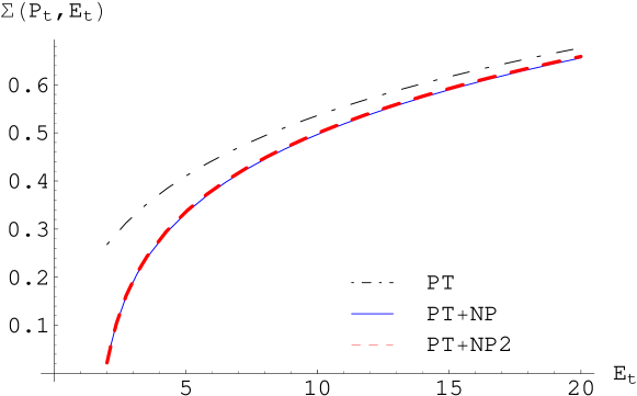
Figure 1: Power corrections to the energy flow distribution. PT stands for the pure perturbative result $\Sigma^{\mathrm{PT}}(P_{t},E_{t})$ as presented in eq. (28), PT+NP stands for the result including the non-perturbative correction and ignoring the terms $D_{ij}^{\mathrm{NP}}$, while PT+NP2 stands for the result presented in eq. (30).

In fig. 1 we show the result for $\Sigma(P_{t},E_{t})$. We present the pure perturbative result (eq. (28)), the result including non-perturbative corrections without the $D_{ij}^{\mathrm{NP}}$ component (PT+NP) and the result presented in eq. (30) (PT+NP2).

The results above were obtained for the illustrative value of $p_{t}=80$ GeV and fixing jet rapidities at -2.5 and 0.9 units respectively. We have performed the integration over the functions $f_{ij}^{3/2}$ for the non-perturbative component (given in eq. (19)) numerically. We also assumed that the rapidity gap has width $\Delta\eta=1$.

We notice that the effect of the term $D_{ij}^{\mathrm{NP}}$ is in fact very small and can be safely ignored which is as an indication that neglected higher orders in the expansion of $D_{ij}$ are even more suppressed. We obtain as expected only a few percent correction to the resummed perturbative result even at fairly low $E_{t}$, which given the remaining theoretical uncertainties (notably having only the large $N_{c}$ control over even leading logarithms) is not significant in itself. However our main motivation as stressed in the introduction, has not been the immediate phenomenology of the $E_{t}$ flow observable, but rather a study of how power corrections may be included in resummed predictions for general observables in hadronic dijet production, since the soft function we treated here generically appears in resummation of global hadronic dijet observables.

In conclusion, we have carried out for the first time a calculation of power corrections to transverse energy flow associated with dijet production in hadron-hadron collisions. We illustrated the computation for the energy flow distribution using the process $q\bar{q}\rightarrow q\bar{q}$. The generalisation to other channels is straightforward and only requires the numerical computation of the diagonalised anomalous dimensions and the corresponding hard and soft matrices. We found that the result does not correspond to the usual shift found in studies of two-jet event shapes and energy flows. The reason for this is the non-trivial colour algebra involved in the case of hadron collisions. The techniques we used here should enable better estimates of power corrections for observables which have a similar nature to the one we introduced here, such as the global inclusive jet cross-section we mentioned earlier.

We re-emphasise that the simple calculation of this paper is just a first step in the full quantitative estimate of power corrections, pending the inclusion of two-loop effects. In the simpler cases of $e^{+}e^{-}\to 2$ jets and DIS (1+1) jet processes, two-loop effects merely rescaled the simple one gluon calculation by a universal (Milan) factor [36, 37, 38, 39], which arises when considering a two-loop analysis for the argument of the coupling. We shall leave the inclusion of such effects to forthcoming work.

Appendix A The functions $f_{ij}$

We present here expressions for the functions $f_{ij}$. We define $\eta_{3}$ and $\eta_{4}$ to be the rapidities of the outgoing hard legs. We specify the kinematics of the particles as follows:

$$p_{1} = x_{1}\sqrt{s}/2\left(1,0,0,-1\right),$$ (32)

$$p_{2} = x_{2}\sqrt{s}/2\left(1,0,0,1\right),$$ (33)

$$p_{3} = P_{t}\left(\cosh\eta_{3},1,0,\sinh\eta_{3}\right),$$ (34)

$$p_{4} = P_{t}\left(\cosh\eta_{4},-1,0,\sinh\eta_{4}\right),$$ (35)

$$k = k_{t}\left(\cosh\eta,\cos\phi,\sin\phi,\sinh\eta\right),$$ (36)

where $s$ is the hadronic centre-of-mass energy squared, related to $\hat{s}$ (the partonic centre-of-mass energy squared) by $\hat{s}=x_{1}x_{2}s$, with $x_{1}$ and $x_{2}$ being the momentum fractions of the incoming protons, carried by the incoming partons “1” and “2” respectively.

The functions $f_{ij}(\eta,\phi)=k_{t}^{2}\,p_{i}.p_{j}/(p_{i}.k\,p_{j}.k)$, are given by:

$$f_{12} = 2,$$ (37)

$$f_{13} = \frac{e^{\eta_{3}-\eta}}{\cosh(\eta_{3}-\eta)-\cos\phi},$$ (38)

$$f_{14} = \frac{e^{\eta_{4}-\eta}}{\cosh(\eta_{4}-\eta)+\cos\phi},$$ (39)

$$f_{23} = \frac{e^{-\eta_{3}+\eta}}{\cosh(\eta_{3}-\eta)-\cos\phi},$$ (40)

$$f_{24} = \frac{e^{-\eta_{4}+\eta}}{\cosh(\eta_{4}-\eta)+\cos\phi},$$ (41)

$$f_{34} = \frac{\cosh(\eta_{3}-\eta_{4})+1}{(\cosh(\eta_{3}-\eta)-\cos\phi)(\cosh(\eta_{4}-\eta)+\cos\phi)}.$$ (42)

References

- [1] G. Sterman and S. Weinberg, Jets From Quantum Chromodynamics, Phys. Rev. Lett. 39 (1977) 1436.
- [2] M. Dasgupta and G. P. Salam, Event shapes in annihilation and deep inelastic scattering, J. Phys. G 30 (2004) R143 [hep-ph/0312283].
- [3] M. Beneke, Renormalons, Phys. Rept. 317 (1999) 1 [hep-ph/9807443].
- [4] Y. L. Dokshitzer, G. Marchesini and B. R. Webber, Dispersive Approach to Power-Behaved Contributions in QCD Hard Processes, Nucl. Phys. B 469 (1996) 93 [hep-ph/9512336].
- [5] P. Ball, M. Beneke and V. M. Braun, Resummation of ( corrections in QCD: Techniques and applications to the hadronic width and the heavy quark pole mass, Nucl. Phys. B 452 (1995) 563 [hep-ph/9502300].
- [6] S. Kluth, Power corrections in electron positron annihilation: Experimental review, In the Proceedings of FRIF workshop on first principles non-perturbative QCD of hadron jets, LPTHE, Paris, France, 12-14 Jan 2006, pp R002 [hep-ex/0606046].
- [7] T. Kluge, Review of power corrections in DIS, In the Proceedings of FRIF workshop on first principles non-perturbative QCD of hadron jets, LPTHE, Paris, France, 12-14 Jan 2006, pp R003 [hep-ex/0606053].
- [8] A. Banfi, Y. L. Dokshitzer, G. Marchesini and G. Zanderighi, Near-to-planar 3-jet events in and beyond QCD perturbation theory, Phys. Lett. B 508 (2001) 269 [hep-ph/0010267].
- [9] A. Banfi, Y. L. Dokshitzer, G. Marchesini and G. Zanderighi, Non-perturbative QCD analysis of near-to-planar three-jet events, J. High Energy Phys. 03 (2001) 007 [hep-ph/0101205].
- [10] A. Banfi, Y. L. Dokshitzer, G. Marchesini and G. Zanderighi, QCD analysis of D-parameter in near-to-planar three-jet events, J. High Energy Phys. 05 (2001) 040 [hep-ph/0104162].
- [11] A. Banfi, Three-jet event-shapes: first NLO+NLL+ results, To appear in the proceedings of International Workshop on Deep-Inelastic Scattering and Related Subjects (DIS 2007), Munich, Germany, 16-20 Apr 2007 [\arXivid0706.2722].
- [12] A. Banfi, G. P. Salam and G. Zanderighi, Resummed event shapes at hadron hadron colliders, J. High Energy Phys. 08 (2004) 062 [hep-ph/0407287].
- [13] M. Cacciari, M. Dasgupta, L. Magnea and G. Salam, Power corrections for jets at hadron colliders, To appear in the proceedings of International Workshop on Deep-Inelastic Scattering and Related Subjects (DIS 2007), Munich, Germany, 16-20 Apr 2007 [\arXivid0706.3157].
- [14] G. Marchesini and B. R. Webber, Associated transverse energy in hadronic jet production, Phys. Rev. D 38 (1988) 3419.
- [15] M. Dasgupta and G. P. Salam, Resummation of non-global QCD observables, Phys. Lett. B 512 (2001) 323 [hep-ph/0104277].
- [16] M. Dasgupta and G. P. Salam, Accounting for coherence in interjet flow: A case study, J. High Energy Phys. 03 (2002) 017 [hep-ph/0203009].
- [17] A. Banfi, G. Marchesini and G. Smye, Away-from-jet energy flow, J. High Energy Phys. 08 (2002) 006 [hep-ph/0206076].
- [18] J. Botts and G. Sterman, Hard Elastic Scattering in QCD: Leading Behavior, Nucl. Phys. B 325 (1989) 62.
- [19] N. Kidonakis and G. Sterman, Subleading logarithms in QCD hard scattering, Phys. Lett. B 387 (1996) 867.
- [20] N. Kidonakis and G. Sterman, Resummation for QCD hard scattering, Nucl. Phys. B 505 (1997) 321 [hep-ph/9705234].
- [21] N. Kidonakis, G. Oderda and G. Sterman, Evolution of color exchange in QCD hard scattering, Nucl. Phys. B 531 (1998) 365 [hep-ph/9803241].
- [22] A. Banfi, G. Marchesini, Y. L. Dokshitzer and G. Zanderighi, QCD analysis of near-to-planar 3-jet events, J. High Energy Phys. 07 (2000) 002 [hep-ph/0004027]
- [23] S. Catani and M. Grazzini, Infrared factorization of tree level QCD amplitudes at the next-to-next-to-leading order and beyond, Nucl. Phys. B 570 (2000) 287 [hep-ph/9908523].
- [24] S. Mert Aybat, L. J. Dixon and G. Sterman, The two-loop soft anomalous dimension matrix and resummation at next-to-next-to leading pole, Phys. Rev. D 74 (2006) 074004 [hep-ph/0607309].
- [25] C. F. Berger, T. Kucs and G. Sterman, Energy flow in interjet radiation, Phys. Rev. D 65 (2002) 094031 [hep-ph/0110004].
- [26] J. R. Forshaw, A. Kyrieleis and M. H. Seymour, Super-leading logarithms in non-global observables in QCD?, J. High Energy Phys. 08 (2006) 059 [hep-ph/0604094].
- [27] R. B. Appleby and M. H. Seymour, Non-global logarithms in inter-jet energy flow with clustering requirement, J. High Energy Phys. 12 (2002) 063 [hep-ph/0211426].
- [28] A. Banfi and M. Dasgupta, Problems in resumming interjet energy flows with clustering, Phys. Lett. B 628 (2005) 49 [hep-ph/0508159].
- [29] Y. Delenda, R. Appleby, A. Banfi and M. Dasgupta, On QCD resummation with clustering, J. High Energy Phys. 12 (2006) 044 [hep-ph/0610242].
- [30] R. B. Appleby and M. H. Seymour, The resummation of inter-jet energy flow for gaps-between-jets processes at HERA, J. High Energy Phys. 09 (2003) 056 [hep-ph/0308086].
- [31] Y. L. Dokshitzer and B. R. Webber, Power corrections to event shape distributions, Phys. Lett. B 404 (1997) 321 [hep-ph/9704298].
- [32] G. P. Korchemsky and G. Sterman, Nonperturbative corrections in resummed cross-sections, Nucl. Phys. B 437 (1995) 415 [hep-ph/9411211].
- [33] G. P. Korchemsky and G. Sterman, Power corrections to event shapes and factorization, Nucl. Phys. B 555 (1999) 335 [hep-ph/9902341].
- [34] A. V. Belitsky, G. P. Korchemsky and G. Sterman, Energy flow in QCD and event shape functions, Phys. Lett. B 515 (2001) 297 [hep-ph/0106308].
- [35] J. R. Forshaw, A. Kyrieleis and M. H. Seymour, Gaps between jets in the high energy limit, J. High Energy Phys. 06 (2005) 034 [hep-ph/0502086].
- [36] Y. L. Dokshitzer, A. Lucenti, G. Marchesini and G. P. Salam, Universality of corrections to jet-shape observables rescued, Nucl. Phys. B 511 (1998) 396 [Erratum-ibid. B 593 (2001) 729] [hep-ph/9707532].
- [37] Y. L. Dokshitzer, A. Lucenti, G. Marchesini and G. P. Salam, On the universality of the Milan factor for power corrections to jet shapes, J. High Energy Phys. 05 (1998) 003 [hep-ph/9802381].
- [38] M. Dasgupta and B. R. Webber, Two-loop enhancement factor for corrections to event shapes in deep inelastic scattering, J. High Energy Phys. 10 (1998) 001 [hep-ph/9809247].
- [39] M. Dasgupta, L. Magnea and G. Smye, Universality of corrections revisited, J. High Energy Phys. 11 (1999) 025 [hep-ph/9911316].