Attack Vulnerability of Public Transport Networks

Abstract

The behavior of complex networks under attack depends strongly on the specific attack scenario. Of special interest are scale-free networks, which are usually seen as robust under random failure or attack but appear to be especially vulnerable to targeted attacks. In a recent study of public transport networks of 14 major cities of the world we have shown that these networks may exhibit scale-free behaviour [Physica A 380, 585 (2007)]. Our further analysis, subject of this report, focuses on the effects that defunct or removed nodes have on the properties of public transport networks. Simulating different attack strategies we elaborate vulnerability criteria that allow to find minimal strategies with high impact on these systems.

1 Introduction

A number of different phenomena related to complex networks netw_general may be described in terms of percolation theoryperc_general . Take for example a network built following given construction rules. Then, how should the rules be tuned such that an infinite connected component is constructed with finite probability and what are the properties of this class of networks when the parameters reach the corresponding percolation threshold? Taken that percolation is in general seen as a critical phenomenon one may expect to find power laws in the vicinity of this point. The network (class) being described by more than one parameter, there are also many scenarios to cross the threshold exhibiting different behavior of the observables. Related questions are: how do infections spread on a network and are there optimal immunization strategies? These and similar questions are best formulated within percolation theory perc_general generalized from its original formulation for regular grids to general network graphs.

In this paper we intend to apply concepts of complex network theory netw_general to analyze the behaviour of urban public transport networks (PTNs) under successive removal of their constituents. In particular, continuing our recent study of PTNs of 14 major cities of the world Ferber07a ; Ferber07b , we analyse their resilience against targeted attacks following different scenarios.

It has been observed before that the behaviour of a complex network under an attack that removes nodes or links may drastically differ from that of regular lattices (i.e. from the classical percolation problem). Early evidence of this fact was found analysing real world scale-free networks: the www and the internet Albert00 ; Tu00 , as well as metabolic Jeong00 , food web Sole01 , and protein Jeong01 networks. In these studies, the interest was in the robustness of these networks subject to the removal of their nodes. It appeared that these networks display an unexpectedly high degree of robustness under random failure. However, if the scenario is changed towards “targeted” attacks, the same networks may appear to be especially vulnerable Cohen00 ; Callaway00 .

To check the attack resilience of a network, different scenarios of attacks have been proposed: e.g. a list of vertices ordered by decreasing degree may prepared for the unperturbed network and the attack successively removes vertices according to this original list Barabasi99 ; Broder00 . In a slightly different scenario the vertex degrees are recalculated and the list is reordered after each removal step Albert00 . In initial studies only little difference between these two scenarios were observed Callaway00 , however further analysis showed Girvan02 ; Holme02 that attacks according to recalculated lists often turn out to be more harmful than the attack strategies based on the initial list, suggesting that the network structure changes as important vertices or edges are removed. Other scenarios consider attacks following an order imposed by different ‘centralities’ of the nodes, e.g. the so-called betweenness centrality Holme02 . In particular for the world-wide airport network, it has been shown recently Guimera04 ; Guimera05 that nodes with higher betweenness play a more important role in keeping the network connected than those with high degree.

As it turns out, the behavior under attack of different real-world networks, even if they are scale-free differ considerably; e.g. computer networks behave differently than collaboration networks, see Holme02 . Therefore, it is important to investigate in how far the behaviour under attack of different real-world networks is consistent or shows strong variations. Below we present some results of our analysis for the PTNs of 14 major cities of the world (see Ref. Ferber07a and chapter Ferber07b of this volume for a detailed description of the included PTNs). A more complete survey will be a subject of a separate publication Ferber07c .

2 Observables and attack strategies

In the analysis presented below we consider the PTNs of the following cities: Berlin (number of stations $N=2996$, number of routes $M=218$), Dallas ($N=6571$, $M=131$), Düsseldorf ($N=1544$, $M=124$), Hamburg ($N=8158$, $M=708$), Hong Kong ($N=2117$, $M=321$), Istanbul ($N=4043$, $M=414$), London ($N=11012$, $M=2005$), Los Angeles ($N=46244$, $M=1893$), Moscow ($N=3755$, $M=679$), Paris ($N=4003$, $M=232$), Rome ($N=6315$, $M=681$), São Paolo ($N=7223$, $M=998$), Sydney ($N=2034$, $M=596$), Taipei ($N=5311$, $M=389$). This sampling includes cities from different continents, with different concepts of planning and different history of the evolution and growth of the city and its PTN. For the purpose of this paper let the PTN of a given city be given by the routes offered in this network. Each route services a given ordered list of stations. Representing the PTN in terms of a graph, we apply the following mapping: each station is represented by a node; any two nodes that are successively serviced by at least one route are connected by a single link. We note that there are several other ways to represent a PTN as a graph Ferber07a ; Ferber07b ; Sen03 ; Sienkiewicz05a . The particular representation that we use here is referred to as a $\mathbb{L}$-space in Refs. Ferber07a ; Ferber07b ; Sienkiewicz05a .

The importance of a node $i$ of a given network $\cal{N}$ may be measured by calculating a number of graph theoretical indicators. Besides the node degree $k_{i}$, which in our representation equals the number of nearest neighbours $z_{1}(i)$ of a given node $i$, different centralities of the node may be defined as follows (see e.g. Brandes01 :

closeness centrality $$C_{C}(i)=\frac{1}{\sum_{t\in\cal{N}}\ell(i,t)},$$ (1)

graph centrality $$C_{G}(i)=\frac{1}{{\rm max}_{t\in\cal{N}}\ell(i,t)},$$ (2)

stress centrality $$C_{S}(i)=\sum_{s\neq i\neq t\in\cal{N}}\sigma_{st}(i),$$ (3)

betweenness centrality $$C_{B}(i)=\sum_{s\neq i\neq t\in\cal{N}}\frac{\sigma_{st}(n)}{\sigma_{st}}.$$ (4)

In Eqs. (1)–(4), $\ell(i,t)$ is the shortest-path length between a pair of nodes $i,t$ that belong to a network $\cal{N}$, $\sigma_{st}$ is the number of shortest paths between two nodes $s,t\in\cal{N}$, and $\sigma_{st}(i)$ is the number of shortest paths between nodes $s$ and $t$ that go through the node $i$. When observing a network under attack we will also record the next nearest neighbours $z_{2}(i)$ and the clustering coefficient $C(i)$ of all remaining nodes $n$. The latter is the ratio of the number of links $E_{i}$ between the $k_{i}$ nearest neighbours of $i$ and the maximal possible number of mutual links between them:

$$C(i)=\frac{2E_{n}}{k_{i}(k_{i}-1)}.$$ (5)

Note that the mean values of all the above introduced quantities are well-defined for a connected network $\cal{N}$. However, some of the analysed PTNs consist of several disconnected components even before any perturbation is applied. Moreover, the number of components naturally increases when nodes are removed. Therefore, we restrict averages of the observables to the largest network component $GCC\subset\cal{N}$. We will indicate these averages by an over-line. Nevertheless, some of quantities are also well defined for the whole network, the corresponding average will be denoted by angular brackets. An example we note the inverse shortest path length:

$$\langle\ell^{-1}\rangle=\frac{2}{N(N-1)}\sum_{i>j}\ell^{-1}(i,j)$$ (6)

where the summation spans over all $N$ sites of the (possibly disconnected) network and defining $\ell^{-1}(i,j)=0$ if nodes $i,j$ are disconnected. Note that in this case $\langle\ell\rangle$ is obviously ill-defined.

In what follows, we will pursue a number of different attack strategies or selection rules and criteria to remove the nodes (vertices). In particular, the scenarios are the following. “Random vertex” (RV): vertices (nodes) are removed in random order. “Random neigbour” (RN): one by one, a randomly chosen neighbour of a randomly chosen node is removed. This scenario appears to be effective for immunization problems Cohen03 and it is based on the fact, that this way nodes with a high number of neighbors will be selected with higher probability. In further scenarios nodes are removed according to the lists prepared in the order of decreasing node degrees ($k$), centralities ($C(C)$, $C(G)$, $C(S)$, $C(B)$), the number of their second nearest neighbours ($z_{2}$), and increasing clustering coefficient ($C$). The latter seven scenarios can be either implemented according to lists prepared for the initial PTN before the attacks (we indicate the corresponding scenario by a subscript $i$, e.g. $C_{i}(C)$) or the list is built by recalculating the order of the remaining nodes after each step. This way we follow sixteen different strategies in attacking the networks. The observed changes of the properties of the PTN under these attacks are described in the next section.

3 Numerical results

The theory of complex networks is concerned with the properties of ensembles of networks (graphs) that are characterized e.g. by common construction rules. Such an ensemble is said to be in the percolation regime if even the infinite graphs in this ensemble have a connected component that contains a finite fraction of their nodes. This component is referred to as the giant connected component GCC. If the ensemble properties are controlled by some parameter, e.g. the concentration of active nodes, then the percolation threshold in terms of this parameter is defined as the value at which the network ensemble enters the percolation regime. In the present case of finite networks we denote by GCC the largest connected component of a given network. For the finite networks defined by the PTN we analyze the behaviour of the their largest component that contains $N_{\rm GCC}$ nodes. We introduce the normalized largest component size $S$ by:

$$S=\frac{N_{\rm GCC}}{N}\times 100\%.$$ (7)

In Fig. 1 we show the behavior of $S$ for the attack strategies described above for the PTNs of Dallas and Paris.

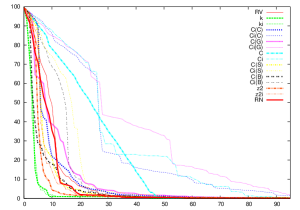
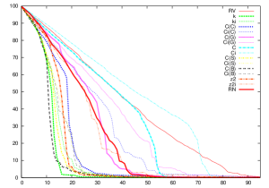
a)                                                                       b)

Figure 1: Attacks on PTNs of (a) Dallas and (b) Paris. Each curve corresponds to a different attack scenario as indicated in the legend, see text. Horizontal axis: percents of removed nodes, Vertical axis: normalized size $S$ of the largest component.

At each step of the attack 1% of the nodes is successively removed following the selection criteria of the given scenarios. The effectiveness of the attack scenarios may be judged by their impact on the value of $S$. As it is clearly seen from Fig. 1, the least effective is the scenario of removing random nodes (RV): it is characterized by the slowest decrease of $S$. Another obvious conclusion is that scenarios based on lists calculated for the initial network (marked by a subscript $i$) appear to be less harmful than those, that are based on recalculated lists. Note however that the difference between ’initial’ and ’recalculated’ scenarios is less evident in the strategies based on the local characteristics, as e.g. the node degree or the number of second nearest neighbours (c.f. curves for $k$, $k_{i}$ and $z_{2}$, $z_{2i}$, respectively). The above difference is even more pronounced for the centrality-based scenarios. A principal difference between attacks on the highest degree nodes on the one hand, and on the highest betweenness nodes on the other hand is that the first quantity is a local, i.e. is calculated from properties of the immediate environment of each node, whereas the second one is global. Moreover, the first strategy aims to remove a maximal number of edges whereas the second strategy aims to cut as many shortest paths as possible. Our analysis shows that the most effective are those scenarios that are either targeted at nodes with the highest values of the node degree $k$, the betweenness centrality $C_{B}$, the next nearest neighbour number $z_{2}$, or the stress centrality $C_{S}$ recalculated after each step of the attack.

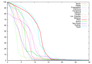
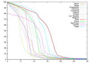
a)                                                                       b)

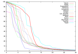
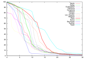
c)                                                                       d)

Figure 2: Four attack scenarios for different PTNs (with recalculation): attacks targeted at nodes of the highest (a) degree $k$, (b) number of second neighbours $z_{2}$, (c) betweenness centrality $C_{B}$, or (d) stress centrality $C_{S}$. Vertical and horizontal axis as in Fig. 1.

Figs. 2, 3 show that the order of destructiveness of these scenarios differ for PTNs of different cities. However, among the scenarios analyzed so far these four appear to be the most effective ones.

Another interesting quantity that we may deduce from Fig. 2 is the vulnerability of the network in terms of the level of destruction at which the largest network component breaks down. We observe that this is strongly correlated to the initial value of the so called Molloy-Reed parameter $\kappa=\overline{z}_{2}/\overline{z}_{1}$ of the unperturbed network. Considering model networks that are randomly built from sets of nodes with given degree distributions it has been shown that the value of $\kappa_{c}=1$ represents the percolation threshold in such networks Cohen03 ; Molloy . A value much larger than $\kappa_{c}$ then indicates a significant distance from the threshold. The values of this parameter for the PTN studied here are: Dallas ($\kappa=1.28$), Istanbul (1.54), Los Angeles (1.59), Hamburg (1.85), London (1.87), Berlin (1.96), Düsseldorf (1.96), Rome (2.02), Sydney (2.54), Hongkong (3.24), São Paolo (4.17), Paris (5.32), Moscow (6.24). Comparing in particular with Fig. 2 a) we find indeed that the higher the initial $\kappa$ value the less vulnerable the network appears to be.

To more precisely define the threshold region for the concentration of removed nodes we observe the behaviour of the maximal $\ell_{\rm max}$ and mean $\overline{\ell}$ shortest path lengths under attack, as shown in Fig. 3. We focus on the recalculated degree scenario (k). Both maximal and average path lengths display similar behaviour: initial growth and then an abrupt decrease when a certain threshold is reached.Obviously, removing the nodes initially increases the path lengths as deviations from the original shortest paths need to be taken into account. Further removing nodes then at some point leads to the breakup of the network into smaller components on which the paths are naturally limited by the boundaries which explains the sudden decrease of their lengths. For the PTN of Paris we observe that this threshold is reached for both $l_{\rm max}$ and $\overline{\ell}$ at the same value of $c_{\rm segm}\simeq 13\%$. The average shortest path on all components of the network, $\langle\ell\rangle$, also possesses a maximum in the same region (for the PTN of Paris it occurs at $c\simeq 13\%$).

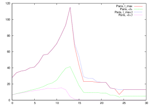
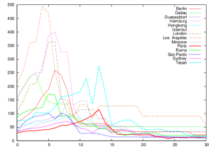
a)                                                                       b)

Figure 3: Highest degree scenario. Horizontal axis as in Fig. 1. (a) Behavior of the maximal and mean shortest path lengths for the Paris PTN calculated for the largest component ($\ell_{\rm max}$, $\overline{\ell}$) and for the whole network ($\ell_{\rm max,f}$, $<\ell>_{\rm f}$). Note a sharp maximum occurs at 13 % of removed nodes (stations) for $\ell_{\rm max}$, $\overline{\ell}$, $\ell_{\rm max,f}$. (b) Behavior of the maximal shortest path length $\ell_{\rm max}$ for the PTNs of different cities.

However, the values of $c_{\rm segm}$ differ for different cities (see Fig. 3,b) and obviously strongly depend on the attack scenario.

As discussed the observed maximum in $\ell_{\rm max}$ (or in $\overline{\ell}$) appears to be a suitable criterion to identify the values of $c$ (or at least the region in $c$), where the segmentation of a network occurs. Other observables which resemble an ’order parameter’, are the above described largest connected component size $S$, Eq.(7), or the average value of the inverse shortest path $\langle\ell^{-1}\rangle$ (6) are less suitable for this purpose because of their rather smooth behaviour. In Fig. 4 we show for PTNs of fourteen cities the behavior of $<\ell^{-l}>$ under attacks following the four most harmful scenarios, i.e. the recalculated highest $k$, $C_{B}$ $z_{2}$ and $C_{S}$ scenarios. Comparing the impact of different attacks scenarios (as seen in particular in Fig. 3, 4) one notices that the apparent relative impact strongly depends on the choice of the observable (e.g. $S$ or $<\ell^{-l}>$).

It is worth to note the statistical origin of the data exposed so far. Different instances of the same scenario may differ to some extent. This is obvious for the random RV or RN scenarios, where the nodes are removed according to a random procedure. However, it remains true even for the attacks following pre-ordered lists of nodes. Obviously, several nodes may have the same value with respect to a given characteristic (e.g. $k$, $z_{2}$,or one of the centrality indices). Then, the choice between these nodes is random. To check the dispersion of the results, Figs. 5, 6 show the results of 10 complete attack sequences for the same scenario. Fig. 5 shows the change in the largest connected component $S$ of the PTNs of Dallas (a), Hongkong (b), and Paris (c) for the random vertex (RV)

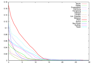
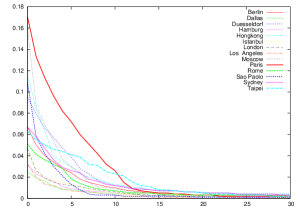
a)                                                                       b)

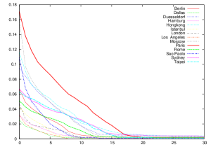
c)                                                                       d)

Figure 4: Behaviour of $<\ell^{-l}>$ for PTNs of different cities under attack following four different scenarios, see text: a) highest $k$, b) highest $C_{B}$, c) highest $z_{2}$, d) highest $C_{S}$. Horizontal axis as in Fig. 1.

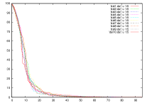
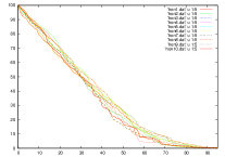
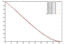
a)                                   b)                                   c) .

Figure 5: Impact and variance of the random vertex (RV) scenario on the normalized size $S$ of the largest component for the PTNs of (a) Dallas, (b) Hongkong, and (c) Paris. Ten curves of different colour indicate different instances of the same scenario for each city. Vertical and horizontal axis as in Fig. 1

scenario. The scatter of the curves in each figure provides an idea about the deviations between individual samples. The figures also clearly show that even attacked randomly, PTNs of different cities may display a range of different behaviour: from the comparatively fast decay of the largest connected component (as in the case of Dallas, Fig. 5a) to very slow, nearly linear decay (as in the case of Paris, Fig. 5c).

The dispersion in the largest connected component size $S$ is much less for sequences of targeted attacks. In Fig. 6 we show the behavior of the largest cluster size and the maximal and mean shortest path lengths for the Paris PTN for ten complete attack sequences following the recalculated degree (k) scenario. Besides a rather narrow scattering of the data for $S$ one notes, that within the current resolution the locations of the maxima in $\ell_{\rm max}$ and $\overline{\ell}$ are very robust.

To give an idea for the numerical values of different characteristics of the PTN as monitored during our analysis we display in Table 1 some data for the PTN of Paris for the recalculated degree scenario for some points of the sequence between the unperturbed network and the vicinity of the threshold (maximum of the shortest path lengths).

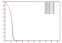
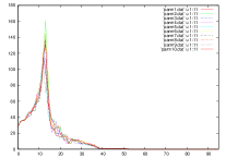
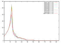
a)                                   b)                                   c)

Figure 6: Ten instances of the recalculated highest degree scenario for the PTN of Paris, observing: a) the largest connected component size $S$, b) the maximal shortest path length $\ell_{\rm max}$, c) the mean shortest path length $\overline{\ell}$. Horizontal axis as in Fig. 1

Table 1: PTN of Paris during an attack sequence following the recalculated degree scenario. $c$: % of removed nodes; $N$: number of remaining nodes; $\overline{k}=\overline{z}_{1}$: mean node degree; $\overline{z}_{2}/\overline{z}_{1}$: ratio of the mean second to the mean first nearest neighbour number; $\ell_{\rm max}$: maximal shortest path length; $\overline{\ell}$: mean shortest path length; $\langle\ell^{-1}\rangle$: mean inverse shortest path length (for all of the remaining network); $\overline{C}_{C}$, $\overline{C}_{G}$, $\overline{C}_{S}$, $\overline{C}_{B}$: mean closeness, graph, stress, and betweenness centralities; $\overline{C}$: mean clustering coefficient; $S$: normalized largest component size.

$c$	$N$	$\overline{k}=\overline{z}_{1}$	$\overline{z}_{2}/\overline{z}_{1}$	$\ell_{\rm max}$	$\overline{\ell}$	$\langle\ell^{-1}\rangle$	$\overline{C}_{C}$	$\overline{C}_{G}$	$\overline{C}_{S}$	$\overline{C}_{B}$	$\overline{C}$	$S$
0	3728	3.73	5.32	28	6.41	0.17	0.004	5.47	38167	10062	0.079	99.87
1	3691	3.25	3.40	34	8.08	0.13	0.003	4.64	40419	12912	0.073	97.85
5	3543	2.52	2.05	41	13.35	0.07	0.002	3.60	50496	20439	0.062	88.81
10	3358	2.00	1.43	70	24.84	0.03	0.002	2.02	53654	30406	0.044	68.45
12	3284	1.84	1.25	93	39.44	0.01	0.001	1.42	56218	36097	0.036	50.40
13	3247	1.77	1.19	115	41.49	0.01	0.003	1.21	31803	18404	0.039	24.41
14	3210	1.70	1.13	67	29.69	0.00	0.008	1.90	11915	6598	0.022	12.37

4 Conclusions

In this paper we reported on some results concerning the behavior of PTNs under attacks. Similar to other real-world and model complex networks Albert00 ; Tu00 ; Jeong00 ; Sole01 ; Jeong01 ; Holme02 , the PTNs manifest very different behaviour under attacks of different scenarios. With some notable exceptions they appear to be robust to random attacks but more vulnerable to attacks targeted at nodes with particular importance as measured by the values of certain characteristics (the most significant being the first and second neighbour numbers, as well as the betweenness and stress centralities). The observed difference between attack scenarios based on the initial and the recalculated distributions shows that the network structure changes essentially during the attack sequence. This is necessarily to be taken into account in the construction of efficient strategies for the protection of these network.

As a suitable criterion to identify the level of resilience, i.e. the number of removed nodes that leads to segmentation it is useful to observe the behaviour of the maximal shortest path length $\ell_{\rm max}$. For the majority of PTNs networks we have analyzed here this observable displays a sharp maximum as function of the removed node concentration which indicates the breakup of the network. Other ’order-parameter-like’ variables like the largest connected component size $S$ or the average value of the inverse shortest path $\langle\ell^{-1}\rangle$ are less suitable for this purpose because of their smooth behaviour. Another observation is that in the recalculated highest-degree attack scenario for the segmentation often occurs at a value of $\kappa=\overline{z}_{2}/\overline{z}_{1}\sim 1$ (see e.g. Table 1 for Paris). Although the PTNs are correlated structures, the above estimate resembles the Molloy-Reed Molloy criterion for randomly built uncorrelated networks. Further investigation is needed to understand the mechanisms that lead to higher resilience against random failure as observed e.g. for the Paris network and how this behavior is related to the network architecture.

As mentioned in the introduction, there are different graph representations, also called ‘spaces’, for a given PTN Ferber07a ; Ferber07b ; Sen03 ; Sienkiewicz05a . These will also lead to different connectivity relations and path lengths between nodes. The resilience of PTNs in these more general ‘spaces’ will be discussed elsewhere Ferber07c .

References

- (1) M. E. J. Newman: SIAM Review 45, 167 (2003); R. Albert, A.-L. Barabási: Rev. Mod. Phys. 74, 47 (2002); S. N. Dorogovtsev, S. N. Mendes: Evolution of Networks, (Oxford University Press, Oxford, 2003); Yu. Holovatch, A. Olemskoi, C. von Ferber et al.: J.Phys. Stud. 10, 247 (2006)
- (2) J. W. Essam: Rep. Prog. Phys. 43, 833 (1980); D. Stauffer, A. Aharony: Introduction to Percolation Theory, (Taylor & Francis, London, 1991)
- (3) C. von Ferber, T. Holovatch, Yu. Holovatch, V. Palchykov: Physica A 380, 585 (2007)
- (4) C. von Ferber, T. Holovatch, Yu. Holovatch, V. Palchykov: Modeling Metropolis Public Transport. In Traffic and Granular Flow ’07. Springer (2007)
- (5) R. Albert, H. Jeong, A.-L. Barabási: Nature (London) 406, 378 (2000)
- (6) Y. Tu: Nature (London) 406, 353 (2000)
- (7) H. Jeong, B. Tombor, R. Albert, Z. N. Oltvai, A.-L. Barabási: Nature (London) 407, 651 (2000)
- (8) R. V. Solé, J. M. Montoya: Proc. R. Soc. Lond. B 268, 2039 (2001)
- (9) H. Jeong, S. P. Mason, A.-L. Barabási, Z. N. Oltvai, Nature (London) 411, 41 (2001)
- (10) R. Cohen, K. Erez, D. ben-Avraham, S. Havlin: Phys. Rev. Lett. 85, 4626 (2000)
- (11) D. S. Callaway, M. E. J. Newman, S. H. Strogatz, D. J. Watts: Phys. Rev. Lett. 85, 5468 (2000)
- (12) A.-L. Barabási, R. Albert: Science 286, 509 (1999); A.-L. Barabási, R. Albert, H. Jeong: Physica A 272, 173 (1999)
- (13) A. Broder, R. Kumar, F. Maghoul, et al.: Comput. Netw. 33, 309 (2000)
- (14) M. Girvan, M. E. J. Newman: Proc. Natl. Acad. Sci. USA 99, 7821-7826 (2002)
- (15) P. Holme, B. J. Kim, C. N. Yoon, S. K. Han: Phys. Rev. E 65, 056109 (2002)
- (16) R. Guimera, L. A. N. Amaral, Eur. Phys. J. B 38, 381 (2004)
- (17) R. Guimera, S. Mossa, A. Turtschi, L.A.N. Amaral: Proc. Nat. Acad. Sci. USA 102, 7794 (2005)
- (18) C. von Ferber, T. Holovatch, Yu. Holovatch: in preparation
- (19) P. Sen, S. Dasgupta, A. Chatterjee et al.: Phys. Rev. E 67, 036106 (2003)
- (20) J. Sienkiewicz, J. A. Holyst: Phys. Rev. E 72, 046127 (2005)
- (21) U. Brandes: J. Math. Sociology, 25, 163 (2001)
- (22) R. Cohen, S. Havlin, D. ben-Avraham Phys. Rev. Lett. 91, 247901 (2003)
- (23) M. Molloy, B. A. Reed: Random Struct. Algorithms 6(2/3), 161 (1995); M. Molloy, B. Reed, Combinatorics, Probability and Computing 7, 295 (1998)