Modeling Metropolis Public Transport

Abstract

We present results of a survey of public transport networks (PTNs) of selected 14 major cities of the world with PTN sizes ranging between 2000 and 46000 stations and develop an evolutionary model of these networks. The structure of these PTNs is revealed in terms of a set of neighbourhood relations both for the routes and the stations. The networks defined in this way display distinguishing properties due to the constraints of the embedding 2D geographical space and the structure of the cities. In addition to the standard characteristics of complex networks like the number of nearest neighbours, mean path length, and clustering we observe features specific to PTNs. While other networks with real-world links like cables or neurons embedded in two or three dimensions often show similar behavior, these can be studied in detail in our present case. Geographical data for the routes reveal surprising self-avoiding walk properties that we relate to the optimization of surface coverage. We propose and simulate an evolutionary growth model based on effectively interacting self-avoiding walks that reproduces the key features of PTN.

1 Introduction

Urban public transport networks (PTNs) share general features of other transportation networks like airport, railroad networks, power grids, etc. Newman03 . The most obvious common features are their embedding into a 2D space, evolutionary growth, and optimization. The evolution of specific local transportation networks is closely related to that of the town or region in which they are embedded. However, statistically, some general overall features such as their fractal dimensions have been observed Benguigui . Modeling different aspects of transportation network structure and functioning helps to understand and optimize various processes that occur on these networks as well as to improve their planning. In this paper, we will consider a PTN from the point of view of complex network theory Newman03 ; Albert02 ; Dorogovtsev03 ; Holovatch06 quantifying statistical features of their structure and proposing a model that reproduces their key features. To exemplify these, we survey the empirical analysis of PTNs of 14 major cities of the world (see Refs. Ferber07a ; Ferber07b for more details). While the empirical analysis of PTNs of different cities has been subject of several studies Marchiori00 ; Latora01 ; Latora02 ; Seaton04 ; Ferber05 ; Sienkiewicz05a ; Ferber07a ; Xu07 ; Holovatch07 (see Sec. 2), we are not aware of previous attempts to specifically model the network evolution of a PTN in the way we propose here. The set-up of the paper is as follows: in the next section we discuss common features of PTNs and list some numbers that quantify these features; section 3 we describe our model for PTN evolution and give supporting arguments; in section 4 we compare some characteristics of real and simulated PTNs; conclusions and an outlook are given in section 5.

2 Empirical analysis of PTNs: statistical properties

A distinct feature of our study is that we interpret the PTN as a network of all means of public transport (buses, trams, subway, etc.) offered in a given city. Several previous studies have analyzed specific sub-networks of PTNs. The Boston Marchiori00 ; Latora01 ; Latora02 ; Seaton04 an Vienna Seaton04 subway networks may serve as examples. However, each particular sub-network (e.g. the network of buses, trams, or subways) is not a closed system: it is a subgraph of a wider transportation system of a city, or as we call it here, of a PTN. Therefore to understand and describe the properties of transport in a city it is important to deal with the complete PTN, not restricting the analysis to specific parts. Indeed, extending the restricted subway network to the “subway + bus” network drastically changes the network properties, as it was shown for Boston Latora01 ; Latora02 .

Another important quantity that certainly restricts the reliability of grneralizations drawn from trends observed for specific PTNs of different cities is the statistics, i.e. the size of the observed PTNs. The numbers of stations $N$ in the PTNs analyzed so far ranged from several decades (subway networks of Boston, $N=124$ Latora02 , and Vienna, $N=76$ Seaton04 ) to several thousands as in the PTN analysis of 22 Polish cities with up to 2811 stations Sienkiewicz05a or bus-transport networks of three Chinese cities with up to $N=3938$ stations. In our sampling Ferber05 ; Ferber07a we have chosen PTNs of 14 major cities of the world of various size with $N$ ranging from 1544 (Düsseldorf) to 46244 (Los Angeles), see Table 1.

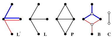
Figure 1: Different representations of a PTN. $\mathbb{L}^{\prime}$-space: nodes correspond to stations, links show different routes. $\mathbb{L}$-space: the same as $\mathbb{L}^{\prime}$ but multiple links are reduced to single ones. $\mathbb{P}$-space: any two stations (nodes) are connected when they are serviced by a common route. $\mathbb{B}$-space: routes (open discs) are linked to those stations (filled discs) that they service. $\mathbb{C}$-space: nodes correspond to routes, links show that two routes share a common station. Note that by keeping multiple links in $\mathbb{P}$ and $\mathbb{C}$ one may also define $\mathbb{P}^{\prime}$ and $\mathbb{C}^{\prime}$-spaces.

Here, we define different graph representations (‘spaces’) for a given PTN in terms of nodes (vertices) and links (edges) as illustrated in Fig. 1. The primary network topology is defined by a set of routes each servicing an ordered series of given stations, see the sketch labeled $\mathbb{L}^{\prime}$ in Fig. 1 Based on this we define a graph ($\mathbb{L}$-space) representing each station by a node and linking any two that are served consecutively by at least one route. More generally linking any two stations serviced by a common route we define the $\mathbb{P}$-space Sen03 ; Sienkiewicz05a representation. The interrelation of the routes in turn is described by a complementary $\mathbb{C}$-space representation where now the nodes represent routes and linking any two that service a common station. From Fig. 1 it is easy to verify, that the last two representations correspond to one-mode projections of a bipartite $\mathbb{B}$-space represenation with nodes of two types, representing either a station or a route linking each route with all stations it services.

Table 1: PTN characteristics in $\mathbb{L}$- and $\mathbb{P}$- representations, see text for definitions. $N$: number of stations, $M$: number of routes, the scale $\hat{k}$ or the exponent $\gamma$ of fits to the node degree distribution $p(k)$ to the laws (1) or (2) respectively, $\mathcal{C}$: ratio of the mean clustering coefficient to its random graph value, maximal $\hat{\ell}$, and mean $\overline{\ell}$ shortest path length. Characteristics in $\mathbb{P}$-space representations are indicated by a subscript ‘p’. See Refs. Ferber07a ; Ferber07b for more data and sources.

City	$N$	$M$			$\mathcal{C}$	$\mathcal{C}_{\rm p}$	$\hat{\ell}$	$\overline{\ell}$	$\hat{\ell}_{\rm p}$	$\overline{\ell_{\rm p}}$
Berlin	2996	218	$\hat{k}$=1.24	$\hat{k}_{\rm p}$=38.5	52.85	42.03	68	18.61	5	2.93
Dallas	6571	131	$\gamma$=4.99	$\hat{k}_{\rm p}$=76.9	17.26	63.00	269	85.84	10	3.78
Düsseldorf	1544	124	$\hat{k}$=1.12	$\hat{k}_{\rm p}$=58.8	22.45	20.97	56	13.18	5	2.58
Hamburg	8158	708	$\hat{k}$=1.47	$\hat{k}_{\rm p}$=55.6	262.92	133.99	158	39.74	11	4.79
Hong Kong	2117	321	$\hat{k}$=2.60	$\hat{k}_{\rm p}$=125.0	58.98	12.51	60	11.11	4	2.26
Istanbul	4043	414	$\gamma$=4.04	$\hat{k}_{\rm p}$=71.4	41.40	41.54	131	29.69	6	3.09
London	11012	2005	$\gamma$=4.58	$\gamma_{\rm p}$=4.39	326.17	90.00	107	26.68	6	3.26
Los Angeles	46244	1893	$\gamma$=4.88	$\gamma_{\rm p}$=3.92	588.44	427.06	247	43.55	14	4.60
Moscow	3755	679	$\hat{k}$=2.12	$\hat{k}_{\rm p}$=50.0	128.23	41.93	28	7.08	5	2.52
Paris	4003	232	$\gamma$=2.61	$\gamma_{\rm p}$=3.70	85.90	71.75	47	7.22	5	2.79
Rome	6315	681	$\gamma$=4.39	$\hat{k}_{\rm p}$=45.5	68.61	76.93	93	29.64	8	3.58
São Paolo	7223	998	$\gamma$=2.72	$\hat{k}_{\rm p}$=200.0	268.83	38.32	33	10.34	5	2.66
Sydney	2034	596	$\gamma$=3.99	$\hat{k}_{\rm p}$=38.5	81.62	34.92	35	12.76	7	3.03
Taipei	5311	389	$\hat{k}$=1.75	$\hat{k}_{\rm p}$=200.0	186.23	15.38	74	20.86	6	2.35

In our analysis, we are interested in different features of the PTN as measured when represented in the above defined spaces. It is worth to mention here, that these standard network characteristics measured in different spaces turn out to be specific of practical value in judging about the quality of public transport in a given city. The particular quantities we analyze here are the maximal and mean shortest path length $\hat{\ell}$ and $\overline{\ell}$, the clustering coefficient $C$, and the betweenness $C_{B}$; for definitions see Ref. attack in this volume. Table 1 gives some of these quantities for the cities analyzed in $\mathbb{L}$- and $\mathbb{P}$- representations. One can see that the above networks are highly clustered small worlds characterized by small shortest path lengths and large ratios $\mathcal{C}$ of the mean clustering coefficient relative to its value $C_{ER}=2M/N^{2}$ on a random graph with the same numbers of nodes $N$ and links $M$.

To classify the node degree distributions $p(k)$ we performed fits to both an exponential function

$$p(k)=Ae^{-k/\hat{k}},$$ (1)

as well as to a power law:

$$p(k)=Bk^{-\gamma}.$$ (2)

The result of the better fit together with the value of the fit parameters $\hat{k}$ or $\gamma$ are shown in table 1. One can see that the $\mathbb{L}$-space node degree distribution of a part of these PTNs (8 out of 14) is governed by power laws, indicating scale-free properties. For the PTNs of several cities, this fact has also been described in Refs. Ferber05 ; Sienkiewicz05a . The remarkable feature of the data shown in table 1 is that some PTNs (3 out of 14) show scale-free behavior even in $\mathbb{P}$-space. As examples compare the degree distributions $p(k)$ of the PTNs of Paris and Sydney in Fig. 2. Whereas the Paris PTN is scale-free both in $\mathbb{L}$- and $\mathbb{P}$-space, the PTN of Sydney is scale-free in $\mathbb{L}$-space only. Note that to reduce the noise in the data we plot the $\mathbb{P}$-space cumulative degree distribution

$$P(k)=\sum_{q=k}^{\infty}p(q).$$ (3)

Figure 2: Node degree distributions for Paris (first row) and Sydney (second row) PTNs. Left column: degree distributions $p(k)$ in $\mathbb{L}$-space. Right column: cumulative degree distributions (3) in $\mathbb{P}$-space.

In Fig. 3 plot the mean betweenness value $C_{B}(k)$ (see attack in this volume) as function of the node degree $k$ in in $\mathbb{C}$-, $\mathbb{L}$-, $\mathbb{P}$-, and $\mathbb{B}$-spaces (similar behaviour is found for the networks of other cities). One definitely sees a pronounced correlation and a tendency for power-law behaviour: a phenomenon observed previously for several other networks Sienkiewicz05a ; Vazquez02 ; Goh03 .

Figure 3: Betweenness-degree correlations for Paris PTN in $\mathbb{C}$-, $\mathbb{L}$-, $\mathbb{P}$-, and $\mathbb{B}$-spaces.

In addition to the standard characteristics of complex networks discussed above, one can introduce some characteristics which are specific to PTNs. One of them is due to the fact that very often several routes go in parallel and pass $L$ consecutive stations. In particular, the notion of harness was introduced in Ref. Ferber07a to quantify this behaviour. In Fig. 4 we show the harness distribution $P(L,R)$: the number of sequences of $L$ consecutive stations that are serviced by $R$ parallel routes for the PTNs of Paris (a) and of Sydney (b). The log-log plot indicates scale free properties of this distribution. We have found similar behaviour for the majority of the cities under consideration.

a)                                   b)                                   c)

Figure 4: Harness distribution for Paris (a), for Sydney (b), and for a simulated city (c).

Following this analysis of PTNs of different cities of the world and having at hand the numerical data on different features of these networks, let us propose a model, that may reproduce most of these features. In particular, the model should be capable to discriminate between different types of behaviour observed so far in PTNs (an example may be the exponential and power-law node degree distributions for $p(k)$ observed for different cities).

3 Evolutionary Model of PTNs

To model the properties of PTNs we have proposed Ferber07a an evolutionary growth model for these networks along the following lines: We model the grid of streets by a square lattice and allow every lattice site $\vec{r}$ (street corner) to be a potential station visited by say $k(\vec{r})$ routes. The routes are modeled as self-avoiding walks (SAWs) on this lattice. The rules of our model are the following:

• First route: construct a SAW of length $n$ starting at an arbitrary site.

• Subsequent routes:

  • (i) choose a terminal station on lattice site $\vec{r}$ with probability $q\propto k(\vec{r})+a$;

  • (ii) choose a subsequent station of this route at a neighboring site $\vec{r}^{\prime}$ with probability $q\propto k(\vec{r}^{\prime})+b$;

  • (iii) repeat step (ii) until the walk has reached $n$ stations, in case of self-intersection discard the walk and restart with step (i).

• Repeat step 2 until $M$ routes are created.

a)                                   b)

c)                                   d)

Figure 5: Different simulated PTN maps of ’cities’ of size $300\times 300$ with $M=500$ routes of $n=50$ stations each. a): $a=0.0001,b=1$, b): $a=0.001,b=1$, c): $a=0,b=0.1$, d): $a=0,b=0.5$.

The above rules resemble the preferential attachment growth rule prefattach favoring high-degree nodes when linking new nodes to a network. The principal difference of our algorithm is that at each step (2ii) we link an existing station to a neighboring site which does not need to be empty. New stations are then only added at the frontier of the PTN cluster while high degree nodes (hubs) accumulate at its center. The choice of a SAWs to model the routes may seem odd at first sight. however, the fractal dimensions measured in PTNs Benguigui ; Ferber07a are compatible with 2D SAW behaviour for the routes and it is obvious that a single PTN route very seldom intersects itself. Moreover, the scaling properties of SAWs on disordered lattices do not change, provided the disorder is short-range correlated saw . In our application this means, that even the presence of certain geographical constraints and deviations from the square lattice still allow for a SAW description of a PTN route.

The above described generating procedure results in a simulated PTN of $M$ routes, each consisting of $n$ stations. In Fig. 5 we show several typical PTN configurations of simulated cities on a $300\times 300$ square lattice with $M=500$, $n=50$ and different values of $a$ and $b$. The parameters $a$ and $b$ allow to discriminate between different regimes of the network evolution. Setting $a=0$ limits every new route to start from an already existing station. On the contrary, for $a\neq 0$, the terminal station of a new route may be situated at any lattice site. Therefore, increasing $a$ allows for PTNs that consist of more than one component (c.f. Figs. 5a and 5b). The parameter $b$ on the other hand tunes the evolution of the routes: a small value of $b$ forces the routes to propagate in parallel (harnessed) while increasing $b$ results in routes that cover more sites of the lattice (see Figs. 5c, 5d correspondingly). In the next section we will investigate how the numerical characteristics of the modeled PTNs correspond to those observed for real cities.

4 Simulation Results

Postponing a more detailed analysis of the numerical simulations based on the model of section 3 to a separate publication Ferber07b , we focus here on several principal features of PTNs and deomstrate how they are reproduced by our model. One of them is the behaviour of the node degree distribution $p(k)$. As it was shown in section 2, the behaviour of this function varies for PTNs of different cities. In $\mathbb{L}$-space one often observes $p(k)$ to be of a power-law type (2) Ferber05 ; Sienkiewicz05a ; Xu07 ; Ferber07a , however sometimes it is governed by an exponential decay (1). Moreover, recently these two types of behaviour were also observed in $\mathbb{P}$-space Ferber07a . A distinguished feature of our model is that depending on the values of the evolution parameters $a,b$ it discriminates between a power-law and an exponential $p(k)$ in $\mathbb{P}$-space. Note that on the square lattice the $\mathbb{L}$-space degrees are limited to $k\leq 4$ ruling out such an analysis. As an example, in Fig. 6 we show the cumulative node degree distribution $P(k)$, see Eq. 3, for PTNs of two simulated cities in the $\mathbb{P}$-space. Changing the value of parameter $b$ for fixed $a$ one passes from an exponential (a straight line in the log-linear plot in Fig. 6a) to a power-law regime (a straight line in the log-log plot in Fig. 6b).

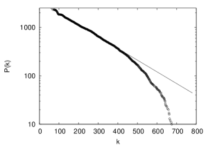
a)                                               b)

Figure 6: $\mathbb{P}$-space cumulative degree distribution $P(k)$ for different simulated cities of $300\times 300$ sites with $M=500$ and $n=50$. a) $a=0$, $b=0.5$: exponential in $\mathbb{P}$-space, b) $a=0$, $b=0.1$: power law in $\mathbb{P}$-space.

Another specific feature of real world PTNs that is nicely reproduced by our model is the harnessing effect. In Fig. 3c we show the harness distribution $P(L,R)$ for the PTN of a simulated city on $300\times 300$ sites with $M=500$ and $n=50$ at $a=0$, $b=0.5$ in comparison with the same quantity for the PTNs of Paris (Fig. 3a) and of Sydney (Fig. 3b). Again, as in the case of real-world PTNs one may speculate about power-law behaviour. Note however, that neither for the node degree nor for the harness distribution we so far find a simple relation between the exponents that may govern the scaling and the model evolution parameters $a,b$. Finally, let us compare the betweenness-degree correlation. In the same way as for the PTN of Paris (Fig. 3), we plot this function in Fig. 7 for different representations for a simulated city of $300\times 300$ sites with $M=500$ and $n=50$ for the evolution parameters $a=0,b=0.5$. One can see an overall qualitative agreement between the behaviour observed for the real-world network and the simulated one (for $\mathbb{L}$ see discussion above). In this context it is worth to mention that the simultaneous use of different representations (spaces) serves as a useful tool to quantify the correspondence and differences between real word networks as well as simulated ones.

Figure 7: Betweenness-degree correlation for the simulated city of $300\times 300$ sites with $M=500$ and $n=50$ in $\mathbb{C}$-, $\mathbb{L}$-, $\mathbb{P}$-, and $\mathbb{B}$-spaces. $a=0,b=0.5$.

5 Conclusions and outlook

The small-world properties of public transport networks are an everyday experience: it is easy to reach almost any given place in a city with only a small number of changes of transport (from table 1 it follows e.g. that the connection between any two stations in Paris implies on average $\overline{\ell_{\rm p}}-1=1.8$ changes), the scale-free properties of these networks are not that evident. Even more, scale free properties for these networks have sometimes been doubted. The results of our empirical analysis of PTNs of 14 major cities of the world Ferber07a ; Holovatch07 ; Ferber07b together with the empirical data for several other cities Marchiori00 ; Latora01 ; Latora02 ; Seaton04 ; Ferber05 ; Sienkiewicz05a ; Xu07 however give a strong evidence of the fact that scale-free behaviour emerges in many PTNs. Apart from our model we currently cannot give more general arguments for this this behaviour. Furthermore, not all PTNs seem to exhibit power-law node degree distributions, as some display rather an exponential decay of $p(k)$, see Table 1. Inspired by this observation we developed an evolutionary model of self-avoiding walks on 2D lattice which discriminates between the above types of behaviour and recovers a number of other basic features of the PTNs. The model applies the idea of the preferential attachment scenario prefattach , however with specific differences to that standard scenario: as far as the PTNs constitute an example of ever evolving networks, such a mechanism is not unlikely to play a role in their growth. In more general terms, scale-free networks have been shown in certain situation to minimize both the effort for communication and the cost for maintaining connections optimization ; Gastner04 . Similar optimization was shown to lead to the small world properties Mathias01 and used to explain the appearance of power laws zipfoptimal . Therefore one may expect the observed scale-free behaviour of PTNs to naturally emerge from obvious optimization objectives followed in their design.

One of the specific features of the PTNs we have analyzed is the harnessing effect: very often several routes go in parallel and pass together several consecutive stations. While other networks with real-world links like cables or neurons embedded in two or three dimensions often show similar behavior, these can be studied in detail in our present case. Our empirical analysis of the harness distribution that quantifies this behavior indicates power-law behaviour. The same behaviour is inherently recovered by our model. We found that a useful tool to classify PTNs as well as to find correspondence between real-world and simulated PTNs is a comparison of the observables in different representations (‘spaces’). Furthermore, the standard network characteristics as represented in different spaces turn out to be natural measures for the quality of public transport in a city.

Of the many interesting further questions that are related to this study let us only mention the vulnerability of PTNs to random failures and targeted attacks (see our contribution attack on this subject in this volume) as well as the correlation between the topological properties of a PTN and its geographical embedding.

References

- (1) M. E. J. Newman: SIAM Review 45, 167 (2003)
- (2) L. Benguigui: J. Phys. I France 2, 385 (1992); L. Benguigui, M. Daoud: Geogr. Analysis 23, 362 (1991)
- (3) R. Albert, A.-L. Barabási: Rev. Mod. Phys. 74, 47 (2002)
- (4) S. N. Dorogovtsev, S. N. Mendes: Evolution of Networks, (Oxford University Press, Oxford, 2003)
- (5) Yu. Holovatch, A. Olemskoi, C. von Ferber et al.: J.Phys. Stud. 10, 247 (2006)
- (6) M. Marchiori, V. Latora: Physica A 285, 539 (2000)
- (7) V. Latora, M. Marchiori: Phys. Rev. Lett. 87, 198701 (2001)
- (8) V. Latora, M. Marchiori: Physica A 314, 109 (2002)
- (9) K. A. Seaton, L. M. Hackett: Physica A 339, 635 (2004)
- (10) C. von Ferber, Yu. Holovatch, V. Palchykov: Condens. Matter Phys. 8, 225 (2005)
- (11) J. Sienkiewicz, J. A. Holyst: Phys. Rev. E 72, 046127 (2005)
- (12) X. Xu, J. Hu, F. Liu, L. Liu: Physica A 374, 441 (2007)
- (13) C. von Ferber, T. Holovatch, Yu. Holovatch, V. Palchykov: Physica A 380, 585 (2007)
- (14) C. von Ferber, T. Holovatch, Yu. Holovatch: Attack Vulnerability of Public Transport Networks. In Traffic and Granular Flow ’07. Springer (2007)
- (15) T. Holovatch: Modeling statistical properties of public transport networks. Diploma Thesis, Ivan Franko National University of Lviv, Lviv, Ukraine (2007)
- (16) C. von Ferber, T. Holovatch, Yu. Holovatch, V. Palchykov: in preparation
- (17) P. Sen, S. Dasgupta, A. Chatterjee et al.: Phys. Rev. E 67, 036106 (2003)
- (18) A. Vázquez, R. Pastor-Satorras, A. Vespignani: Phys. Rev. E 65, 066130 (2002)
- (19) K.-I. Goh, E. Oh, B. Kahng, et al.: Phys. Rev. E 67, 017101 (2003)
- (20) A.-L. Barabási, R. Albert: Science 286, 509 (1999); A.-L. Barabási, R. Albert, H. Jeong: Physica A 272, 173 (1999)
- (21) A.B. Harris: Z. Phys. B 49, 347 (1983); Y. Kim: J. Phys. C 16, 1345 (1983)
- (22) R. Ferrer i Cancho, R. V. Solé: e-print cond-mat/0111222; S. Valverde, R. Ferre Cancho, R. V. Solé: Europhys. Lett. 60, 512 (2002); R. Ferrer i Cancho, R. V. Solé. In: Statistical mechanics of Complex Networks, ed by R. Pastor-Satorras, M. Rubi, A. Diaz-Guilera (Lecture Notes in Physics Vol 625, Springer, Berlin, 2003), p. 114.
- (23) M. T. Gastner, M. E. J. Newman: Eur. Phys. J. B 49, 247 (2006)
- (24) N. Mathias: Phys. Rev. E 63, 021117 (2001)
- (25) R. Ferrer i Cancho, R. V. Solé: Proc. Natl. Acad. Sci. USA. 100, 788 (2003); R. Ferrer i Cancho: Physica A 345, 275 (2005)