Physics of Interpulse Emission in Radio Pulsars

Abstract

The magnetized induced Compton scattering off the particles of the ultrarelativistic electron-positron plasma of pulsar is considered. The main attention is paid to the transverse regime of the scattering, which holds in a moderately strong magnetic field. We specifically examine the problem on induced transverse scattering of the radio beam into the background, which takes place in the open field line tube of a pulsar. In this case, the radiation is predominantly scattered backwards and the scattered component may grow considerably. Based on this effect, we for the first time suggest a physical explanation of the interpulse emission observed in the profiles of some pulsars. Our model can naturally account for the peculiar spectral and polarization properties of the interpulses. Furthermore, it implies a specific connection of the interpulse to the main pulse, which may reveal itself in the consistent intensity fluctuations of the components at different timescales. Diverse observational manifestations of this connection, including the moding behavior of PSR B1822-09, the peculiar temporal and frequency structure of the giant interpulses in the Crab pulsar, and the intrinsic phase correspondence of the subpulse patterns in the main pulse and the interpulse of PSR B1702-19, are discussed in detail. It is also argued that the pulse-to-pulse fluctuations of the scattering efficiency may lead to strong variability of the interpulse, which is yet to be studied observationally. In particular, some pulsars may exhibit transient interpulses, i.e. the scattered component may be detectable only occasionally.

1 INTRODUCTION

The profiles of some pulsars include the component usually called interpulse (IP), which is separated from the main pulse (MP) by approximately a half of the pulsar period. The IPs may be as weak as a few per cent of the MP and typically have much steeper spectra, being most pronounced at low frequencies (Bruck & Ustimenko, 1977). In several pulsars, the IP is connected to the MP with a barely distinguishable emission bridge, and the low-level emission may extend over practically the whole pulse period (e.g. Hankins & Cordes, 1981). In general, the IP is located not exactly midway between the successive MPs, but may be shifted by up to a few tens degrees toward earlier or later pulse phases. In case of still larger shifts the IP is rather referred to as the postcursor or the precursor to the MP (e.g. Weisberg et al., 1981; Rankin & Rathnasree, 1997; Kramer et al., 1998). Note that the pulse profile may contain a few such components at once. For example, the Crab pulsar has a total of six components outside of the MP, which exhibit pronounced frequency evolution (Moffett & Hankins, 1996; Cordes et al., 2004). The emission components outside of the MP are characteristic of the short-period pulsars, $P\lesssim 0.6$ s (Manchester & Lyne, 1977), and especially of the millisecond pulsars (Kramer et al., 1998). The IPs are met in $\sim 2\%$ of the normal pulsars and $\sim 40\%$ of the millisecond ones.

As a rule, the IP separation from the MP does not change with frequency (Hankins & Fowler, 1986). This contrasts with the spectral behaviour of the component separations inside the MP, which are known to increase with wavelength, signifying the overall broadening of the emission cone. Besides that, the IPs usually have distinctive polarization characteristics, showing higher precentage of linear polarizaton and a shallow position angle swing, the position angle itself being not very much different from that of the MP. Although the classical model of rotating vector explains successfully the position angle swing across the MP in a number of pulsars, its application to the profiles with IPs often faces difficulties (e.g. Rankin & Rathnasree, 1997).

The single-pulse observations further reveal the peculiarities of the IP emission. The IP intensity appears modulated at various timescales. Similarly to the MPs, the IPs may exhibit a number of fluctuation phenomena, such as microstructure, subpulse drift, pulse-to-pulse intensity modulation, mode changing, and giant pulses. In PSR B0950+08, the IP shows microstructure comparable with that in the MP (Hankins & Boriakoff, 1981). Recently it has been found that the subpulse patten in the IP of PSR B1702-19 has the same periodicities as that in the MP, and moreover, the two patterns are intrinsically in phase (Weltevrede et al., 2007). This striking result directly testifies to the physical relation between the MP and IP emissions. Some indirect manifestations of such a relation have presumably been known previously. In particular, in PSR B0950+08, a strong MP is followed by a strong IP (Hankins & Cordes, 1981), whereas in PSR B1055-52 a strong IP is followed by a strong MP (Biggs, 1990). In both cases the strong components appear separated by more than a half of the pulse period. It is still obscure whether this peculiar intensity correlation is an artifact of the subpulse drift or not.

Apart from the weak intensity fluctuations of the IP emission similar to those in the MP, occasional strong pulses, with intensities as large as about the MP intensity, can be met in these pulsars at the position of the IP (Hankins & Cordes, 1981; Biggs, 1990). These transient events are so rare that neither the average IP profile nor the above mentioned MP-IP correlation are affected.

In PSR B1822-09, the IP shows quite different fluctuation behaviour, participating in mode changing (Fowler et al., 1981; Fowler & Wright, 1982; Gil et al., 1994). The IP appears pronounced only in the so-called quiet mode, i.e. in the sequence of weak enough pulses. In the bright mode, a strong precursor arises some $20^{\circ}$ ahead of the MP, whereas the IP becomes markedly weaker. Thus, the IP intensity is anticorrelated with both the MP and precursor intensities.

Provided that the giant pulse activity is characteristic of the MP (e.g. in the Crab pulsar and PSR B1937+21), giant pulses can also be met in the IP, though they are not necessarily simultaneous in the two components at a given frequency. In the Crab pulsar, giant MPs and IPs are found to exhibit quite distinct temporal and frequency structures (Eilek & Hankins, 2007). Giant MPs consist of one or several broadband microbursts made up of shorter and narrowband nanoshots ($\delta t\sim 10/\nu$, $\delta\nu/\nu\sim 0.1$). Giant IPs contain microsecond-long trains of proportionally spaced emission bands ($\delta\nu/\nu\sim 0.06$), which are grouped into regular band sets.

In summary, the IP emission is characterized by a number of peculiarities, and at the same time shows diversiform manifestations of its physical connection to the MP. All this calls for theoretical explanation. In the preceding literature, the IPs are interpreted in terms of several geometrical models. One of the models suggests that the IP is emitted from the magnetic pole opposite to that responsible for the MP and the magnetic axis is nearly orthogonal to the rotational axis, in which case the emission from both poles is alternately seen by an observer. This two-pole model can satisfactorily explain the main features of the IP components, except for their physical relation to the MP emission and the continuous emission bridge, which may connect them to the MP. These difficulties are removed in the single-pole models. In the first version of such a model, the MP and IP are identified with the two components of a hollow emission cone under the condition of unusually large angular extent of the cone and/or approximate alignment of the magnetic and rotational axes of a pulsar (Manchester & Lyne, 1977). Although this model naturally explains the emission bridge between the MP and the IP as well as the physical connection of the components, it is not clear why the components so much differ in intensity and their separation does not change with frequency like that between the conal components of the ordinary narrow profiles. Later on Gil (1985) attempted to improve the single-pole model in order to avoid these difficulties. It has been assumed that the two concentric hollow cones, the inner and outer ones, are centered at the magnetic axis, which is almost aligned with the rotational axis. Then the portions of the inner and outer emission cones grazed by the sight line form the MP and the IP in the resultant pulse profile.

Recently Dyks et al. (2005) have suggested a bidirectional model of pulsar emission and applied it to the peculiar profile of PSR B1822-09. In that model, the MP and the precursor originate independently at different altitudes above the same magnetic pole and the precursor emission intermittently reverses its direction to form the IP. This so-called inward emission directed toward the neutron star can be observable provided that the magnetic and rotational axes are nearly orthogonal. The physics underlying the reversal of the emission direction is not specified, but for any conceivable switching mechanism it is difficult to explain the connection of the emission direction to the MP intensity.

In the present paper, we suggest the first physical model of IPs. In contrast to the above mentioned geometrical models, it is aimed at explaining the spectral and polarization peculiarities of the IP emission as well as the nature of the MP-IP connection. Recently we have proposed the physical mechanism of the precursors (Petrova, 2007). It is based on induced scattering of the MP emission into the background. It has been found that in case of a superstrong magnetic field the scattered radiation is directed almost along the field. Then, because of rotational aberration in the scattering region, the scattered component appears in the pulse profile up to $30^{\circ}$ ahead of the MP. In the present paper, we extend the theory of magnetized induced scattering to the case of a moderately strong magnetic field. It will be shown that in this approximation the MP emission is scattered in the direction antiparallel to the ambient magnetic field and may form the profile component roughly midway between the MPs.

The plan of the paper is as follows. In Section 2, we examine the problem on the radio beam scattering into the background in application to pulsars. The properties of the scattered component are compared with the observed features of the IP emission in Section 3. A summary of our model of the IP formation is given in Section 4. Basic formalism of induced scattering in the approximation of moderately strong magnetic field is given in Appendix.

2 TRANSVERSE SCATTERING IN PULSAR MAGNETOSPHERE

2.1 General Considerations

Pulsar magnetospheres contain the ultrarelativistic electron-positron plasma, which streams along the open magnetic lines. The radio emission is believed to originate deep inside the open field line tube, and therefore it should propagate through the plasma flow. As the brightness temperatures of pulsar radio emission are extremely high, the induced scattering off the plasma particles may be substantial. The induced scattering of radio emission by the non-magnetized pulsar wind has been considered by Wilson & Rees (1978). However, inside the magnetosphere of a pulsar, the magnetic field may be strong enough to affect the scattering process considerably. This happens on condition that the radio frequency in the particle rest frame is much less than the electron gyrofrequency, $\omega^{\prime}\equiv\omega\gamma(1-\beta\cos\theta)\ll\omega_{G}\equiv eB/(mc)$ (here $\gamma$ is the particle Lorentz-factor, $\beta$ the velocity in units of $c$, $\theta$ is the angle the incident photon makes with the particle velocity, and the quantities not denoted by primes correspond to the laboratory frame). The magnetized scattering has been studied in a number of papers (e.g. Canuto, 1970; Canuto et al., 1971; Hamada & Kanno, 1974; Blandford & Scharlemann, 1976; Börner & Mészáros, 1979; Ochelkov & Usov, 1983; Chou, 1986).

In the vicinity of the emission region of a pulsar, the regime of magnetized scattering is certainly valid. As the magnetic field strength decreases with distance from the neutron star, $B\propto r^{-3}$, at high enough altitudes $\omega^{\prime}=\omega_{G}$, i.e. the cyclotron resonance takes place. The resonance region typically lies in the outer magnetosphere, and hence the regime of magnetized scattering, $\omega^{\prime}\ll\omega_{G}$, holds over a substantial part of the open field line tube well below the light cylinder.

The pulsar radio emission is believed to be generated at the frequencies of order of the local Lorentz-shifted proper plasma frequency, $\omega\sim\omega_{p}\sqrt{\gamma}$, where $\omega_{p}\equiv\sqrt{4\pi n_{e}e^{2}/m}$ and $n_{e}$ is the plasma number density (but see Melrose & Gedalin, 1999, for the criticism of this point). Hence, in the emission region and its close neighborhood, the scattering is the collective process. The induced scattering of different types of the plasma waves is an important ingredient of various scenarios of the pulsar emission mechanism (e.g. Lominadze et al., 1979; Lyubarskii, 1992, 1993, 1996; Lyutikov, 1998). Besides that, the resultant radio waves may participate in the induced three-wave interactions (Gangadhara & Krishan, 1993; Lyutikov, 1998; Luo & Melrose, 2006). As the plasma number density decreases with the distance from the neutron star, $n_{e}\propto B\propto r^{-3}$, well above the emission region $\omega\gg\omega_{p}\sqrt{\gamma}$, in which case the plasma effects are negligible and the induced scattering is a single-particle process (e.g. Lyutikov, 1998). In the present paper, we dwell on the magnetized induced scattering in the single-particle approximation. Then the incident radiation presents the transverse waves linearly polarized either in the plane of the ambient magnetic field or perpendicularly to this plane.

Actually, there are two regimes of magnetized scattering, the longitudinal and transverse ones (e.g. Blandford & Scharlemann, 1976; Ochelkov & Usov, 1983). As the strength of the external magnetic field tends to infinity, the excited motion of a particle in the field of the incident wave is confined to the magnetic field line. This is a so-called longitudinal scattering. Because of a purely longitudinal motion of the particle in this regime, only the photon states with the polarization in the plane of the ambient magnetic field are involved in the scattering. In case of somewhat weaker magnetic fields, the excited motion of a particle presents a drift in the crossed fields, the electric field of the incident wave and the ambient magnetic field. In case of large enough transverse component of the perturbed particle velocity the character of the scattering changes substantially. In particular, this so-called transverse scattering involves the photons of both polarizations, with the electric vectors in the plane of the magnetic field and perpendicular to this plane. In case of spontaneous scattering of the radiation directed at the angle $1/\gamma\ll\theta\ll 1$ to the magnetic field, the longitudinal regime holds if $\theta\gamma\omega^{\prime}/\omega_{G}\ll 1$, whereas the transverse one on condition that $(\theta\gamma)^{-1}\ll\omega^{\prime}/\omega_{G}\ll 1$ (e.g. Ochelkov & Usov, 1983). For the induced scattering of radio beam into background, which will be studied in the present paper, the condition of switching between the regimes is expected to be somewhat modified, and this question will be examined in detail in Section 2.5.

At the conditions relevant to pulsar magnetosphere, both regimes are believed to be appropriate. Previous studies of magnetized induced scattering in application to pulsars have concentrated on the longitudinal regime (Blandford & Scharlemann, 1976; Lyubarskii & Petrova, 1996; Petrova, 2004a, b, 2007). This process appears efficient, and it may cause a number of observational consequences. In particular, induced longitudinal scattering of the radio beam into the background may account for the low-frequency turnovers in pulsar spectra (Lyubarskii & Petrova, 1996), whereas the scattered component may be identified with the precursor to the MP (Petrova, 2007); the scattering inside the beam results in the photon focusing, which may underlie the formation of microstructure in pulsar profiles (Petrova, 2004a); induced scattering between the two beams of substantially different frequencies and orientations leads to significant intensity redistribution in frequency and can explain giant pulses along with their nanostructure (Petrova, 2004b).

The induced scattering in the transverse regime has been briefly discussed in Blandford & Scharlemann (1976). General formalism of this process is developed in the Appendix of the present paper. The kinetic equations obtained are used to solve the problem of the radio beam scattering into the background. The main motivation of our study is that in contrast to the longitudinal scattering regime, the radiation is believed to be scattered backwards, in the direction antiparallel to the particle velocity. Therefore we suggest the induced transverse scattering as a mechanism underlying the formation of interpulses.

2.2 Statement of the Problem

Let the radio beam pass through the open field line tube of a pulsar and be scattered off the particles of the plasma flow. The radiation of pulsars is known to be highly directional: At any point of the pulsar emission cone it is concentrated into a narrow beam with the opening angle $\lesssim 1/\gamma$, whereas the width of the emission cone itself (which determines the observed pulse width) is typically much larger. Far from the emission region, the radiation propagates quasi-transversely with respect to the ambient magnetic field, $1/\gamma\ll\theta<1$. Therefore one can neglect the beam width and represent the incident radiation by a single wavevector ${\bf k}$ at any point of the scattering region. (Note that at different locations within the pulsar emission cone the wavevector orientations somewhat differ, so that the observed pulse has a non-zero width.)

The rate of induced scattering is known to depend on the particle recoil, i.e. on the difference of the initial and final directions of the photons, and therefore the scattering within the beam is of no interest here. On the other hand, by definition the induced scattering cannot transfer the beam photons into the states where the photon occupation numbers are initially zero. However, the photons can still be subject to induced scattering out of the beam, since some background photons are expected to be always present in space. In particular, they may result from the spontaneous scattering of the beam, which, in contrast to the induced one, provides the photons of any orientation. Although in pulsar case the spontaneous scattering is very inefficient and the scattered photons are too scanty to be detectable (see, e.g., eq.[13] below), they can still stimulate a substantial induced scattering from the radio beam. The beam photons should predominantly undergo induced scattering into the background state ${\bf k_{1}}$, which corresponds to the maximum scattering probability. If the induced scattering is efficient enough, the background radiation in this state may grow significantly and become almost as strong as the initial radio beam.

It should be noted that in the particle rest frame the photon frequency is approximately unchanged in the scattering act. Therefore in the laboratory frame $\omega\eta=\omega_{1}\eta_{1}$. Thus, we examine the problem on induced scattering between the two photon states, ${\bf k}=(2\pi\nu/c,\theta,\phi)$ and ${\bf k_{1}}=(2\pi\nu_{1}/c,\theta_{1},\phi_{1})$, one of which corresponds to the beam and another one to the background state characterized by the maximum scattering probability; the frequencies are related as $\nu\eta=\nu_{1}\eta_{1}$, and the occupation number of the background photons is initially much less than that of the beam photons, $n_{1}\lll n$.

2.3 Analytical Treatment

The kinetic equations describing the rate of the magnetized induced scattering are derived in Appendix (see eqs.[A7]). To proceed further we introduce several simplifications. First of all, as we concentrate on the transverse scattering, only the last terms in the kinetic equations (A7) should be retained. Then these equations can be presented as

$$\frac{{\rm d}n}{{\rm d}r}(i\to j)=\int{\rm d\gamma F(\gamma)}\int\widetilde{a}g^{ij}{\rm d}\Omega_{1},$$ (1)

where

$$\widetilde{a}=\frac{2\hbar k}{mc}r_{e}^{2}n(k)n_{1}(k\eta/\eta_{1})\frac{\omega^{4}\eta^{4}\gamma^{4}}{\omega_{G}^{4}}\frac{\eta-\eta_{1}}{\eta_{1}^{3}}\frac{\eta\gamma^{2}-1}{\beta^{2}\gamma^{5}},$$ (2)

$i,j$ stand for the polarization states of the incident and scattered photons, and

$$g^{BB}=1+\sin^{2}\Delta\phi,$$ (3a)

$$g^{BA}=(1+\cos^{2}\Delta\phi)\frac{(1-\eta_{1}\gamma^{2})^{2}}{\beta^{2}\gamma^{4}\eta_{1}^{2}},$$ (3b)

$$g^{AB}=(1+\cos^{2}\Delta\phi)\frac{(1-\eta\gamma^{2})^{2}}{\beta^{2}\gamma^{4}\eta^{2}},$$ (3c)

$$g^{AA}=(1+\sin^{2}\Delta\phi)\frac{(1-\eta\gamma^{2})^{2}}{\beta^{2}\gamma^{4}\eta^{2}}\frac{(1-\eta_{1}\gamma^{2})^{2}}{\beta^{2}\gamma^{4}\eta_{1}^{2}}-\frac{\sin 2\theta\sin 2\theta_{1}\cos\Delta\phi}{2}.$$ (3d)

One can see that the kinetic equations differ from each other only by the factor $g^{ij}$, which is generally of order unity. (Note the symmetry of $g^{ij}$ with respect to the initial and final photon states). Further, a detailed form of the particle distribution function does not play a crucial role. Therefore we consider a monoenergetic distribution with some characteristic Lorentz-factor of the particles.

It is convenient to replace the photon occupation numbers with the intensities, $i_{\nu}=2h\nu^{3}n({\bf k})/c^{2}$ and $i_{\nu_{1}}=2h\nu_{1}^{3}n_{1}({\bf k_{1}})/c^{2}$, and making use of their delta-functional angular distributions to integrate the kinetic equation over the solid angle. Then we come to the following system of equations for the spectral intensities of the beams $I_{\nu,\nu_{1}}\equiv\int i_{\nu,\nu_{1}}{\rm d}\Omega_{1}$:

$$\frac{{\rm d}I_{\nu}}{{\rm d}r}=-ag^{ij}I_{\nu}I_{\nu_{1}},$$

$$\frac{{\rm d}I_{\nu_{1}}}{{\rm d}r}=ag^{ij}I_{\nu}I_{\nu_{1}},$$ (4)

where

$$a=\frac{4n_{e}r_{e}^{2}}{m\gamma^{3}\nu^{2}\theta^{4}}\frac{\nu^{\prime^{4}}}{\nu_{G}^{4}}(\eta_{1}-\eta),$$ (5)

and $n_{e}\equiv\int F(\gamma){\rm d}\gamma$ is the particle number density. Obviously, the radio beam intensity $I_{\nu}$ decreases because of the photon scattering to the state with $\theta_{1}>\theta$ and the maximum scattering probability corresponds to $\theta_{1_{\rm max}}=\pi$ and $\nu_{1}=\nu\theta^{2}/4\ll\nu$. Note that in this situation the azimuthal angle $\phi_{1}$ is of no interest.

The system (4) has the following solution (see, e.g., Petrova, 2004b):

$$I_{\nu}=\frac{I(I_{\nu}^{(0)}/I_{\nu_{1}}^{(0)})\exp(-Iag^{ij}r)}{1+(I_{\nu}^{(0)}/I_{\nu_{1}}^{(0)})\exp(-Iag^{ij}r)},$$

$$I_{\nu_{1}}=\frac{I}{1+(I_{\nu}^{(0)}/I_{\nu_{1}}^{(0)})\exp(-Iag^{ij}r)},$$ (6)

where

$$I\equiv I_{\nu}+I_{\nu_{1}}={\rm const}$$ (7)

is the first integral. Thus, in our approximate consideration the induced scattering results in the net intensity transfer of the radio beam intensity into the background. Of course, an exact treatment of the problem taking into account the complete rather than approximate cross-sections would show that the total intensity $I$ somewhat decreases, the energy being deposited to the scattering particles, and the number of photons $n+n_{1}$ is conserved instead of the intensity $n\nu+n_{1}\nu_{1}$. One can see that as a significant fraction of photons comes to the background state, $n_{1}\sim n^{(0)}\ll n$, the corresponding intensity is $n_{1}\nu_{1}\sim n^{(0)}\nu\theta^{2}<n^{(0)}\nu$. Hence, of the original energy of the radio beam, $n^{(0)}\nu$, about $\theta^{2}n^{(0)}\nu$ is transferred to the background state and $\sim(1-\theta^{2})n^{(0)}\nu$ is gained by the particles. Although $\theta\lesssim 1$, the background intensity grows drastically (cf. eq.[13] below), and the intensity transfer between the two states greatly dominates the evolution of the total intensity $I$. In our treatment, the latter is ignored and the intensity of the efficiently growing component is intended to be roughly comparable with the original radio beam intensity or at least be above the detection level.

According to equation (6), the efficiency of intensity transfer is characterized by the quantity $\Gamma=Iag^{ij}r$. Provided that $\Gamma\gtrsim 1$ the background intensity grows exponentially, $I_{\nu_{1}}\approx I_{\nu_{1}}^{(0)}\exp(\Gamma)$, but still remains much less than the original radio beam intensity, and, correspondingly, $I_{\nu}\approx I_{\nu}^{(0)}$. A significant part of the beam intensity is transferred to the background on a more stringent condition:

$$\xi\equiv\frac{I_{\nu_{1}}^{(0)}}{I_{\nu}^{(0)}}\exp(\Gamma)\gtrsim 1.$$ (8)

At still larger $\Gamma$, the background intensity increases very weakly, slowly approaching the initial radio beam intensity, $I_{\nu_{1}}\approx I_{\nu}^{(0)}(1-1/\xi)$, whereas the beam intensity decreases considerably, $I_{\nu}\approx I_{\nu}^{(0)}/\xi$. It is expected that in pulsar case $\xi\gtrsim 1$, i.e. the scattered component is strong enough to be observable, while the beam is not suppressed drastically.

2.4 Numerical Estimates

To have a notion about the efficiency of transverse scattering in pulsar magnetosphere let us first estimate the quantity $\Gamma_{\rm t}=Iar$, where $a$ is given by equation (5) at $\theta_{1}=\pi$ and $I\approx I_{\nu}^{(0)}$. The original intensity is related to the radio luminosity of a pulsar, $L$, as

$$I_{\nu}^{(0)}=\frac{L}{\nu_{0}\pi r^{2}w^{2}/4}\left(\frac{\nu}{\nu_{0}}\right)^{-\alpha},$$ (9)

where $w$ is the pulse width in the angular measure, $\alpha$ the spectral index, and it is taken that $\nu_{0}=4\cdot 10^{8}$ Hz. The number density of the scattering particles can be expressed in terms of the Goldreich-Julian density,

$$n_{e}=\frac{\kappa B}{Pce},$$ (10)

where $\kappa$ is the plasma multiplicity factor, and $P$ the pulsar period. Since $I_{\nu}^{(0)}\propto r^{-2}$, $n_{e}\propto B\propto r^{-3}$, and $\nu_{G}^{4}\propto B^{4}\propto r^{-12}$, the main contribution to the scattering depth $\Gamma_{\rm t}$ comes from the region near the cyclotron resonance, where $\nu\gamma\theta^{2}/2=\nu_{G}$. The radius of cyclotron resonance can be estimated as

$$\frac{r_{c}}{r_{L}}=0.48\left[\frac{B_{\star}}{10^{12}\,{\rm G}}\left(\frac{1\,{\rm s}}{P}\right)^{3}\frac{4\cdot 10^{8}\,{\rm Hz}}{\nu}\frac{10}{\gamma}\left(\frac{0.3}{\theta}\right)^{2}\right]^{1/3},$$ (11)

where $B_{\star}$ is the magnetic field strength at the surface of the neutron star and all the quantities are normalized to their typical values. Making use of equations (9)-(11), we obtain the scattering efficiency:

$$\Gamma_{\rm t}=14\frac{L}{10^{28}\,{\rm erg\,s^{-1}}}\left(\frac{\nu}{4\cdot 10^{8}\,{\rm Hz}}\right)^{-\alpha-2/3}\frac{0.1\,{\rm s}}{P}\left(\frac{B_{\star}}{10^{12}\,{\rm G}}\right)^{-1/3}\frac{\kappa}{10^{3}}\left(\frac{\gamma}{10}\right)^{-5/3}\left(\frac{\theta}{0.3}\right)^{-4/3}.$$ (12)

To conclude if this is sufficient to satisfy the inequality (8) let us estimate the initial level of the background radiation resulting from the spontaneous transverse scattering of the radio beam: $I_{\nu_{1}}^{(0)}/I_{\nu}^{(0)}\sim n_{e}\eta r{\rm d}\sigma/{\rm d}\Omega_{1}$. Substituting the scattering cross-section in the form ${\rm d}\sigma/{\rm d}\Omega_{1}\sim r_{e}^{2}/(\gamma\eta_{1})^{2}$, which is roughly applicable at $\nu^{\prime}\sim\nu_{G}$, and taking $\eta=\theta^{2}/2$ and $\eta_{1}=2$, we find that

$$\frac{I_{\nu_{1}}^{(0)}}{I_{\nu}^{(0)}}=6\cdot 10^{-13}\frac{0.1\,{\rm s}}{P}\frac{\kappa}{10^{3}}\frac{B_{\star}}{10^{12}\,{\rm G}}\left(\frac{\theta}{0.3}\frac{10}{\gamma}\right)^{2}\left(\frac{r}{10^{8}\,{\rm cm}}\right)^{-2}.$$ (13)

Given that $I_{\nu_{1}}^{(0)}/I_{\nu}^{(0)}=6\cdot 10^{-13}$, $\Gamma_{\rm t}\gtrsim 28$ is necessary for the background intensity to increase appreciably as a result of the induced transverse scattering.

Obviously, at the conditions relevant to pulsar magnetosphere, $\Gamma_{\rm t}$ can indeed be as large as a few tens. It should be noted that the original radio luminosity entering $\Gamma_{\rm t}$ may noticeably exceed the average radio luminosity deduced from observations because of pulse-to-pulse fluctuations of the radio emission and also because of intensity suppression in the course of radio beam scattering into the background. According to equation (12), the scattering appears more efficient for larger original luminosities, shorter periods, and lower frequencies. This is in line with the observational statistics.

2.5 Transverse vs. Longitudinal Scattering

It is interesting to compare the efficiencies of induced scattering into the background in the transverse and longitudinal regimes. As can be seen from equation (A7a), for a fixed $\theta_{1}$ the term corresponding to the transverse scattering dominates on condition that $\theta^{2}\theta^{2}_{1}\gamma^{4}\nu^{\prime^{4}}/\nu_{G}^{4}\gg 1$. But it is necessary to take into account that the transverse scattering is the strongest at $\theta_{1_{\rm max}}=\pi$, whereas the longitudinal one peaks at $\theta_{1_{\rm max}}=1/\gamma$. Comparing the quantity $a$ given by equation (5) at $\theta_{1}=\theta_{1_{\rm max}}$ with that given by equation (9) in Petrova (2007), we find that the maximum scattering efficiencies in the two regimes are related as

$$\Gamma_{\rm t}=\frac{\nu^{\prime^{4}}}{\nu_{G}^{4}}\frac{\gamma^{2}}{3}\Gamma_{\rm l}.$$ (14)

Thus, at frequencies $\nu^{\prime}\sim\nu_{G}$ the transverse scattering is much more efficient. Deeper in the magnetosphere, however, the ambient magnetic field is much stronger, the incident intensity and the particle number density entering $\Gamma_{l}$ are larger, so that the longitudinal scattering may dominate. In general, the processes of induced scattering in the two regimes are expected to compete in efficiency and can both be significant. However, if $\nu^{\prime^{4}}\gamma^{2}/(3\nu_{G}^{4})>1$ even in the emission region, the longitudinal scattering is inefficient at all. Note that the emission altitude is not known accurately, especially for the millisecond pulsars. Besides that, in the vicinity of the emission region the angle $\theta$ between the wavevector and the ambient magnetic field is also uncertain, since it may be determined by refraction rather than by the magnetosphere rotation. Hence, it is not clear whether the regime of longitudinal scattering is the case in all pulsars over the whole radio frequency range. As for the transverse scattering, it occurs anyway. It is worthy to mention here that, according to equation (11), for the parameters of the pulsars which exhibit IPs, the characteristic altitude of transverse scattering is of order of the light cylinder radius. One can speculate that this is the necessary condition for the pulsar to show the IP.

2.6 Geometrical Issues

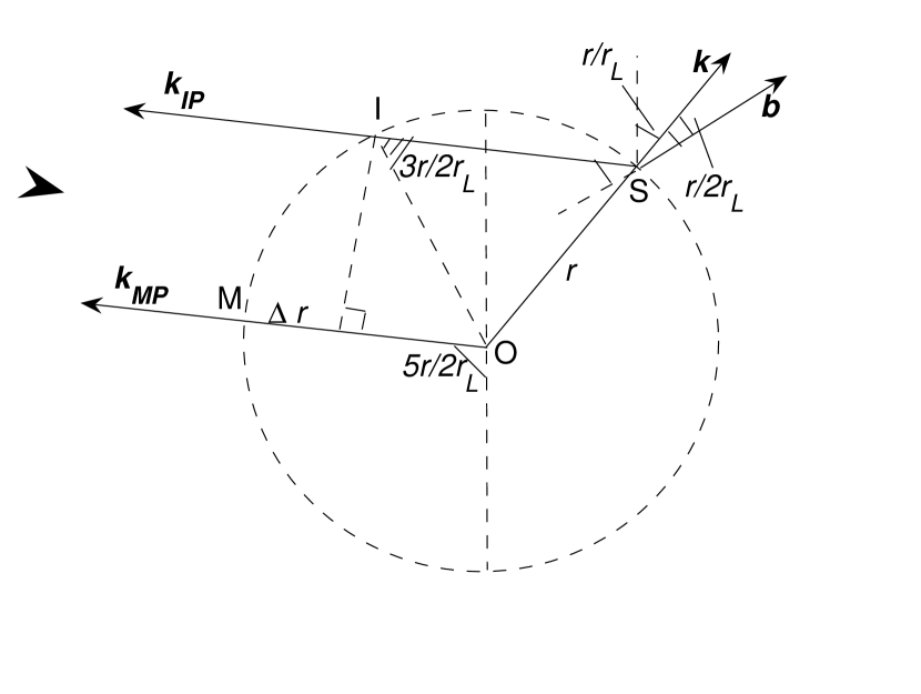
Figure 1: Geometrical scheme of the scattering in the transverse regime. The pulsar is assumed to be an orthogonal rotator with the rotational axis perpendicular to the plane of the figure and the magnetic axis rotating counterclockwise. For more details see the text.

Now let us consider the location of the scattered radiation in the pulse profile. For the sake of simplification it is assumed that the emission altitude is negligible as compared to the altitude of the scattering region, the ray geometry is dominated by the effect of magnetosphere rotation at the point of scattering, and the magnetic axis of a pulsar is perpendicular to the rotational axis. The scattered component resulting from the transverse scattering is antiparallel to the ambient magnetic field, and therefore is expected to be identified with the IP component in the pulse profile. The ray ${\bf k}$ emitted approximately along the magnetic axis at $t=0$ at the point O (see Fig. 1) comes to the point of scattering S at $t=r/c$, while the magnetic axis turns by the angle $\Omega r/c\equiv r/r_{L}$. The polar angle of the point of scattering with respect to the instantaneous magnetic axis is $r/r_{L}$, and in the dipolar geometry the angle between the ambient magnetic field vector ${\bf b}$ and the magnetic axis is $3r/2r_{L}$. Hence, the angle between ${\bf k}$ and ${\bf b}$ is $r/2r_{L}$. In the corotating frame, the wavevector of the scattered radiation, ${\bf k}_{s}^{(c)}$, is nearly antiparallel to ${\bf b}$, whereas in the laboratory frame it is shifted because of aberration by the angle $r/r_{L}$ in the direction of rotation. As can be seen from Fig. 1, the scattered ray ${\bf k}_{{\rm IP}}$ travels from the point of scattering to the point I for $\Delta t_{\rm IP}=2(r/c)\cos(3r/2r_{L})$ and later on reaches the observer. The main pulse is characterized by the parallel ray ${\bf k}_{\rm MP}$, which is emitted along the magnetic axis and points toward the observer. The ray ${\bf k}_{\rm MP}$ originates later than ${\bf k}$ by $\Delta t=\Delta\varphi/\Omega$, where $\Delta\varphi=\pi-3r/2r_{L}$ is the angle between the two instantaneous positions of the magnetic axis, and comes to the point M for the time $r/c$. Here it should be noted that the points I and M are equidistant from the point O, but not from the observer. The point I is located $\Delta r=r[1-\cos(3r/2r_{L})]$ farther, the distinction becoming significant at $r\sim r_{L}$. Taking into account that the difference in pulse longitude is related to the difference in arrival times as $\Delta\lambda=2\pi\Delta t/P$, we find finally that

$$\lambda_{\rm MP}-\lambda_{\rm IP}=\pi-\frac{5}{2}\frac{r}{r_{L}}-\frac{r}{r_{L}}\cos\left(\frac{3r}{2r_{L}}\right),$$

or, equivalently,

$$\lambda_{\rm IP}-\lambda_{\rm MP}=\pi+\frac{5}{2}\frac{r}{r_{L}}+\frac{r}{r_{L}}\cos\left(\frac{3r}{2r_{L}}\right).$$ (15)

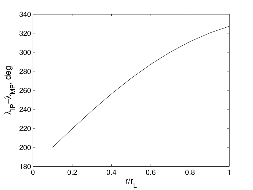
Figure 2: The IP location in the pulse profile as a function of altitude of the scattering region.

Thus, the IP lags the MP by more than $\pi$. Figure 2 shows the separation of the two components as a function of the height of the scattering region. For a number of pulsars, the IP positions in the pulse profile appear compatible with our model. At the same time, it is difficult to explain the cases when the IP lags the MP by less than $\pi$. Note that our geometrical examination is based solely on the effect of rotational aberration in the scattering region. A more realistic consideration including the magnetic field distortions close to the light cylinder and the propagation effects on the scattered radiation would possibly release the requirement of a nearly orthogonal rotator and allow the scattered component to lag the MP by less than $180^{\circ}$ to account for the postcursors in the pulsar profiles.

3 DISCUSSION

The induced Compton scattering of pulsar radio emission off the secondary plasma particles inside the open field line tube may play a significant role. The magnetic field of a pulsar affects the scattering process substantially. At distances of order of the emission altitude, the magnetic field is typically strong enough for the scattering to occur in the longitudinal regime, $\gamma^{2}\nu^{\prime^{4}}/\nu_{G}^{4}\ll 1$. Then the photons of the pulsar radio beam are predominantly scattered into the state with $\theta_{1_{\rm max}}\sim 1/\gamma$ and $\nu_{1}\sim\nu\theta^{2}\gamma^{2}\gg\nu$, i.e. the scattered radiation is almost aligned with the ambient magnetic field. As the magnetic field strength decreases with distance from the neutron star, at higher altitudes the longitudinal scattering regime changes for the transverse one, which holds on condition that $1/\gamma^{2}\ll\nu^{\prime^{4}}/\nu_{G}^{4}\ll 1$. In this regime, the orientations of the scattered photons are mostly antiparallel to the magnetic field, $\theta_{1_{\rm max}}=\pi$, and $\nu_{1}=\nu\theta^{2}/4\ll\nu$. The radiation scattered in the two regimes may from separate components in the pulse profile, which can be identified with the precursor and the IP. Apart from explaining the geometrical location of these components in the pulse profile, our model suggests the MP-IP and MP-precursor connections as well as can account for the peculiar properties of the emission components outside of the MP.

3.1 Comparison with Other Geometrical Models

In the geometrical aspect, our model is akin to the bidirectional model of Dyks et al. (2005). In that model, the precursor and IP originate at a certain location in the outer magnetosphere and the pulsar is approximately an orthogonal rotator. Because of the ultrarelativistic outstream of the plasma particles along the field lines, any conceivable emission mechanism would generate the outward radiation directed along the magnetic field in the corotating frame. The inward radiation is assumed to be antiparallel to the outward one. Thus, the orientations of the emission components and their locations in the pulse profile are roughly the same as in our model. Note, however, that in our case the precursor and the IP result from the scattering in the two distinct regimes and therefore originate at somewhat different altitudes. Besides that, the scattering sites are restricted to the region of the radio beam passage in the rotating magnetosphere. Correspondingly, the positions of the precursor and the IP in the pulse profile are tightly connected to that of the MP.

3.2 General Features of IPs

3.2.1 Spectral Behavior

As the scattered component arises in the outer magnetosphere, its position in the pulse profile is determined by the rotational aberration. The scattering region lies at distances of order of the cyclotron resonance radius, $r_{c}$, where $\nu\gamma\theta^{2}/2\equiv\nu_{G}$. Taking into account that $\omega_{G}\propto B\propto r^{-3}$ and $\theta\propto r$ one can see that $r_{c}$ is a weak function of radio frequency, $r_{c}\propto\nu^{-1/5}$, and hence the IP separation from the MP is almost the same over a wide frequency range. This is compatible with observations: as a rule, the IP position in the profile appears independent of frequency (e.g. Hankins & Fowler, 1986). Note that in the simplified case of orthogonal rotator and purely dipolar magnetic field considered in the present paper the rotational aberraion causes the IP to lag the MP by more than a half of the pulsar period. A more general treatment of the pulsar geometry including the peculiarities close to the light cylinder, is expected to account for smaller IP separations as well.

In the approximation considered, the induced scattering results in a net intensity transfer from the radio beam to the background, the total intensity of the two beams being constant. Hence, the maximum intensity of the scattered component, $I_{\nu_{1}}^{\max}(\nu_{1})$, is restricted to the original intensity of the radio beam, $I_{\nu}^{(0)}(\nu)$. Since the intensity is transferred to the lower frequency, $\nu_{1}=\nu\theta^{2}/4\ll\nu$, and the pulsar radiation has a decreasing spectrum, $I_{\nu_{1}}^{\rm max}(\nu_{1})$ may appear considerably less than the MP intensity at the same frequency. In a number of cases, the IPs are indeed much weaker than the MP. It should be noted, however, that at a fixed frequency the MP and IP may compete in intensity if the MP is noticeably suppressed by the scattering into still lower frequencies.

We have examined the scattering of radiation of a fixed frequency, but, generally speaking, it is a broadband process. Since the scattering efficiency $\Gamma_{\rm t}$ strongly depends on frequency, the scattering should affect the spectra of the MP and IP emissions. According to equation (12), at lower frequencies the scattering is more efficient and, although the intensity transfer approaches the stage of saturation, $\xi\gtrsim 1$, the growth of the IP component is believed to be noticeably stronger. This trend agrees with the observations, which testify that the IP phenomenon is most pronounced at the decameter wavelengths, at the edge of the observed radio frequency range (Bruck & Ustimenko, 1977, 1979; Bruck, 1987). Furthermore, the scattering can markedly suppress the MP emission at low frequencies, so that the MP spectrum may somewhat flatten. The IPs really have steeper spectra than the MPs, with the intensity ratio of the IP and MP markedly decreasing with frequency (e.g. Hankins & Fowler, 1986).

3.2.2 Statistics of Pulsars with IPs

The estimate of the scattering efficiency (12) implies that the intensity transfer is more significant at larger radio luminosities, shorter periods, and weaker magnetic field strengths. The IPs are indeed met in the pulsars with periods $P\lesssim 0.6$ s (Manchester & Lyne, 1977). Moreover, the population of normal short-period pulsars, $P\sim 0.1$ s, is generally characterized by larger radio luminosities than that of the long-period ones. As for the millisecond pulsars, their luminosities are somewhat less (Kramer et al., 1998), but very short periods, $P\sim 1-10$ ms, and weak magnetic fields, $B_{\star}\sim 10^{8}-10^{9}$ G, favor even larger scattering efficiencies. Note that the pulsars with IPs are indeed more abundant in the population of the millisecond pulsars.

3.2.3 Polarization Properties

Our model of IP formation as a result of induced scattering of the MP implies peculiar polarization properties of the scattered component. In contrast to the longitudinal scattering, when the intensity may be efficiently transferred only between the photon states with the ordinary polarization and the scattered component is characterized by the complete linear polarization, the transverse scattering involves both orthogonal polarizations and the situation is more complicated. For different channels of the scattering, the efficiency of intensity transfer differs by the factor $g^{ij}$, which is generally of order unity. In case of intense scattering (see eq.[8]), the difference in $g^{ij}$ and $I_{\nu}^{(0)}$ for various channels may play a significant role, and the intensity transfer in one of the channels may substantially dominate that in the others, so that the scattered component may be strongly polarized. Note that the observed IPs are typically characterized by higher percentage of linear polarization than the MPs (e.g. Rankin & Rathnasree, 1997; Weltevrede et al., 2007), with the giant IPs showing almost complete linear polarization (Eilek & Hankins, 2007).

Our model also suggests a specific behavior of the position angle of linear polarization in the IP emission. The position angle of the scattered radiation is determined by the orientation of the ${\bf k_{1}}\times{\bf b}$-plane in the scattering region and therefore should somewhat differ from that of the MP. Besides that, the MP and IP may be dominated by different polarization modes, in which case the position angle of the IP is additionally shifted by $90^{\circ}$. As the scattering region lies in the outer magnetosphere, in the area covered by the radio beam the magnetic field is almost uniform and hence the position angle should remain practically unchanged across the IP. All this is in line with the observational data (e.g. Rankin & Rathnasree, 1997; Moffett & Hankins, 1998; Weltevrede et al., 2007).

3.3 Intensity Modulation at Different Timescales

As is discussed above, the origin of IPs as a result of the MP scattering far from the emission region can account for a number of distinctions in the properties of the MP and IP emissions. At the same time, our model implies a physical connection between these emissions, which is believed to manifest itself as a correlation of the temporal fluctuations of the MP and IP and also as a consistency of the angular and frequency structures in the two components. The idea of the MP-IP connection is strongly supported by a number of observational results.

3.3.1 Subpulse Modulation

Recent observations of PSR B1702-19 (Weltevrede et al., 2007) have shown that the subpulse pattern in the IP is characterized by exactly the same periodicities as that in the MP. Moreover, the intensity fluctuations appear correlated with a delay of about a half of the pulsar period. This is just what can be expected if the MP is partially scattered into the IP. As the subpulse pattern is independent of frequency, the subpulse modulation in the scattered component should repeat that in the incident radiation. The MP and the IP seen by an observer originate at different phases of pulsar rotation, and therefore they should arise at different phases of subpulse drift and the intensities should be correlated with a certain temporal delay. It is worth noting that this delay should not exactly correspond to the longitudinal separation between the MP and IP in the profile, since the components travel somewhat different distances to the observer.

3.3.2 Microstructure

The microstructure characteristic of the MP emission is also expected to be present in the scattered component. The observations of PSR B0950+08 have indeed revealed the microstructure in the IP at the timescale $\tau_{\rm IP}=90\,\mu$s, whereas in the MP $\tau_{\rm MP}=130\,\mu$s (Hankins & Cordes, 1981; Hankins & Boriakoff, 1981). In our model, the relationship between the microstructure timescales in the two components can be estimated as follows. The intensity is transferred between the photon states related as $\nu(1-\beta\cos\theta)=\nu_{1}(1-\beta\cos\theta_{1})$. Differentiating this at fixed frequencies yields $\nu\theta\Delta\theta=\nu_{1}\Delta\theta^{2}$, where it is taken that $\sin\theta_{1}\approx\Delta\theta_{1}$ for $\theta_{1}\approx\pi$. As $\tau_{\rm IP}/\tau_{\rm MP}=\Delta\theta_{1}/\Delta\theta$ and $\nu\theta^{2}/2\approx 2\nu_{1}$, one can find that $\tau_{\rm IP}(\nu_{1})/\tau_{\rm MP}(\nu)=2/\sqrt{\theta\Delta\theta}$. Taking into account that the microstructure timescale evolves with frequency, $\tau_{\rm MP}\propto\nu^{-\alpha}$, we obtain finally:

$$\frac{\tau_{\rm IP}(\nu_{1})}{\tau_{\rm MP}(\nu_{1})}=\frac{2(\theta^{2}/4)^{\alpha/2}}{\sqrt{\theta\Delta\theta(\nu_{1})}}.$$ (16)

In case of PSR B0950+08, $P=0.25$ s and $\tau_{\rm MP}=130\,\mu$s, so that the angular scale of microstructure $\Delta\theta=2\pi\tau/P\sim 3\cdot 10^{-3}$. Then with $\theta=0.2$ and $\alpha=2$ we have $\tau_{\rm IP}/\tau_{\rm MP}=0.8$, which is consistent with the observed value of about 0.7. Thus, our model can account for the difference in the microstructure timescales of the MP and the IP.

3.3.3 Giant IPs in the Crab Pulsar

Recent observations of the MP and IP of the Crab pulsar (Eilek & Hankins, 2007) have revealed quite distinct temporal and frequency structures of the giant pulses in these components. The giant MPs generally present one or several broadband microbursts, which consist of narrowband ($\delta\nu/\nu\sim 0.1$) nanoshots of a duration $\delta t\sim 10/\nu\sim 10^{-8}-10^{-9}$ s. The giant IPs consist of the proportionally spaced narrow emission bands of microsecond lengths organized into several band sets, which appear at somewhat different times and exhibit a marked drift toward higher frequencies. Below we examine the modification of the temporal and frequency structure of the giant MPs as a result of induced scattering into the background and argue that the consequent structure of the scattered component is compatible with that really seen in the giant IPs.

Since the intensity is transferred between the frequencies approximately related as $\nu\theta^{2}/2=\widetilde{\nu}/\gamma^{2}=2\nu_{1}$, the frequency structure of the IP at a fixed pulse longitude can be derived from differentiating this equation: $\Delta\nu\theta^{2}/2+\nu\theta\Delta\theta=2\Delta\nu_{1}$. As the nanoshot width is extremely small, $\delta\theta=2\pi\delta t/P\sim 10^{-6}-10^{-7}$ (here the period of the Crab pulsar $P=0.03$ s), the main contribution to $\Delta\nu_{1}$ comes from the first term, and we have

$$\frac{\Delta\nu_{1}}{\nu_{1}}\sim\frac{\Delta\nu}{\nu}\sim 0.1.$$ (17)

Thus, the proportionally spaced emission bands of the IP(with $\delta\nu_{1}/\nu_{1}\approx 0.06$) can naturally be attributed to the modification of the nanoshot bandwidths as a result of induced scattering.

The temporal durations of the bands in the IP can be estimated by means of equation (16). Note that because of the extremely short durations of the original nanoshots, the scattered nanoshots are noticeably enlarged: $\tau_{\rm IP}\propto\Delta\theta^{-1/2}$. For $\alpha=2$, $\theta=0.5$ and $\tau_{\rm MP}(\nu_{1})\sim 10^{-8}-10^{-9}$ s we have $\tau_{\rm IP}\sim 0.4-1.2\,\mu$s, which agrees with the observational data. Keeping in mind that $\nu\theta^{2}/2=2\nu_{1}$, one can see that at a given frequency $\nu$ different parts of the nanoshot and the neighboring nanoshots are scattered to somewhat different $\nu_{1}$, leading to a slight drift of the scattered bands toward higher frequencies, just as is really observed. Thus, the peculiar temporal and frequency structure of the giant IPs can indeed be explained in terms of induced scattering of the giant MPs.

3.3.4 Mode Changes in PSR B1822-09

The pulsar B1822-09 is known to exhibit a peculiar mode changing behavior: In the bright mode, its profile contains a strong precursor and a weak IP, whereas in the weak mode the IP is strong and the precursor is almost absent (Fowler et al., 1981; Fowler & Wright, 1982; Gil et al., 1994). Within the framework of our model, this can be interpreted as a competition between the processes of induced scattering of the MP in the longitudinal and transverse regimes. The variations of the scattering efficiencies can naturally be attributed to the fluctuations of the number density of the scattering particles. Furthermore, the fluctuations of the plasma number density lead to changes in the emission altitude of the MP radiation, which may affect the applicability of the longitudinal scattering regime.

Larger multiplicities of the plasma, $\kappa$, imply larger emission altitudes for a given frequency, in which case the gyrofrequency appears low enough to preclude the longitudinal scattering even in the vicinity of the emission region. At the same time, larger $\kappa$ favor stronger transverse scattering. As a result, the precursor component is not formed, whereas the intensity transfer to the IP is so efficient that the MP is markedly suppressed. As the intensity is transferred from higher to lower frequencies, $\nu_{1}=\nu\theta^{2}/4$, and the radio beam originally has a decreasing spectrum, the IP remains weak as compared to the MP at the same frequency. Thus, the weak mode is characterized by larger plasma multiplicities and, correspondingly, by an efficient intensity transfer from higher to lower frequencies, in which case the total intensity of the pulse profile markedly decreases.

In the bright mode, the plasma number density is smaller, the emission altitude lower, and the longitudinal scattering holds in addition to the transverse one. The longitudinal scattering gives rise to the precursor in the pulse profile, whereas the transverse scattering, being less efficient because of lower $\kappa$, forms a weaker IP. As is evident from equation (14), the transverse scattering may be much more efficient in taking the intensity from the MP at a given frequency. At the same time, if one compare the intensity growth of the precursor and the IP at a given frequency, it is necessary to keep in mind that these components are fed by the MP intensity at substantially different frequencies, $\nu_{1}^{(\rm Pr)}=\nu\theta^{2}\gamma^{2}\gg\nu$ and $\nu_{1}^{(\rm IP)}=\nu\theta^{2}/4\ll\nu$. With the decreasing spectrum of pulsar radiation, this implies much larger $\Gamma_{\rm l}/\Gamma_{\rm t}$ than that given by equation (14), so that both scattering efficiencies can be concurrently substantial. Since the longitudinal scattering transfers the intensity to the precursor from much lower frequencies, this component may be strong enough as compared to the MP at the same frequency. Note that the precursor in the profile of PSR B1822-09 is really comparable in intensity to the MP and is much stronger than the IP, providing a strong support to our scenario of intensity transfer between widely spaced frequencies in the course of induced scattering of the MP into the background.

4 CONCLUSIONS

We have considered the induced Compton scattering of radio emission by the particles of the hot magnetized electron-positron plasma, which streams along the open field lines of the pulsar magnetosphere. In the presence of a strong magnetic field, $\nu^{\prime}\ll\nu_{G}$, two scattering regimes are possible, the longitudinal and transverse ones, both being relevant to the pulsar case. The earlier studies of the magnetized induced scattering in pulsars were typically restricted to the longitudinal regime. In the present paper, we have generalized the kinetic equation to include the transverse scattering regime as well and have used it to solve the problem on the transverse induced scattering of the radio beam into the background.

Our problem can be reduced to examining the scattering between the two photon states, one of which represents the radio beam, whereas another one is the background state corresponding to the maximum scattering probability for the beam photons. Since in the particle rest frame the photon frequency is almost unchanged in the scattering act, in the laboratory frame the photon states interacting via induced scattering obey the condition $\nu(1-\beta\cos\theta)=\nu_{1}(1-\beta\cos\theta_{1})$. In contrast to the longitudinal regime, in which case the radio beam photons are predominantly scattered into the direction nearly along the ambient magnetic field ($\theta_{1_{\rm max}}\sim 1/\gamma$ and $\nu_{1}\sim\nu\theta^{2}\gamma^{2}\gg\nu$), the photons scattered in the transverse regime are mostly antiparallel to the field ($\theta_{1_{\rm max}}\approx\pi$ and $\nu_{1}\sim\nu\theta_{1}^{2}\ll\nu$). In both regimes, the induced scattering results in the intensity redistribution between the two photon states, with the total intensity remaining approximately unchanged. This specific character of intensity evolution is determined by the role of the magnetic field in the scattering process and differs substantially from the non-magnetic case, when the scattering results in the photon drift toward lower frequencies.

The magnetized induced scattering of the radio beam into the background, which takes place in the open field line tube of a pulsar, is suggested to underlie the formation of additional components in the pulse profile outside of the MP. Given that the pulsar is a nearly orthogonal rotator, the longitudinal scattering gives rise to the precursor component located a few tens degrees ahead of the MP, whereas the transverse scattering forms the IP, which lags the MP by more than $180^{\circ}$. The numerical estimates show that at the conditions relevant to pulsar magnetospheres the intensity transfer from the radio beam to the background can indeed be efficient. Stronger scattering is favored by shorter pulse periods, larger radio luminosities and lower frequencies and is expected to be especially efficient in the millisecond pulsars. All this is in line with the trends known for the observed IP emission. Note that the IP component is fed by the MP radiation of much higher frequencies, $\nu_{1}\approx\nu\theta^{2}/4$. With the decreasing spectrum of the original MP, this implies that the IP cannot be as large as the MP at the same frequency unless the latter is substantially suppressed by the scattering to still lower frequencies.

Our model can account for the peculiar properties of the IP emission. As the region of efficient transverse scattering lies far from the emission region, at distances of order of the cyclotron resonance radius, and the characteristic scattering altitude is an extremely weak function of frequency, the MP-IP separation should remain almost the same over the observed radio frequency range. Note that the scattering at somewhat lower altitudes may also be noticeable, giving rise to the emission bridge between the MP and the IP.

The position angle of linear polarization of the scattered radiation is determined by the orientation of the ${\bf k_{1}}\times{\bf b}$-plane in the scattering region and generally differs from the position angle of the incident radiation. Furthermore, the magnetic field is believed to be almost uniform throughout the scattering region, so that the position angle swing in the IP should be shallow. Although both orthogonal polarization modes can grow as a result of the transverse scattering, the efficiencies of intensity transfer may differ markedly, making expect high percentage of linear polarization in the resultant IP emission.

The IP formation as a result of the MP scattering implies a physical connection between these components, which is believed to manifest itself in their intensity fluctuations at different timescales. Our model is strongly supported by the recent observations of PSR B1702-19 (Weltevrede et al., 2007), which have revealed that the subpulse patterns in the MP and the IP are intrinsically in phase. Furthermore, the peculiar temporal and frequency structure of the giant pulses in the IP of the Crab pulsar (Eilek & Hankins, 2007) may well be interpreted as a modification of the giant MP structure in the scattering process. The peculiar moding behavior of PSR B1822-09 is suggested to result from the fluctuations of the physical conditions in the scattering region, which affect the relative efficiency of the longitudinal and transverse scatterings and lead to the observed interplay between the resultant precursor and IP components.

The pulse-to-pulse fluctuations of the plasma number density and the original MP intensity, which affect the scattering efficiency, are believed to result in the peculiar intensity statistics of the IP. Moreover, in some pulsars this component may be seen only occasionally. Note that the transient IPs are difficult to detect and they are yet to be found observationally, though some evidence for occasional strong events at the IP longitudes is already known (Hankins & Cordes, 1981; Biggs, 1990). Despite the relative weakness of the IPs in most of the known cases, the present progress in the observational facilities seems to promise an opportunity of the comprehensive study of the IP emission at a single-pulse level.

In the present paper, we for the first time suggest a physical model of the IP formation. It is believed to stimulate further observational investigations aimed at revealing the peculiar properties of the IP emission and the manifestations of its connection to the MP.

Appendix A BASIC FORMALISM OF THE MAGNETIZED INDUCED SCATTERING

Following Blandford & Scharlemann (1976); Petrova (2007), let us consider the induced scattering in the laboratory frame between the two photon states, $\bf k$ and ${\bf k_{1}}$, involving the electrons with the initial momenta $p$ and $p+\delta p$. The electrons are confined to move along the magnetic field line, and in the scattering act the momentum parallel to the field is conserved, so that

$$\delta p=\hbar k\cos\theta-\hbar k_{1}\cos\theta_{1},$$ (A1)

where $\theta$ and $\theta_{1}$ are the wavevector tilts to the magnetic field for the photons in the states $\bf k$ and $\bf k_{1}$. The rate of change of the photon occupation number as a result of induced scattering is

$$\frac{{\rm d}n}{{\rm d}t}\frac{{\rm d}^{3}\bf k}{(2\pi)^{3}}=\int[f(p+\delta p)-f(p)]\frac{{\rm d}P}{{\rm d}t}n_{1}{\rm d}p.$$ (A2)

Here $n$ and $n_{1}$ are the photon occupation numbers in the states $\bf k$ and $\bf k_{1}$, respectively, $f(p)$ is the electron distribution function, ${\rm d}P/{\rm d}t$ is the probability of generating spontaneously scattered photons per electron per unit time,

$$\frac{{\rm d}P}{{\rm d}t}=n\frac{\rm d^{3}{\bf k}}{(2\pi^{3})}\eta\frac{{\rm d}\sigma}{{\rm d}\Omega_{1}}c^{4}\frac{{\rm d}^{3}\bf k_{1}}{\omega_{1}^{2}}\delta\left(\omega_{1}-\eta\omega/\eta_{1}\right),$$ (A3)

where $\eta\equiv 1-\beta\cos\theta$, $\eta_{1}\equiv 1-\beta\cos\theta_{1}$, ${\rm d}\sigma/{\rm d}\Omega_{1}$ is the scattering cross-section per unit solid angle, and the argument of the delta-function means that in the particle rest frame the initial and final frequencies are equal, $\omega\gamma\eta\equiv\omega_{1}\gamma\eta_{1}$. We assume that the photon occupation numbers change only because of the photon propagation through the stationary flow, so that ${\rm d}n/{\rm d}t=c{\rm d}n/{\rm d}r$. Taking into account that $f(p+\delta p)-f(p)\approx\delta p(\partial f/\partial p)$, we integrate equation (A2) by parts, substitute equations (A1) and (A3) and integrate this over $k_{1}$ with the help of delta-function to obtain

$$\frac{{\rm d}n}{{\rm d}r}=\int{\rm d}\gamma F\frac{\beta\hbar\omega}{mc^{2}}\int(\cos\theta_{1}-\cos\theta)\frac{\partial}{\partial\gamma}\left[nn_{1}\frac{{\rm d}\sigma}{{\rm d}\Omega_{1}}\right]{\rm d}\Omega_{1}.$$ (A4)

Here $F(\gamma)$ stands for the distribution function in Lorentz-factor.

The above kinetic equation describes the photon transfer as a result of induced scattering in a hot magnetized plasma. We consider the scattering of the ordinary and extraordinary transverse electromagnetic waves. Their polarization states, with the electric vectors in the plane of the wavevector and the ambient magnetic field and orthogonal to this plane, are designated as A- and B-polarizations, respectively. The classical scattering cross-section in an arbitrary magnetic field has been derived by Canuto et al. (1971). Expanding their result in a power series of $\omega^{\prime 2}/\omega_{G}^{2}$ and retaining the first two terms yield

$$\frac{{\rm d}\sigma^{AA}}{{\rm d}\Omega_{1}^{\prime}}\approx r_{e}^{2}\sin^{2}\theta^{\prime}\sin^{2}\theta_{1}^{\prime}+r_{e}^{2}\frac{\omega^{\prime 2}}{\omega_{G}^{2}}\left\{\cos^{2}\theta^{\prime}\cos^{2}\theta_{1}^{\prime}\left[\sin^{2}\Delta\phi^{\prime}+\frac{\omega^{\prime 2}}{\omega_{G}^{2}}(1+\sin^{2}\Delta\phi^{\prime})\right]\right.$$

$$\left.-\frac{1}{2}\left(1+\frac{\omega^{\prime 2}}{\omega_{G}^{2}}\right)\sin 2\theta^{\prime}\sin 2\theta_{1}^{\prime}\cos\Delta\phi^{\prime}\right\}.$$ (A5a)

$$\frac{{\rm d}\sigma^{BA}}{{\rm d}\Omega_{1}^{\prime}}\approx r_{e}^{2}\frac{\omega^{\prime 2}}{\omega_{G}^{2}}\cos^{2}\theta_{1}^{\prime}\left[\cos^{2}\Delta\phi^{\prime}+\frac{\omega^{\prime 2}}{\omega_{G}^{2}}(1+\cos^{2}\Delta\phi^{\prime})\right],$$ (A5b)

$$\frac{{\rm d}\sigma^{AB}}{{\rm d}\Omega_{1}^{\prime}}\approx r_{e}^{2}\frac{\omega^{\prime 2}}{\omega_{G}^{2}}\cos^{2}\theta^{\prime}\left[\cos^{2}\Delta\phi^{\prime}+\frac{\omega^{\prime 2}}{\omega_{G}^{2}}(1+\cos^{2}\Delta\phi^{\prime})\right].$$ (A5c)

$$\frac{{\rm d}\sigma^{BB}}{{\rm d}\Omega_{1}^{\prime}}\approx r_{e}^{2}\frac{\omega^{\prime 2}}{\omega_{G}^{2}}\left\{\sin^{2}\Delta\phi^{\prime}+\frac{\omega^{\prime 2}}{\omega_{G}^{2}}[1+\sin^{2}\Delta\phi^{\prime}]\right\}.$$ (A5d)

Here the superscripts of $\sigma$ denote the initial and final polarization states of a photon, the primes mark the quantities in the electron rest frame, $r_{e}$ is the classical electron radius, $\Delta\phi^{\prime}=\phi^{\prime}-\phi_{1}^{\prime}$, $(\theta^{\prime},\phi^{\prime})$ and $(\theta_{1}^{\prime},\phi_{1}^{\prime})$ are the spherical angles of the initial and final photon wavevectors ${\bf k^{\prime}}$ and $\bf k_{1}^{\prime}$ in the coordinate system with the polar axis along the magnetic field, and $\omega^{\prime}=\omega_{1}^{\prime}$.

Using relativistic transformations,

$$\omega^{\prime}=\omega\gamma\eta,\quad\Delta\phi^{\prime}=\Delta\phi,\quad{\rm d}\Omega_{1}^{\prime}=\frac{{\rm d}\Omega_{1}}{\gamma^{2}\eta_{1}^{2}},\quad\cos\theta^{\prime}=\frac{\cos\theta-\beta}{1-\beta\cos\theta},\quad\sin\theta^{\prime}=\frac{\sin\theta}{\gamma\eta},$$ (A6)

one can express the cross-sections in terms of the quantities of the laboratory frame, substitute this into equation (A4) and perform differentiation with respect to $\gamma$. It should be noted that the dominant term of the cross-sections, $\propto\omega^{\prime^{2}}/\omega_{G}^{2}$ as well as the remaining factor in the expression under differentiation in equation (A4) depend on $\gamma$ only implicitly, via $\eta(\beta)$ and $\eta_{1}(\beta)$, which are weak functions of $\gamma$: ${\rm d}\beta/{\rm d}\gamma=1/\beta\gamma^{3}\ll 1/\gamma$. Therefore it is necessary to retain the second-order terms, $\propto\omega^{\prime^{4}}/\omega_{G}^{4}$, which introduce the explicit dependence on $\gamma$. Although they are small, their derivatives may contribute significantly. Keeping in mind these considerations, one can obtain the kinetic equations in the following form:

$$\frac{{\rm d}n}{{\rm d}r}(A\to A)=\frac{\hbar nr_{e}^{2}}{mc}\int{\rm d}\gamma F\int\frac{\sin^{2}\theta\sin^{2}\theta_{1}}{\gamma^{6}\eta^{3}\eta_{1}^{3}}\left\{\frac{(\eta-\eta_{1})^{2}}{\beta^{2}\gamma^{3}\eta_{1}^{2}}\frac{\partial n_{1}k_{1}^{2}}{\partial k_{1}}\right.$$

$$\left.+\frac{6(\eta_{1}-\eta)n_{1}k\eta^{2}}{\beta^{2}\gamma\eta_{1}^{2}}\left[1-\frac{\eta+\eta_{1}}{2\gamma^{2}\eta\eta_{1}}\right]\right\}{\rm d}\Omega_{1}$$

$$+\frac{\hbar nr_{e}^{2}}{mc}\int{\rm d}\gamma F\int\frac{\omega^{2}}{\omega_{G}^{2}}\sin^{2}\Delta\phi\left\{\frac{(\eta-\eta_{1})^{2}}{\beta^{2}\gamma^{3}\eta_{1}^{2}}\frac{1}{k}\frac{\partial n_{1}k_{1}^{3}}{\partial k_{1}}\frac{(1-\eta\gamma^{2})^{2}}{\beta^{2}\gamma^{4}\eta^{2}}\frac{(1-\eta_{1}\gamma^{2})^{2}}{\beta^{2}\gamma^{4}\eta_{1}^{2}}\right.$$

$$\left.+\frac{2(\eta-\eta_{1})kn_{1}\eta^{3}}{\beta^{6}\gamma^{11}\eta_{1}^{3}}\left[\frac{(\eta\gamma^{2}-1)[\eta\gamma^{2}(2-\eta)-1]}{\eta^{3}}\frac{(1-\eta_{1}\gamma^{2})^{2}}{\eta_{1}^{2}}\right.\right.$$

$$\left.\left.+\frac{(\eta_{1}\gamma^{2}-1)[\eta_{1}\gamma^{2}(2-\eta_{1})-1]}{\eta_{1}^{3}}\frac{(1-\eta\gamma^{2})^{2}}{\eta^{2}}\right]\right\}{\rm d}\Omega_{1}$$

$$-\frac{\hbar nr_{e}^{2}}{mc}\int{\rm d}\gamma F\int\frac{\omega^{2}}{\omega_{G}^{2}}\frac{\cos\Delta\phi\sin 2\theta\sin 2\theta_{1}}{\mu\mu_{1}\beta^{2}\gamma^{3}}\left\{\frac{(\eta-\eta_{1})^{2}}{2\gamma^{2}\eta_{1}^{2}}\frac{1}{k}\frac{\partial n_{1}k_{1}^{3}}{\partial k_{1}}\right.$$

$$\left.-\frac{(\eta-\eta_{1})kn_{1}\eta^{3}}{\eta_{1}^{3}}\left[1-\frac{\mu+\mu_{1}}{2\gamma^{2}\mu\mu_{1}}\right]\right\}{\rm d}\Omega_{1}$$

$$+\frac{\hbar nr_{e}^{2}}{mc}\int{\rm d}\gamma F\int\frac{\omega^{4}}{\omega_{G}^{4}}\frac{(\eta-\eta_{1})n_{1}k\eta^{4}(\eta\gamma^{2}-1)}{\eta_{1}^{3}\beta^{2}\gamma}\left[2(1+\sin^{2}\Delta\phi)\frac{(1-\eta\gamma^{2})^{2}}{\beta^{2}\gamma^{4}\eta^{2}}\frac{(1-\eta_{1}\gamma^{2})^{2}}{\beta^{2}\gamma^{4}\eta_{1}^{2}}\right.$$

$$\left.-\cos\Delta\phi\sin 2\theta\sin 2\theta_{1}\right]{\rm d}\Omega_{1}.$$ (A7a)

$$\frac{{\rm d}n}{{\rm d}r}(B\to A)=\frac{\hbar nr_{e}^{2}}{mc}\int{\rm d}\gamma F\int\frac{\omega^{2}}{\omega_{G}^{2}}\cos^{2}\Delta\phi\left\{\frac{(\eta-\eta_{1})^{2}}{\beta^{2}\gamma^{3}\eta_{1}^{2}}\frac{1}{k}\frac{\partial n_{1}k_{1}^{3}}{\partial k_{1}}\frac{(1-\eta_{1}\gamma^{2})^{2}}{\beta^{2}\gamma^{4}\eta_{1}^{2}}\right.$$

$$\left.+\frac{(\eta-\eta_{1})kn_{1}\eta^{3}}{\eta_{1}^{3}}\frac{2(\eta_{1}\gamma^{2}-1)}{\beta^{4}\gamma^{7}\eta_{1}^{3}}[\eta_{1}\gamma^{2}(2-\eta_{1})-1]\right\}{\rm d}\Omega_{1}$$

$$+\frac{2\hbar nr_{e}^{2}}{mc}\int{\rm d}\gamma F\int\frac{\omega^{4}}{\omega_{G}^{4}}(1+\cos^{2}\Delta\phi)\frac{(1-\eta_{1}\gamma^{2})^{2}}{\beta^{2}\gamma^{4}\eta_{1}^{2}}\frac{(\eta-\eta_{1})n_{1}k\eta^{4}(\eta\gamma^{2}-1)}{\eta_{1}^{3}\beta^{2}\gamma}{\rm d}\Omega_{1},$$ (A7b)

$$\frac{{\rm d}n}{{\rm d}r}(A\to B)=\frac{\hbar nr_{e}^{2}}{mc}\int{\rm d}\gamma F\int\frac{\omega^{2}}{\omega_{G}^{2}}\cos^{2}\Delta\phi\left\{\frac{(\eta-\eta_{1})^{2}}{\beta^{2}\gamma^{3}\eta_{1}^{2}}\frac{1}{k}\frac{\partial n_{1}k_{1}^{3}}{\partial k_{1}}\frac{(1-\eta\gamma^{2})^{2}}{\beta^{2}\gamma^{4}\eta^{2}}\right.$$

$$\left.+\frac{(\eta-\eta_{1})kn_{1}\eta^{3}}{\eta_{1}^{3}}\frac{2(\eta\gamma^{2}-1)}{\beta^{4}\gamma^{7}\eta^{3}}[\eta\gamma^{2}(2-\eta)-1]\right\}{\rm d}\Omega_{1}$$

$$+\frac{2\hbar nr_{e}^{2}}{mc}\int{\rm d}\gamma F\int\frac{\omega^{4}}{\omega_{G}^{4}}(1+\cos^{2}\Delta\phi)\frac{(1-\eta\gamma^{2})^{2}}{\beta^{2}\gamma^{4}\eta^{2}}\frac{(\eta-\eta_{1})n_{1}k\eta^{4}(\eta\gamma^{2}-1)}{\eta_{1}^{3}\beta^{2}\gamma}{\rm d}\Omega_{1}.$$ (A7c)

$$\frac{{\rm d}n}{{\rm d}r}(B\to B)=\frac{\hbar nr_{e}^{2}}{mc}\int{\rm d}\gamma F\int\frac{\omega^{2}}{\omega_{G}^{2}}\sin^{2}\Delta\phi\frac{(\eta_{1}-\eta)^{2}}{\eta_{1}^{2}\beta^{2}\gamma^{3}}\frac{1}{k}\frac{\partial n_{1}k_{1}^{3}}{\partial k_{1}}{\rm d}\Omega_{1}$$

$$+\frac{2\hbar nr_{e}^{2}}{mc}\int{\rm d}\gamma F\int\frac{\omega^{4}}{\omega_{G}^{4}}(1+\sin^{2}\Delta\phi)\frac{\eta\gamma^{2}-1}{\beta^{2}\gamma}\frac{\eta-\eta_{1}}{\eta_{1}^{3}}\eta^{4}n_{1}k{\rm d}\Omega_{1}.$$ (A7d)

The first term of the kinetic equation (A7d) is determined by the photon spectrum and is qualitatively similar to the right-hand side of the kinetic equation for the non-magnetic case (cf., e.g., eq.[2.13] in Lyubarskii & Petrova (1996)), signifying the monotonic shift of the photon distribution toward lower frequencies in the course of the scattering. The second term means the redistribution of photons between the states which satisfy the condition $\omega\eta\equiv\omega_{1}\eta_{1}$. Because of the factor $\eta-\eta_{1}$, the photon occupation numbers decrease as a result of the photon transfer to the states with $\theta_{1}>\theta$ and increase on account of the photons coming from the states with $\theta_{1}<\theta$. One can find that the ratio of the second term in equation (A7d) to the first one is $\sim\omega^{2}\eta^{2}\gamma^{2}/(\omega_{G}^{2})\chi^{2}\gamma^{2}$, where $\chi\equiv\min(\theta,\theta_{1})$. Thus, in the case of interest, in a moderately strong magnetic field, the second term dominates. Although the kinetic equations (A7b) and (A7c) are somewhat more complicated, their second terms also dominate on the same condition.

The equation (A7a) is worthy to be analyzed in more detail. Its first term, corresponding to the first term of the cross-section (A5a), does not contain the gyrofrequency and describes the longitudinal scattering, which remains efficient at $B\to\infty$. The second item of this term differs from the first one by the factor $(\theta_{1}\gamma)^{2}$ and hence dominates at $\theta_{1}\gg 1/\gamma$. In the regime of transverse scattering, $\chi^{2}\gamma^{2}\omega^{\prime 2}/\omega_{G}^{2}\gg 1$, the last term of equation (A7a) dominates, being at least a factor of $\chi^{4}\gamma^{4}\omega^{\prime 4}/\omega_{G}^{4}$ larger than the first one and $\chi^{2}\gamma^{2}\omega^{\prime 2}/\omega_{G}^{2}$ larger than the second and the third ones. The sign of the integrand in the last term is determined by that of $(\eta-\eta_{1})$, that is the photons are transferred to the states with $\theta_{1}>\theta$. This is similar to the corresponding terms in the kinetic equations (A7b), (A7c), and (A7d) and contrasts with the longitudinal regime, in which case the photons are transferred closer to the magnetic field direction, $\theta_{1}<\theta$ (cf. the second item in the braces of the first term in equation (A7a); for more details see Petrova (2007)).

References

- Biggs (1990) Biggs, J. D. 1990, MNRAS, 246, 341
- Blandford & Scharlemann (1976) Blandford, R. D., & Sharlemann, E. T. 1976, MNRAS, 174, 59
- Börner & Mészáros (1979) Börner, & Mészáros, P. 1979, A&A, 77, 178
- Bruck & Ustimenko (1977) Bruck, Yu. M., & Ustimenko, B. Yu. 1977, Ap&SS, 49, 349
- Bruck & Ustimenko (1979) Bruck, Yu. M., & Ustimenko, B. Yu. 1979, A&A, 80, 170
- Bruck (1987) Bruck, Yu. M. 1987, Aust. J. Phys., 40, 861
- Canuto (1970) Canuto, V. 1970, ApJ, 160, 153
- Canuto et al. (1971) Canuto, V., Lodenquai, J., & Ruderman, M. 1971, Phys. Rev. D, 3, 2303
- Chou (1986) Chou, C. K. 1986, Ap&SS, 121, 333
- Cordes et al. (2004) Cordes, J. M., Bhat, N. D. R., Hankins, T. H., McLaughlin, M. A., & Kern, J. 2004, ApJ, 612, 375
- Dyks et al. (2005) Dyks, J., Zhang, B., & Gil, J. 2005, ApJ, 626, L45
- Eilek & Hankins (2007) Eilek, J. A., & Hankins, T. H. 2007, in Proceedings of the 363. WE-Heraeus Seminar: Neutron Stars and Pulsars (Posters and contributed talks) Physikzentrum Bad Honnef, Germany, May.14-19, 2006, eds. W.Becker, H.H.Huang, MPE Report 291, p.112
- Fowler et al. (1981) Fowler, L. A., Wright, G. A. E., & Morris, D. 1981, A&A, 93, 54
- Fowler & Wright (1982) Fowler, L. A., & Wright, G. A. E. 1982, A&A, 109, 279
- Gangadhara & Krishan (1993) Gangadhara, R. T., & Krishan, V. 1993, ApJ, 415, 505
- Gil (1985) Gil, J. 1985, ApJ, 299,154
- Gil et al. (1994) Gil, J. A. et al. 1994, A&A, 282, 45
- Hamada & Kanno (1974) Hamada, T., & Kanno, S. 1974, PASJ, 26,421
- Hankins & Cordes (1981) Hankins, T. H., & Cordes, J. M. 1981, ApJ, 249, 241
- Hankins & Boriakoff (1981) Hankins, T. H., & Boriakoff, V. 1981, ApJ, 249, 238
- Hankins & Fowler (1986) Hankins, T. H., & Fowler, L. A. 1986, ApJ, 304, 256
- Kramer et al. (1998) Kramer, M., Xilouris, K. M., Lorimer, D. R., Doroshenko, O., Jessner, A., Wielebinski, R., Wolszczan, A., & Camilo, F. 1998, ApJ, 501, 270
- Lominadze et al. (1979) Lominadze, D. G., Mikhailovskii, A. B., & Sagdeev, R. Z. 1979, ZhETF, 77, 1951
- Luo & Melrose (2006) Luo, Q., & Melrose, D. B. 2006, MNRAS, 371, 1395
- Lyubarskii (1992) Lyubarskii, Yu. E. 1992, A&A, 265, L33
- Lyubarskii (1993) Lyubarskii, Yu. E. 1993, Astron. Let., 19, 208
- Lyubarskii (1996) Lyubarskii, Yu. E. 1996, A&A, 308, 809
- Lyubarskii & Petrova (1996) Lyubarskii, Yu. E., & Petrova, S. A. 1996, Astron. Let., 22, 399
- Lyutikov (1998) Lyutikov, M. 1998, MNRAS, 298, 1198
- Manchester & Lyne (1977) Manchester, R. N., & Lyne, A. G. 1977, MNRAS, 181, 761
- Melrose & Gedalin (1999) Melrose, D. B., & Gedalin, M. 1999, ApJ, 521, 351
- Moffett & Hankins (1996) Moffett, D. A., & Hankins, T. H. 1996, ApJ, 468, 779
- Moffett & Hankins (1998) Moffett, D. A., & Hankins, T. H. 1998, ApJ, 522, 1046
- Ochelkov & Usov (1983) Ochelkov, Y. P., & Usov, V. V. 1983, Ap&SS, 96, 55
- Petrova (2004a) Petrova, S. A. 2004a, A&A, 417, L29
- Petrova (2004b) Petrova, S. A. 2004b, A&A, 424, 227
- Petrova (2007) Petrova, S. A. 2007, submitted
- Rankin & Rathnasree (1997) Rankin, J. M., & Rathnasree, N. 1997, J. Astrophys. Astron., 18, 91
- Weisberg et al. (1981) Weisberg, J. M., Boriakoff, V., Ferguson, D. C., Backus, P. R., & Cordes, J. M. 1981, AJ, 86, 1098
- Weltevrede et al. (2007) Weltevrede, P., Wright, G. A. E., & Stappers, B. W. 2007, A&A, 467, 1163
- Wilson & Rees (1978) Wilson, D. B., & Rees, M. J. 1978, MNRAS, 185, 297