Transport through constricted quantum Hall edge systems: beyond the quantum point contact

Abstract

Motivated by surprises in recent experimental findings, we study transport in a model of a quantum Hall edge system with a gate-voltage controlled constriction. A finite backscattered current at finite edge-bias is explained from a Landauer-Buttiker analysis as arising from the splitting of edge current caused by the difference in the filling fractions of the bulk ($\nu_{1}$) and constriction ($\nu_{2}$) quantum Hall fluid regions. We develop a hydrodynamic theory for bosonic edge modes inspired by this model. The constriction region splits the incident long-wavelength chiral edge density-wave excitations among the transmitting and reflecting edge states encircling it. The competition between two interedge tunneling processes taking place inside the constriction, related by a quasiparticle-quasihole (qp-qh) symmetry, is accounted for by computing the boundary theories of the system. This competition is found to determine the strong coupling configuration of the system. A separatrix of qp-qh symmetric gapless critical states is found to lie between the relevant RG flows to a metallic and an insulating configuration of the constriction system. This constitutes an interesting generalisation of the Kane-Fisher quantum impurity model. The features of the RG phase diagram are also confirmed by computing various correlators and chiral linear conductances of the system. In this way, our results find excellent agreement with many recent puzzling experimental results for the cases of $\nu_{1}=1/3,~{}1$. We also discuss and make predictions for the case of a constriction system with $\nu_{2}=5/2$.

I Introduction

Despite being a subject of intense experimental and theoretical interest, much is yet to be learnt of the combined effects of electron correlations and impurities on the transport properties of low-dimensional strongly correlated systems. The availability of several non-perturbative theoretical methods for studying the physics of systems in one spatial dimension has, however, allowed for considerable progress to be made for such systems giamarchi . A physical one-dimensional system ideal for studying these issues are fractional quantum Hall edges (FQHE) wen ; wenint . Considerable experimental advances have been made in exploring the physics of the edge states changrev and in confirming many of the theoretical predictions made of the remarkable properties of these systems wenrev . Several recent experiments have, however, pointed out the need to develop a deeper theoretical understanding of inter-edge quasi-particle tunneling phenomena in FQHE systems with gate-voltage controlled constrictions roddaro1 ; roddaro2 ; chung ; comforti . These experiments serve as the primary motivation for the models proposed in this work. However, before discussing these experiments, we first present a discussion of the existing theoretical paradigm for the understanding of inter-edge tunneling physics in FQHE systems.

Kane and Fisher kane ; fisher observed in their classic work that (a) the tunneling between two FQH edges separated by the FQH fluid was akin to the backscattering of electrons by an impurity in a Tomonaga-Luttinger liquid (TLL) and (b) the tunneling between two FQH bubbles separated by vacuum was akin to the tunneling of electrons across a weak-link (infinitely high barrier) between two TLLs. Their perturbative analysis revealed that process (a) was relevant under RG transformations while process (b) was irrelevant, thus suggesting that the low-energy physics of the FQHE tunneling problem was likely to be that of two FQH bubbles separated by vacuum. Both these scenarios are described by the boundary sine-Gordon model gogolin . In the following years, a quantum Monte-Carlo simulation by Moon etal. moon , an instanton calculation by Furusaki and Nagaosa furusaki , a conformal field-theory analysis by Wong and Affleck wong as well as the exact solution of Fendley etal. fendley using the thermodynamic Bethe Ansatz method demonstrated that these scenarios were, in fact, correct in their description of the system. Further, they showed that, within the confines of the boundary sine-Gordon model, there was no intermediate fixed point in the RG flow of the backscattering/tunneling couplings in this model. Several works have also analysed the effects of inter-edge interactions oreg ; pryadko ; apalkov , disorder kane2 on quasiparticle transport in FQH edge systems. Attention has also been given to tunneling at point-contacts between FQH fluids with different filling-fraction chklovskii as well as at contacts with Fermi liquid reservoirs chamonfrad . More recently, attempts have been made at developing a more general theory for the study of critical points in edge tunneling between generic FQH states moore1 ; moore2 .

The phenomenological description of tunneling between chiral edges outlined above relies on the following scenario. For no backscattering coupling between the two edges of opposite chirality at, say, $x\sim 0$, we have a system of two chiral 1D systems which are continuous at $x=0$. This can be seen by consulting Figure (1) given below for the case of the fields $(\phi_{1,in},\phi_{1out})$ and $(\phi_{2in},\phi_{2out})$ being continuous. Upon introducing a small RG-relevant inter-edge tunnel coupling, we are left at strong backscattering coupling with a system in which the earlier edges are now discontinuous across $x=0$; they have, in fact, now become reconnected in a different configuration, with the fields $(\phi_{1,in},\phi_{2out})$ and $(\phi_{2in},\phi_{1out})$ now being continuous (as can be seen in Figure (1) below). This means that, in order to describe ballistic transport intermediate between these two which is characterised by a finite backscattering of current, one must consider the possibility of the fields describing the chiral edge excitations as being discontinuous across $x=0$. In doing so, it appears necessary to rely on ideas non-perturbative in nature. Accounting for additional quasiparticle tunneling among the various incoming and outgoing chiral edges is then likely to lead to a non-trivial variation of the boundary sine-Gordon model. Insights on these issues were gained recently in Ref.(epl ), in the form of a new model for the constriction geometry in quantum Hall system which, while being simple in essence, is clearly beyond the paradigm of the quantum point contact. We aim here to develop the ideas presented in that work, exploring more fully the consequences of such a constriction system.

\psfrag{1}[bl][bl][2][0]{$\phi_{1,in}$}\psfrag{2}[bl][bl][2][0]{$\phi_{1,out}$}\psfrag{3}[bl][bl][2][0]{$\phi_{2,in}$}\psfrag{4}[bl][bl][2][0]{$\phi_{2,out}$}\psfrag{9}[c][c][2][0]{$(x\sim 0)$}\includegraphics{fig1.eps}

Figure 1: A schematic diagram of the “boundary” in our system given by the dashed box around the region symbolised by $(x\sim 0)$. The four chiral fields approaching and leaving this region are shown by the arrows marked as $\phi_{1,in}$, $\phi_{1,out}$, $\phi_{2in}$ and $\phi_{2,out}$. The dashed horizontal and vertical lines at the junction represent quasiparticle transmission in various directions.

As will be discussed in the next section, several recent experiments on inter-edge tunneling in FQHE systems show that it is possible to use the voltage of a split-gate constriction to tune the inter-edge transmission to values intermediate to those in the two scenarios described above. Further, they reveal a very interesting evolution of the transmission through the constriction with decreasing inter-edge bias. This will lead us to formulate a simple phenomenological model for the split-gate constriction region. We will then perform a Landauer-Buttiker analysis and compute the conductances of the model. The results of this analysis will be seen to point to some interesting conclusions for transport in the presence of a constriction. It is now well established that the low-energy theory for the dynamics of the gapless long-wavelength excitations on the edges of a FQH system are described by a hydrodynamic continuum chiral TLL theory wen of propagating density disturbances which are bosonic in nature. Adhering to the spirit of such a hydrodynamic description, we formulate a continuum model for the constricted quantum Hall edge system in section III. In section IV, we introduce local quasiparticle tunneling processes inside the constriction and construct a boundary theory for the problem. In this way, we investigate the RG phase diagram of the system for the various tunnel couplings. We complete the study in section V by computing several chiral correlators and conductances at weak- and strong-quasiparticle tunnel coupling values. We then present a comparison of the results of our model with those obtained from recent experiments in section VI. Here, we will also reflect on the relevance of our model to the case of a constriction with a filling factor of $\nu=5/2$. We end by discussing some finer aspects of the model and outlining some open directions in section VII.

II Model for a split-gate constriction

We now propose a simple, phenomenological model for a split-gate constriction created in a quantum Hall system. A schematic diagram of an experimental setup of a FQH bar with a gate-voltage controlled constriction is shown below in Figure (2).

\psfrag{1}[bl][bl][3][0]{1}\psfrag{2}[bl][bl][3][0]{2}\psfrag{3}[bl][bl][3][0]{3}\psfrag{4}[bl][bl][3][0]{4}\psfrag{5}[bl][bl][3][0]{G}\psfrag{6}[bl][bl][3][0]{G}\psfrag{7}[bl][bl][3][0]{S}\psfrag{8}[bl][bl][3][0]{D}\psfrag{9}[bl][bl][3][0]{$\nu_{1}$}\psfrag{10}[bl][bl][3][0]{$\nu_{1}$}\psfrag{11}[c][c][2.5][0]{$\nu_{2}$}\includegraphics{fig2.eps}

Figure 2: A schematic diagram of a FQH bar with a gate-voltage (G) controlled split-gate constriction which lowers the electronic density in the constriction region as well as brings the top and bottom edges of the Hall fluid in close proximity, allowing for tunneling to take place between the opposite edges. S and D signify the source and drain ends of the Hall bar while the numbers 1 to 4 signify the current/voltage lead connections. The external magnetic field points out of the plane of the paper.

As is indicated in Figure (2), the constriction is created electrostatically in a two-dimensional electron gas (2DEG) quantum Hall system at filling-fraction $\nu_{1}$ by the electronegative gating of metallic split-gates. An important effect of the split-gate constriction is to bring the two counter-propagating edges of the Hall fluid in close proximity, allowing for the possibility for quasiparticles to tunnel between them. As discussed earlier, this has been a major focus in the study of the physics of FQHE systems. However, an often neglected effect of the split-gates is that the electric field induced by them reduces the 2DEG density (and hence the filling-fraction of the Hall fluid) in the narrow constriction region; the inter-particle correlations in the constriction are thus likely to increase in strength. We can, therefore, expect the filling-fraction of the FQH fluid in the constriction, $\nu_{2}$, to be a function of $\nu_{1}$ as well as the gate-voltage $V_{g}$, i.e., $\nu_{2}\equiv\nu_{2}(\nu_{1},V_{g})$, in such a way that (i) $\nu_{2}=\nu_{1}$ for $V_{g}=0$ (i.e., no constriction) and (ii) $\nu_{2}<\nu_{1}$ for $V_{g}<0$ (i.e., with a constriction). While the filling-factor $\nu_{1}$ (for $\nu_{1}^{-1}$ being an odd integer, such that we have only single edge states) can be related to the strength of the inter-edge density-density interactions, $g_{edge}$, in the bulk of the FQH system wenint ; fisher ; chklovskii

$$\nu_{1}=(1+g_{edge})^{-1/2}~{},$$ (1)

no such simple relation exists, at present, for the filling-factor in the constriction, $\nu_{2}$. Clearly, this will need a greater understanding of the role of the gate-voltage $V_{g}$ in creating the constriction.

II.1 Surprises from the experiments

We now turn to a discussion of the several puzzling results observed in experiments on transport through split-gate constrictions in integer roddaro1 and fractional roddaro2 ; chung quantum Hall systems and outline the several intriguing results observed therein. Working with an experimental setup as shown in Fig.(2), a finite dc bias between the two edges coming towards the constriction $V_{c}$ is imposed through the source (S) terminal while the drain (D) terminal as well as terminals $1$ and $2$ are kept grounded.

(i) A current $I$ is incident on the constriction from the upper-left edge and is partially transmitted with the transmitted current finally being collected at the terminal 3. The reflected current is collected at terminal 1 and gives rise to a bias-independent longitudinal differential resistance across the constriction at large bias $V_{c}$.

(ii) The two-terminal differential conductance $G(V_{c})$ is measured at temperatures as low as $250{\mathrm{m}K}<eV_{c}$ and gives the transmission coefficient of the constriction $0\leq t(V_{c})~{}(=G(V_{c})/G_{0})\leq 1$ (where $G_{0}=\nu_{1}e^{2}/h$ is the Hall conductance of the bulk; $\nu_{1}=1$ in Ref.roddaro1 and $\nu=1/3$ in Ref.roddaro2 ; chung ). At sufficiently large values of the gate-voltage $V_{g}$ and large bias $V_{c}$, $t(V_{c})$ is observed to saturate with $|V_{c}|$ at a value less than unity. Further, $t(V_{c})$ is observed to dip sharply and vanish with a power-law dependence on $V_{c}$ as $|V_{c}|\rightarrow 0$. A comparison with the theory of inter-edge Laughlin quasiparticle tunneling developed by Fendley etal. fendley suggests strongly that the constriction transmission is governed by the local filling-factor of the Hall fluid in the constriction, even though this region is likely to be small in extent. This is unexpected for the case of the bulk being in an integer quantum Hall state roddaro1 where edge transport is understood in terms of noninteracting electron charge carriers.

(iii) A particularly intriguing observation is that of the evolution of the constriction transmission $t(V_{c})$ at very low temperatures (e.g., $50{\mathrm{m}K}$) as the split-gate voltage $V_{g}$ is varied in the limit of vanishing inter-edge bias $V_{c}$. While $t(V_{c})$ shows a zero-bias minimum at sufficiently large $V_{g}$, decreasing $V_{g}$ leads to a bias-independent transmission at a particular value of $V_{g}$ and then to an enhanced zero-bias transmission for yet lower values of $V_{g}$. The same behaviour of the zero-bias transmission is also observed by holding the gate-voltage $V_{g}$ fixed and lowering the temperature from $700{\mathrm{m}K}$ to $50{\mathrm{m}K}$. For the case of $\nu_{1}=1$, the bias-independent transmission is observed at a value of $t^{*}=1/2$  roddaro1 while for $\nu_{1}=1/3$, it is observed at $t^{*}=3/4$  roddaro2 ; chung . A similar enhancement of the zero-bias transmission at sufficiently weak gate-voltages was also reported for the case of bulk filling-fractions $\nu_{1}=2/5$ and $3/7$ chung . The bias-independence as well as the enhancement of the transmission $t(V_{c})$ is quite unexpected from the viewpoint of the theoretical framework of edge tunneling described earlier.

(iv) The constriction transmission for a bulk $\nu=2$ system displayed two dip-to-peak evolutions, with bias independent behaviours observed at $t^{*}=1/4,1/2$ and $3/4$  roddaro1 . This appears to indicate the independent effects of the two edge modes in the $\nu=2$ system.

(v) Varying considerably the size and shape of the metallic gates (which form the constriction region) did not appear to affect the dip-to-peak nature of the evolution of the constriction transmission with the strength of the gate voltage  roddaro3 .

Let us now consider the probable effects of a split-gate voltage constriction. Clearly, other than promoting the tunneling of quasiparticles between oppositely directed edges (due simply to enhanced wavefunction overlap due to the proximity of the edges), the more noteworthy effect is likely to be the creation of a smooth and long constriction potential, which depletes the local electronic density (and hence lowers the local filling factor) locally from its value in the bulk. Indeed, this led Roddaro and co-workers roddaro1 to conjecture on the possibility of a small region in the neighbourhood of the constriction with a reduced filling factor ($\nu_{2}<\nu_{1}$) as the cause of their puzzling results (see fig.(2)). This conjecture, however, remained unsubstantiated by the formal analysis of a concrete theoretical model. Thus, their explanations for the $\nu=1$ system remained suggestive at best and no attempts at unifying the observations at both integer and fractional values of $\nu$ were made. Thus, the pressing questions that remain to be answered are as follows. What drives the gate-voltage tuned insulator-metal transition at vanishing edge-bias in the constriction system (as evidenced by the dip-to-peak evolution with decreasing strength of the gate voltage)? Can purely local interedge quasiparticle tunneling processes, which need an interplay of impurity scattering and electronic correlations  kane , be the sole cause? Is there a symmetry governing the edge-bias independent response of the constriction transmission at a critical value of the constriction filling factor (as seen by tuning the gate voltage)? If the system is indeed critical at this point, what does its gapless theory look like?

At the same time, earlier theoretical efforts papastroh ; papamac ; agosta were unable to provide any simple explanations of these experimental observations. Most notably, the scenario proposed in ref.papastroh involved the complications of stripe states arising from longer range interactions. However, it failed to present any mechanism in explaining the evolution of $g$ with $V_{G}$. The same is also true of proposals of line junctions papamac as well as the effects of inter-edge interactions on quasiparticle tunneling agosta . Thus, keeping in mind that the theory of refs.kane ; fendley matches the experiments in only a very restricted parameter regime, the lack of a clear theoretical understanding remained an important problem to be addressed. The creation of a model with an effort towards explaining the puzzles was, therefore, the main motivation of an earlier work  epl . In what follows, this model is first formulated and then analysed in detail.

II.2 Landauer-Buttiker analysis of transport

Inspired by these experimental findings, we build, in the remainder of this section, a simple phenomenological model of a FQH split-gate constriction with a reduced local filling-fraction. In this way, we aim to provide a qualitative understanding of some of the observations discussed above. Furthermore, certain elements of this simple model will then be employed as input parameters in a more sophisticated theory involving bosonic edge excitations in subsequent sections in providing explanations of some of the other, more puzzling, experimental results. The analysis of this model will be carried out in two ways. The first will involve an explicit calculation of the various Landauer-Buttiker conductances of the measurement geometry. In the second analysis, we will show how the results of the explicit calculation can be derived more simply by making two assumptions of the system at hand.

We begin by performing a Landauer-Buttiker analysis of the edge circuit   buttiker . This is shown below in Fig.(3).

\psfrag{1}[bl][bl][3][0]{2}\psfrag{2}[bl][bl][3][0]{3}\psfrag{3}[bl][bl][3][0]{5}\psfrag{4}[bl][bl][3][0]{6}\psfrag{5}[bl][bl][3][0]{1}\psfrag{6}[bl][bl][3][0]{4}\psfrag{7}[bl][bl][2.5][0]{$I$}\psfrag{8}[bl][bl][2.5][0]{$I_{tr}$}\psfrag{9}[bl][bl][3][0]{$\nu_{1}$}\psfrag{10}[bl][bl][3][0]{$\nu_{1}$}\psfrag{11}[c][c][2.5][0]{$\nu_{2}$}\psfrag{12}[bl][bl][2.5][0]{$I_{ref}$}\includegraphics{fig3.eps}

Figure 3: A schematic diagram of a QH bar constriction circuit with the filling factors of the bulk and constriction regions being $\nu_{1}$ and $\nu_{2}$ respectively. The numbers 1 to 6 signify the various current and voltage terminals. The current $I$ is sent into the circuit at terminal 1 by the current source, while the current transmitted through ($I_{tr}$) and the current backscattered from ($T_{ref}$) the constriction are received at terminals $3$ and $2$ respectively. The external magnetic field points out of the plane of the paper.

The central feature of our model is the region of lowered filling factor ($\nu_{2}$) assumed to be created by the split gate constriction gates. Let us now estimate the spatial extent, $L_{con}$, of the $\nu_{2}$ region. This can be done by noting that the transport data taken at a temperature of $50\mathrm{mK}$ does not appear to show any interference effects arising from coherence across the entire constriction roddaro1 . Thus, $L_{con}$ can be safely assumed to be longer than the thermal length $L_{T}=hv/k_{B}T$ (where $v$ is the edge velocity). For a typical $v=10^{3}\mathrm{ms}^{-1}$   komiyama and $T=50\mathrm{mK}$, $L_{T}\sim 1\mu{\mathrm{m}}$. Clearly, $L_{con}(>1\mu{\mathrm{m}})>>$ magnetic length $l_{B}(\sim 100{\mathrm{\AA}{}})$, justifying our assumption of the mesoscopic nature of the $\nu_{2}$ region.

In a Landauer-Buttiker analysis  buttiker1 , the net currents flowing in the various arms are assumed to satisfy linear relations with the applied voltages (valid for small values of the voltages), with the proportionality factors being the various transmission coefficients for the quantum system. Solving the various linear relations between the currents and voltages gives us the various conductances of the system. It is helpful to use the fact that the net current for voltage probes is zero, and that we have the freedom to set the voltage of one of the terminals to zero (as currents are related to applied voltage differences). Thus, in Fig.(3), we set $V_{4}=0$, and since terminals $4,5$ and $6$ are voltage probes, $I_{4}=0=I_{5}=I_{6}$. When put together with the fact that terminals 2 and 3 are grounded, i.e., $V_{2}=0=V_{3}$, this allows us to exclude the current-voltage relation for terminal $4$ altogether (i.e., remove one row from the transmission matrix linking the currents and voltages). Thus, we can write the current-voltage relations in matrix form as

$${\bf I}=\mathbf{{\bar{T}}}~{}{\bf V}$$ (2)

where the current and voltage column vectors are ${\bf I}=(I_{1},I_{2},I_{3},I_{5},I_{6})$ and ${\bf V}=(V_{1},V_{2},V_{3},V_{5},V_{6})$ respectively and the $\mathbf{{\bar{T}}}$ transmission matrix is given by

$$\mathbf{{\bar{T}}}=\left(\begin{array}[]{ccccc}\nu_{1}&-\nu_{1}&0&0&0\\ 0&\nu_{1}&-\nu_{2}&0&-\nu_{ref}\\ 0&0&\nu_{1}&-\nu_{1}&0\\ 0&0&-\nu_{ref}&\nu_{1}&-\nu_{2}\\ -\nu_{1}&0&0&0&\nu_{1}\end{array}\right)~{},$$

where $\nu_{ref}$ is the transmission coefficient for the current backscattered from the constriction. We now solve these linear relations. Measuring all voltages with respect to terminal $4$ (which we have set to zero), we can see that as $I_{6}=0$, we find $V_{6}=V_{1}$. Further, from $I_{5}=0$, we get

$$V_{5}=\frac{\nu_{2}}{\nu_{1}}V_{6}=\frac{\nu_{2}}{\nu_{1}}V_{1}~{}.$$ (3)

The current leaving the circuit at terminal 3 is given by $I_{3}=-I_{tr}=-\nu_{1}V_{5}$ (where $I_{tr}$ is the current transmitted through the constriction region from terminal $6$ to terminal $5$). This gives us

$$I_{tr}=\nu_{1}\frac{\nu_{2}}{\nu_{1}}V_{1}=\nu_{2}V_{1}~{}.$$ (4)

In a similar manner, we can compute the current leaving the circuit at terminal $2$ (which, with terminal $3$ being grounded, consists entirely of the current backscattered from the constriction) as $I_{2}=-I_{ref}=-\nu_{ref}V_{6}$. Then, from overall current conservation in our circuit, the total injected current is given by $I_{1}=\nu_{1}V_{1}=I_{tr}+I_{ref}$, which gives us

$$I_{ref}=(\nu_{1}-\nu_{2})V_{1}~{}.$$ (5)

This leads us to $\nu_{ref}=\nu_{1}-\nu_{2}$. This expression for $\nu_{ref}$ can also be found very simply by noting that the constraint of unitarity for the transmission matrix means that the sum of the elements in every row (or every column) must add up to zero  buttiker1 . We can now also compute the conductance (in units of $e^{2}/h$) due to the current backscattered from the constriction as

$$G^{back}=\frac{I_{ref}}{V_{1}}=\nu_{1}-\nu_{2}~{}.$$ (6)

This also gives us the “background” value of the resistance drop across the constriction as

$$R^{BG}=\frac{V_{6}-V_{5}}{I_{1}-I_{5}}=\frac{G^{back}}{\nu_{1}^{2}}~{}.$$ (7)

Having carried out the Landauer-Buttiker analysis, we now show how all of the results obtained therein can be rederived through a simple analysis of the circuit which relies on essentially two assumptions on the nature of the system at hand and the conservation of current  epl . This will allow us to reflect on the simplicity and efficiency of the assumptions. Thus, let us begin by stating the assumptions made and show how they lead in a straightforward way to simple relations for several physical quantities measured in the experiment. These are:
(i) the voltage bias between the two edges of the sample (i.e., the Hall voltage for the system being in a quantum Hall state) is not affected by the local application of a gate-voltage at a constriction as long as the bulk of the system is in an incompressible quantum Hall state with filling-fraction $\nu_{1}$,
(ii) the two-terminal conductance measured across the constriction is determined by the current transmitted through it, which in turn is governed by the filling-fraction of the Hall fluid in the constriction, $\nu_{2}$. This needs the breakup of the current coming towards the constriction to take place at the boundary and constriction Hall fluid regions (which is sufficiently far away from the center of the constriction region).

Thus, by denoting the current injected into the system from the source terminal as $I$, we know that $I=G_{b}V_{63}$ where $G_{b}=\nu_{1}e^{2}/h$ is the bulk Hall conductance and $V_{63}$ is the edge-bias. From assumption (ii), denoting the current transmitted through the constriction as $I_{tr}$, it is clear that $I_{tr}=G_{c}V_{63}$, where $G_{c}=\nu_{2}e^{2}/h$ is the two-terminal conductance measured across the constriction. Putting these two relations together using assumption (i), we obtain the transmitted current $I_{tr}$ in terms of the incoming current $I$ as

$$I_{tr}=\frac{G_{c}}{G_{b}}I=\frac{\nu_{2}}{\nu_{1}}I~{}.$$ (8)

Thus, we see that our assumptions give us a very simple relation for the the splitting-ratio $\gamma$ for the currents at the constriction (which is simply related to the transmission coefficient of the constriction discussed above for no inter-edge tunneling) as being $\gamma=\nu_{2}/\nu_{1}$. Now, from Kirchoff’s law for current conservation, we get the current reflected at the constriction $I_{ref}=I-I_{tr}=(1-\nu_{2}/\nu_{1})I$. This then gives the minimum value of the backscattering conductance as

$$G^{back}=I_{ref}/V_{63}=(1-\nu_{2}/\nu_{1})G_{b}=(\nu_{1}-\nu_{2})\frac{e^{2}}{h}~{}.$$ (9)

$G_{back}$ is simply related to the reflection coefficient of the constriction for no inter-edge tunneling, and shows that the effective filling fraction governing $G_{back}$ is $\nu_{ref}=\nu_{1}-\nu_{2}$. Now, with the current at terminal $5$, $I_{5}$, being the transmitted current $I_{tr}$, we get $I_{5}=G_{b}V_{5}=I_{tr}=G_{c}V_{6}$ (since $V_{3}=0$), giving $V_{5}=(G_{c}/G_{b})V_{6}$. We then find the “background” value of the longitudinal resistance drop across the constriction to be

$$R^{BG}=\frac{V_{6}-V_{5}}{I_{1}-I_{5}}=(1-\frac{\nu_{2}}{\nu_{1}})G_{b}^{-1}$$ (10)

which arises from the partial reflection and transmission of the incoming edge current due to the mismatch of the filling-fraction in the bulk and constriction regions. The experimentally obtained value for $R^{BG}$ is, in fact, used by the authors of Refs.roddaro1 ; roddaro2 to determine the value of the constriction filling-factor $\nu_{2}$ from eq.(10). Further, we can see that $G^{back}$ and $R^{BG}$ are simply related by $G^{back}=G_{b}^{2}R^{BG}$. More generally, the differential longitudinal drop across the constriction $dV_{65}/dI$ is related to (and also experimentally determined in roddaro2 ) the differential backscattering conductance $dI_{ref}/dV_{63}$ by the simple relation, as seen earlier

$$\frac{dI_{ref}}{dV_{63}}=G_{b}^{2}\frac{dV_{65}}{dI}~{}.$$ (11)

Further, we also check that the Hall conductances measured on the two sides of the constriction are determined by $\nu_{1}$ alone

$$\frac{I_{tr}}{V_{53}}=G_{b}=\frac{I}{V_{62}}~{}.$$ (12)

Thus, we see that by allowing for the constriction region to have a reduced filling-fraction ($\nu_{2}$) than that of the bulk ($\nu_{1}$) and making the two assumptions stated above, we are able (i) to find a simple expression for the splitting-ratio $\gamma$ of the current incident on the constriction (or, the zeroth constriction transmission coefficient) as well as (ii) find an expression for the longitudinal resistance drop across the constriction which arises from the breakup of the current.

At the heart of these results lies the fact that a constriction region with a reduced filling-fraction necessitates the transfer of charge from the incoming edge to the opposite outgoing edge via the incompressible bulk. Put another way, it becomes imperative to consider the non-conservation of edge current in studying transport across such a constriction. This is characterised by the presence of a current reflected at the boundary of the bulk and constriction regions in the model setup above. While charge dissipation away from the edge can be modeled in terms of quasiparticle tunneling at multiple point-contact junctions chamonfrad ; ponomarenko , such a mechanism appears to be incompatible with the experimental finding of an edge bias-independent current reflected from the constriction region. The existence of a narrow gapless region of Hall fluid lying in between the incompressible bulk and constriction Hall fluid regions may well provide an answer: such a gapless region would act as a channel for the current reflected from the constriction region. It is, therefore, tempting to speculate on the possibility of a non-perturbative physical mechanism neto of a chiral Tomonaga-Luttinger liquid undergoing charge dissipation along a short stretch of its length while in contact with a bath (the gapless region) as being the microscopic origin for the phenomenological model described above.

While there are ways of studying the electrostatic effects of a gate-voltage controlled constriction on the incompressible quantum Hall fluid chklovskii ; papastroh , we have instead chosen a particularly simple and tractable path for modeling the edge structure which involves very few details pertaining to the bulk. The electrostatic calculations of Ref. papastroh explore the possibility of edge reconstruction within the constriction region, i.e., long-range interactions between electrons in the quantum Hall ground state giving rise to a set of compressible and incompressible stripes at the edge yoshioka . In this work, however, we consider only short ranged electron correlations, which cause the formation of the chiral TLL state without any intervening stripe states wen . Further, we neglect the possibility of the formation of line-junction nonchiral TLLs across the vacuum regions in the shadow areas of the metallic gates papamac , focusing instead on the transmitted and reflected edge states arising from the nature of the Hall fluid inside the constriction. Thus, we devote our attention to short-ranged electronic correlations which cause the formation of chiral Tomonaga-Luttinger liquid (TLL) edge states (without the intervention of any stripe states   papastroh arising from longer range interactions).

As we will see in the following sections, such a model of a constriction in a quantum Hall sample allows for considerable progress to be made in developing a (quadratic) effective field theory for the ballistic transport of current in terms of propagating chiral edge density-wave excitations. Interesting consequences for quasiparticle tunneling will then be shown to result from the exponentiation of these quadratic fields, in particular, giving rise to the competition between two RG relevant quasiparticle tunneling operators which determine the fate of the low-bias transmission and reflection conductances through the constriction. In this way, we will show how our model is able to provide a qualitative understanding of the puzzling findings of the experiments mentioned above in a unified manner. While it appears difficult at first to formulate a continuum model describing a scenario of intermediate ballistic transmission of current through such a constriction by a quadratic bosonic field theory similar to that of Wen wen , we find that considerable progress can be made by understanding the role of matching (or boundary) conditions in such a theory. In this way, we are able to set up in the following section a very general Hamiltonian, as well as action, formalism describing transport through such a constriction system.

III Continuum theory for the constriction system

In this section, we develop a continuum theory for the model of the constriction system presented above. However, for the sake of clarity and continuity, we begin by presenting the basic ingredients of Wen’s continuum theory for the infinitely long chiral-Tomonaga Luttinger liquid  wen .

III.1 Continuum theory for infinite chiral TLL

Wen’s hydrodynamic formulation describes the excitations of such a system in terms of chiral bosonic density wave modes. The Hamiltonian (and the action) is quadratic in the bosonic field $\phi(x,\tau)$ (where $\tau$ is the Euclidean time) and has two parameters: the edge velocity $v$ and the filling fraction $\nu$. This is shown below in Fig.(4).

\psfrag{1}[bl][bl][2.4][0]{$\rho(x)$}\psfrag{2}[bl][bl][2.4][0]{$j(x)$}\psfrag{3}[bl][bl][3][0]{$x$}\psfrag{4}[bl][bl][2.4][0]{$\phi(x,\tau)$}\includegraphics{fig4.eps}

Figure 4: A schematic diagram for the infinitely long right-moving quantum Hall edge state. The edge displacement is given by the bosonic field $\phi(x,\tau)$ while the edge density and current are given by $\rho(x,\tau)\sim\partial_{x}\phi$ and $j(x,\tau)\sim\partial_{\tau}\phi$ respectively.

The energy cost for density distortions of the edge of the quantum Hall system were shown by Wen to lead to a Hamiltonian (for, say, the right-moving edge of a Hall bar)

$$H=\frac{v}{4\pi\nu}\int_{-\infty}^{\infty}dx(\partial_{x}\phi_{R}(x,\tau))^{2}~{}.$$ (13)

The equal-time (Kac-Moody) commutation relation for the bosonic field $\phi_{R}$ is given by

$$[\phi_{R}(x),\partial_{x}\phi_{R}(x^{\prime})]=i\pi\nu\delta(x-x^{\prime})~{},$$ (14)

which makes $\partial_{x}\phi_{R}$ the momentum canonically conjugate to $\phi_{R}$. The edge density distortion is given by $\rho(x)=\partial_{x}\phi_{R}(x)/(2\pi)$ and the Hamilton equation of motion gives

$$i\partial_{\tau}\rho_{R}=i[H,\rho_{R}]=-v\partial_{x}\rho_{R}(x,\tau)~{}.$$ (15)

This gives us that the density $\rho_{R}(x,\tau)=\rho_{R}(x+iv\tau)$. Further, from the equation of continuity

$$i\partial_{\tau}\rho+\partial_{x}j=0~{},$$ (16)

we find the current density as $j_{R}=-i\partial_{\tau}\phi_{R}/(2\pi)$. Fourier transforming the equation of motion gives us the expected linear dispersion relation for the edge density waves as $\omega=vk$. From the commutation relations, we obtain the Legendre transformation for the Hamiltonian $H(\phi_{R})$. This leads to the Euclidean action for the chiral (right moving) TLL as

$$S_{R}=\frac{1}{4\pi\nu}\int_{0}^{\beta}d\tau\int_{-\infty}^{\infty}dx\partial_{x}\phi_{R}(i\partial_{\tau}+v\partial_{x})\phi_{R}(x,\tau)~{}.$$ (17)

The Hamiltonian for the left-moving edge density wave is the same as that given above by for $\phi_{R}\rightarrow\phi_{L}$, but the density $\rho_{L}=-\partial_{x}\phi_{L}/(2\pi)$. As the equal-time commutation relation $[\phi_{L}(x),\partial_{x}\phi_{L}(x^{\prime})]=-i\pi\nu\delta(x-x^{\prime})$, the action for the left moving edge chiral TLL has a Legendre transformation term $-i\partial_{\tau}\phi_{L}\partial_{x}\phi_{L}$.

III.2 Continuum theory for the constriction edge model

We now formulate a continuum theory for the constriction edge model discussed in section II along the lines of the Wen hydrodynamic description described just above. The aim will, therefore, be to develop a quadratic theory in bosonic fields in an edge model consisting of chiral, current carrying gapless edge-density wave excitations describing ballistic transport through the transmitting and reflecting edges states surrounding the constriction region. This is shown in Fig.(5) below. As discussed earlier, such a model is critically needed in order to describe the experimentally observed scenario of intermediate ballistic transmission through the constriction  roddaro1 .

\psfrag{1}[bl][bl][3][0]{$1,in$}\psfrag{2}[bl][bl][3][0]{$1,out$}\psfrag{3}[bl][bl][3][0]{$2,in$}\psfrag{4}[bl][bl][3][0]{$2,out$}\psfrag{5}[bl][bl][3][0]{$u$}\psfrag{6}[bl][bl][3][0]{$r$}\psfrag{7}[bl][bl][3][0]{$d$}\psfrag{8}[bl][bl][3][0]{$l$}\psfrag{9}[bl][bl][3][0]{$\nu_{2}$}\psfrag{10}[bl][bl][3][0]{$\nu_{1}$}\psfrag{11}[bl][bl][3][0]{$\nu_{1}$}\psfrag{12}[c][c][2.5][0]{$(x\sim 0)$}\includegraphics{fig5.eps}

Figure 5: A schematic diagram of the “constriction” system given by the dashed box around the region $x\sim 0$ and symbolised by the filling fraction $\nu_{2}$ lower than that of the bulk, $\nu_{1}$. The four chiral fields approaching and leaving this region are shown by the arrows marked as $1,in$, $1,out$, $2,in$ and $2,out$. The dashed horizontal and vertical lines at the junction represent the edge states which are transmitted $(u,d)$ and reflected $(l,r)$ at the constriction respectively.

We take the spatial extent of the constriction region $2a$ to lie in the range $l_{B}<<2a<<L$, where $L$ is the total system size and $l_{B}$ is the magnetic length; the external arms $(1in,\ldots,2out)$ meet the internal ones $(u,\ldots,l)$ at the four corners of the constriction. From our earlier discussions, it is also evident that $\nu_{1}$ governs the properties of the four outer arms while $\nu_{2}$ that of the upper and lower (transmitted) arms of the circuit at the constriction. The effective filling factor for the right and left (reflected) arms of the circuit $(\nu_{ref})$ is treated as a parameter to be determined. We focus in this work on the effects of a changing filling fraction, keeping the edge velocity $v$ the same everywhere.

We will now set forth the Hamiltonian formulation of the model. This approach will elucidate the importance of matching (or boundary) conditions in providing a correct and consistent description of the dynamics of the system epl . We will follow this up by providing the more elegant formulation of the problem based on the action, showing how the information content of the boundary terms is already included in this language.

III.2.1 Hamiltonian formulation and matching conditions

The energy cost for chiral density-wave excitations that describe ballistic transport in the various arms of the circuit shown in fig.(5) is given by a Hamiltonian $H=H^{ext}+H^{int}$ where

$$H^{ext} = \frac{\pi v}{\nu_{1}}[\int_{-L}^{-a}dx~{}(\rho_{1in}^{2}+\rho_{2out}^{2})+\int_{a}^{L}dx~{}(\rho_{2in}^{2}+\rho_{1out}^{2})]~{},$$

$$H^{int} = \frac{\pi v}{\nu_{2}}\int_{-a}^{a}dx~{}(\rho_{u}^{2}+\rho_{d}^{2})+\frac{\pi v}{\nu_{ref}}\int_{-a}^{a}dy~{}(\rho_{r}^{2}+\rho_{l}^{2})~{}.$$ (18)

The densities $\rho$ are, as usual, represented in terms of bosonic fields $\phi$ describing the edge displacement wen

$$\rho_{1in} = 1/2\pi\partial_{x}\phi^{1in},\rho_{1out}=1/2\pi\partial_{x}\phi^{1out}$$

$$\rho_{2in} = -1/2\pi\partial_{x}\phi^{2in},\rho_{2out}=-1/2\pi\partial_{x}\phi^{2out}$$

$$\rho_{u} = 1/2\pi\partial_{x}\phi^{u},\rho_{d}=-1/2\pi\partial_{x}\phi^{d}$$

$$\rho_{l} = 1/2\pi\partial_{y}\phi^{l},\rho_{r}=-1/2\pi\partial_{y}\phi^{r}~{}.$$ (19)

The commutation relations satisfied by these fields are familiar

$$[\phi^{1in}(x),\partial_{x}\phi^{1in}(x^{\prime})] = i\pi\nu_{1}\delta(x-x^{\prime})$$

$$= -[\phi^{2out}(x),\partial_{x}\phi^{2out}(x^{\prime})],$$

$$[\phi^{1out}(x),\partial_{x}\phi^{1out}(x^{\prime})] = i\pi\nu_{1}\delta(x-x^{\prime})$$

$$= -[\phi^{2in}(x),\partial_{x}\phi^{2in}(x^{\prime})],$$

$$[\phi^{u}(x),\partial_{x}\phi^{u}(x^{\prime})] = i\pi\nu_{2}\delta(x-x^{\prime})$$

$$= -[\phi^{d}(x),\partial_{x}\phi^{d}(x^{\prime})],$$

$$[\phi^{l}(y),\partial_{y}\phi^{l}(y^{\prime})] = i\pi\nu_{ref}\delta(y-y^{\prime})$$ (20)

$$= -[\phi^{r}(y),\partial_{y}\phi^{r}(y^{\prime})]~{}.$$

Further, the Hamiltonian equations of motion derived from $H$ again describe the ballistic transport of chiral edge density waves

$$(\partial_{t}-v\partial_{x})\rho^{1in}(x,t)= 0 =(\partial_{t}-v\partial_{x})\rho^{1out}(x,t)$$

$$(\partial_{t}+v\partial_{x})\rho^{2in}(x,t)= 0 =(\partial_{t}+v\partial_{x})\rho^{2out}(x,t)$$

$$(\partial_{t}-v\partial_{x})\rho^{u}(x,t)= 0 =(\partial_{t}+v\partial_{x})\rho^{d}(x,t)$$

$$(\partial_{t}-v\partial_{y})\rho^{l}(y,t)= 0 =(\partial_{t}+v\partial_{y})\rho^{r}(y,t)~{}.$$ (21)

The $H$ given above, however, needs to be supplemented with matching conditions at the corners of the constriction for a complete description. From the form of $H$, it is clear that we need two matching conditions at each corner; a reasonable choice is one defined on the fields and one on their spatial derivatives. We choose, for instance, at the top-left corner

$$\phi^{1in}(x=-a) = \phi^{u}(x=-a)+\phi^{l}(y=-a)$$

$$\partial_{x}\phi^{1in}(x=-a) = \partial_{x}\phi^{u}(x=-a)+\partial_{y}\phi^{l}(y=-a)$$ (22)

where $x$ and $y$ are the spatial coordinates describing the $(1in,u)$ and $l$ arms respectively. Similarly, we choose the following matching conditions at the other three corners as

$$\phi^{1out}(x=a) = \phi^{u}(x=a)+\phi^{r}(y=-a)$$

$$\partial_{x}\phi^{1out}(x=a) = \partial_{x}\phi^{u}(x=a)+\partial_{y}\phi^{r}(y=-a)$$

$$\phi^{2in}(x=a) = \phi^{d}(x=a)+\phi^{r}(y=a)$$

$$\partial_{x}\phi^{2in}(x=a) = \partial_{x}\phi^{d}(x=a)+\partial_{y}\phi^{r}(y=a)$$

$$\phi^{2out}(x=-a) = \phi^{d}(x=-a)+\phi^{l}(y=a)$$

$$\partial_{x}\phi^{2out}(x=-a) = \partial_{x}\phi^{d}(x=-a)+\partial_{y}\phi^{l}(y=a)~{}.$$ (23)

The equation of continuity leads to the familiar form for the current operator $j^{\alpha}=-i\partial_{\tau}\phi^{\alpha}/(2\pi)$, where $\alpha=(1in,1out,\ldots,l,r)$. Thus, we can easily see that current conservation at every corner arises from the matching conditions on the bosonic fields $\phi$. While the transmitting chiral edge modes convey a finite current across the constriction, the reflecting chiral edge modes convey a finite “backscattered” current across the sample. In this way, we formally establish the intermediate ballistic transmission scenario as observed in the experiments. Charge density fluctuations at each corner are described by the matching conditions on $\partial_{x}\phi$. This matching condition is a statement of the conservation of net charge density at each corner. In this way, the two sets of matching conditions together establish the continuity of current and charge density at every corner of the junction system.

Using eqs.(22), we compute the commutation relation

$$[\phi^{l},\partial_{y}\phi^{l}]_{y\rightarrow-a}=([\phi^{1in},\partial_{x}\phi^{1in}]-[\phi^{u},\partial_{x}\phi^{u}])_{x\rightarrow-a}~{},$$ (24)

giving us $\nu_{ref}=\nu_{1}-\nu_{2}$. The commutation relation for $\phi^{r}(y\rightarrow a)$ similarly yields $\nu_{ref}=\nu_{1}-\nu_{2}$ once again. This is in conformity with our result for $\nu_{ref}$ from the Landauer-Buttiker calculation. We now demonstrate explicitly that the cases of a perfect Hall bar ($\nu_{2}=\nu_{1}$) and two Hall bubbles separated by vacuum ($\nu_{2}=0$) can be modeled as special limiting cases of the matching conditions (eqs.(22)) given earlier. For $\nu_{1}=\nu_{2}$, the commutation relation of the reflecting edge states vanishes, killing its dynamics. This can also be understood within a hydrodynamic prescription wen , where a vanishing effective filling factor (the amplitude of the Kac-Moody commutation relation, eq.(20)) leads to a diverging energy cost for edge charge density fluctuations; the dynamics of the bosonic field characterising such fluctuations is thus completely damped. Thus, the reflecting edge states carry no current, while the transmitting edge states perfectly transmit all incoming current into the outgoing arms on the opposite side of the constriction. The matching conditions eqs.(22) at the four corners are then reduced to

$$\phi^{1,in}(x=-a) = \phi^{u}(x=-a)~{},~{}\phi^{u}(a)=\phi^{1out}(x=a),$$

$$\phi^{2,in}(x=a) = \phi^{d}(x=a)~{},~{}\phi^{d}(-a)=\phi^{2out}(x=-a),$$

$$\partial_{x}\phi^{1,in}(-a) = \partial_{x}\phi^{u}(-a)~{},~{}\partial_{x}\phi^{u}(a)=\partial_{x}\phi^{1out}(a),$$

$$\partial_{x}\phi^{2,in}(a) = \partial_{x}\phi^{d}(a)~{},~{}\partial_{x}\phi^{d}(-a)=\partial_{x}\phi^{2out}(-a).$$ (25)

These identifications of the fields and their spatial derivatives lead to the continuity conditions which underpin the hydrodynamic theory of Wen wen ; kane for the case of the two infinite chiral edges (say, upper and lower) of a Hall bar (with filling factor $\nu_{1}$), and eq.(20) then reproduces the well-known Kac-Moody commutation relation everywhere along the edges. This is shown in Fig.(6) below.

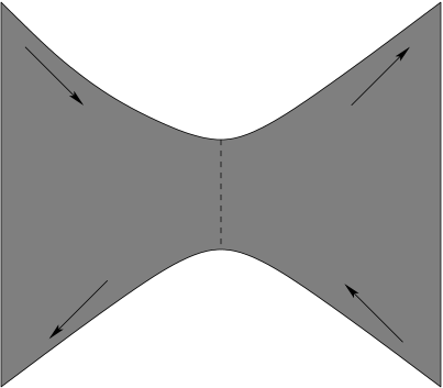
Figure 6: A schematic diagram of the quantum Hall bar system with a “constriction” which promotes quasiparticle tunneling between two points on oppositely directed edges of the system (dashed line). The upper and lower edges are continuous everywhere and therefore have boundary conditions on the field $\phi$ and its spatial derivative $\partial_{x}\phi$ as given above in equns.(25).

Similarly, for the case of $\nu_{2}=0$, the commutation relation for the transmitting edge states vanishes, killing its dynamics: they carry no current, while the reflecting edge states perfectly convey all incoming current into the outgoing arms on the same side of the constriction. Thus, the matching conditions eqs.(22) at the four corners are reduced to

$$\phi^{1,in}(x=-a) = \phi^{l}(y=-a)~{},~{}\phi^{l}(a)=\phi^{2out}(x=-a),$$

$$\phi^{2,in}(x=a) = \phi^{r}(y=a)~{},~{}\phi^{r}(-a)=\phi^{1out}(x=a),$$

$$\partial_{x}\phi^{1,in}(-a) = \partial_{y}\phi^{l}(-a)~{},~{}\partial_{y}\phi^{l}(a)=\partial_{x}\phi^{2out}(-a),$$

$$\partial_{x}\phi^{2,in}(a) = \partial_{y}\phi^{r}(a)~{},~{}\partial_{y}\phi^{r}(-a)=\partial_{x}\phi^{1out}(a).$$ (26)

Again, these identifications of the fields and their spatial derivatives lead to the continuity conditions which underpin the hydrodynamic theory of Wen wen ; kane for the case of the infinite chiral edges (say, left and right) of two distinct Hall bubbles (each with filling factor $\nu_{1}$) separated by vacuum, and again reproduce the familiar Kac-Moody commutation relations everywhere along the edges. This is shown in Fig.(6) below.

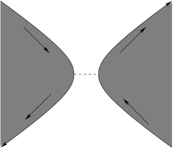
Figure 7: A schematic diagram of a system of two quantum Hall droplets separated by vacuum and with a “constriction” which promotes electron tunneling between two points on adjacent (and oppositely directed) edges of the system (dashed line). The right and left edges are continuous everywhere and therefore have boundary conditions on the field $\phi$ and its spatial derivative $\partial_{x}\phi$ as given above in equns.(26).

We have, in this way, constructed a family of free theories describing ballistic transport through the constriction at intermediate transmission, with those of complete transmission and reflection representing two special cases. This represents an importance advance in generalising the quantum impurity model of refs.kane ; fendley .

III.2.2 Action formulation

In this subsection, we discuss the action (or Lagrangian) formulation of our problem. We will, in this way, demonstrate how the information content of the matching conditions above is already encoded in the action of the system in the forms of terms involving the local fields which are connected to one another by the matching conditions in the Hamiltonian formalism. Thus, we begin by writing down the action for the constriction model

$$S=S_{0}+S_{1}+S_{2}$$ (27)

where the action for the outer incoming and outgoing arms is

$$S_{0} = \int_{0}^{\beta}d\tau\int_{-\infty}^{-a}dx\{{\cal L}_{0}[\phi_{i}^{1,in}]+{\cal L}_{1}[\phi_{i}^{2,out}]\}$$ (28)

$$+\int_{0}^{\beta}d\tau\int_{a}^{\infty}dx\{{\cal L}_{0}[\phi_{i}^{1,out}]+{\cal L}_{1}[\phi_{i}^{2,in}]\}$$

where

$${\cal L}_{0}[\phi^{\alpha}] = \frac{1}{4\pi}\partial_{x}\phi^{\alpha}(i\partial_{\tau}+v\partial_{x})\phi^{\alpha}(x,\tau)~{},$$

$${\cal L}_{1}[\phi^{\alpha}] = \frac{1}{4\pi}\partial_{x}\phi^{\alpha}(-i\partial_{\tau}+v\partial_{x})\phi^{\alpha}(x,\tau)~{},$$ (29)

and we have normalised the entire action with regards to the bulk filling-fraction $\nu_{1}$. Further, the action for the inner edges is

$$S_{1}=\int_{0}^{\beta}\int_{-a}^{a} [ \frac{f}{4\pi}\partial_{x}\phi^{u}(i\partial_{\tau}+v\partial_{x})\phi^{u}(x,\tau)$$ (30)

$$+\frac{f}{4\pi}\partial_{x}\phi^{d}(-i\partial_{\tau}+v\partial_{x})\phi^{d}(x,\tau)$$

$$+\frac{g}{4\pi}\partial_{y}\phi^{l}(i\partial_{\tau}+v\partial_{y})\phi^{l}(y,\tau)$$

$$+\frac{g}{4\pi}\partial_{y}\phi^{r}(-i\partial_{\tau}+v\partial_{y})\phi^{r}(y,\tau)]~{},$$

where, by assuming that the properties of the upper and lower edge transmitted edge states of the constriction are determined by the effective filling-fraction inside the constriction $\nu_{2}$, the quantity $f$ is simply given by $f=\nu_{1}/\nu_{2}$. The quantity $g=\nu_{1}/\nu_{ref}$ (where $\nu_{ref}$ is the effective filling-fraction for the reflected edge states on the left and right) will be determined from the analysis presently. It is worth noting that the same information can be obtained from the Hamiltonians (equns.(18)) and commutation relations (equns.(20))together. Finally, the action for the corner nodes is given by

$$S_{2}=-\int_{0}^{\beta}d\tau\int_{-a}^{a}dx\int_{-a}^{a}dy$$

$$[\delta(x+a)\delta(y+a)\partial_{x}\phi^{1in}\{(v\partial_{x}\phi^{u}+\partial_{y}\phi^{l})+i\partial_{\tau}(\phi^{u}+\phi^{l})\}$$

$$+\delta(x-a)\delta(y+a)\partial_{x}\phi^{1out}\{(v\partial_{x}\phi^{u}+\partial_{y}\phi^{r})+i\partial_{\tau}(\phi^{u}+\phi^{r})\}$$

$$+\delta(x-a)\delta(y-a)\partial_{x}\phi^{2in}\{(v\partial_{x}\phi^{d}+\partial_{y}\phi^{r})-i\partial_{\tau}(\phi^{d}+\phi^{r})\}$$

$$+\delta(x+a)\delta(y-a)\partial_{x}\phi^{2out}\{(v\partial_{x}\phi^{d}+\partial_{y}\phi^{l})-i\partial_{\tau}(\phi^{d}+\phi^{l})\}]~{}.$$ (31)

We can now see the effects of these local terms in the action by computing the equations of motion for the various fields from the action. For the sake of brevity, we carry out this exercise at only the upper-left corner. The results obtained from the other three corners are precisely the same. Thus, we first compute the equation of motion of the “outer” field $\phi_{1in}(x=-a)$ by extremising the action $S$ with regards to $\partial_{x}\phi^{1in}(x=-a)$

$$\frac{\delta S}{\delta(\partial_{x}\phi^{1in}_{-a})} = v(\partial_{x}\phi^{1in}-\partial_{x}\phi^{u}-\partial_{y}\phi^{l})$$ (32)

$$+i\partial_{\tau}(\phi^{1in}-\phi^{u}-\phi^{l})=0$$

where we have suppressed the dependences of the fields on the spatial coordinates for the sake of compactness. From this, we can immediately see the matching conditions on $\phi$ and $\partial_{x}\phi$ at $(x=-a,y=-a)$ given earlier. We now compute the other two equations of motion at the top left corner in the same way. We find, thus,

$$\frac{\delta S}{\delta(\partial_{x}\phi^{u}_{-a})} = v(f\partial_{x}\phi^{u}-\partial_{x}\phi^{1in})$$

$$+i\partial_{\tau}(f\phi^{u}-\phi^{1in})=0$$

$$\frac{\delta S}{\delta(\partial_{y}\phi^{l}_{-a})} = v(g\partial_{y}\phi^{l}-\partial_{x}\phi^{1in})$$ (33)

$$+i\partial_{\tau}(g\phi^{l}-\phi^{1in})=0~{},$$

from which we can see that the currents $j^{u}(x=-a)$ and $j^{l}(y=-a)$ are given by

$$j^{u}(x=-a) = -i\partial_{\tau}(\phi^{u}+\frac{\phi^{1in}}{f})$$

$$= v(\phi^{u}-\frac{\phi^{1in}}{f})\equiv v\rho^{u}(x=-a)$$

$$j^{l}(y=-a) = i\partial_{\tau}(\phi^{l}+\frac{\phi^{1in}}{g})$$ (34)

$$= v(\phi^{l}-\frac{\phi^{1in}}{g})\equiv v\rho^{l}(y=-a)~{}.$$

In the above relations, the currents $(j^{u},j^{l})$ and corresponding densities $(\rho^{u},\rho^{l})$ are those propagated from the incoming arm $1in$ into the u(pper) and l(eft) edge states respectively. Now, by applying Kirchoff’s law for the conservation of current (or, more generally, the equation of continuity) at the upper left corner junction, $j^{1in}(x=-a)=j^{u}(x=-a)+j^{l}(y=-a)$, we obtain

$$\frac{1}{f}+\frac{1}{g}=1~{},$$ (35)

which for $f=\nu_{1}/\nu_{2}$ gives $g=\nu_{1}/(\nu_{1}-\nu_{2})$. This, then, gives us the effective filling-fraction of the reflected edge states as $\nu_{ref}=\nu_{1}-\nu_{2}$. In this way, we can see that the action $S$ contains all the information content given by the Hamiltonians together with the matching conditions.

IV Boundary theory for the constriction system

In this section, we evaluate the role played by local inter-edge quasiparticle tunneling processes deep inside the constriction region in determining the fate of transport through the constriction. In order to do so, we proceed by first integrating out all bosonic degrees of freedom except the few involved in the tunneling processes. In this way, we are left with an effective boundary theory  kane . Given that we have a Gaussian action in terms of the bosonic fields, integrating out various bosonic degrees of freedom can be easily accomplished by performing Gaussian integrations  gogolin ; giamarchi . (another analogous method involves using the solutions to the equations of motion  kane ; lalcontacts ). As this is a very standard procedure, we refer the reader to Refs.(gogolin ; giamarchi ) for details. We pass instead to presenting the various boundary theories obtained in our model, revealing in turn the two interedge quasiparticle tunneling processes which compete in determining the low energy dynamics of the system.

Now, as long as there is no quantum coherence across the constriction region, it is easily seen that the problem of weak, local quasiparticle tunneling between the upper (u) and lower (it d) edges deep inside the constriction region (at, say, $x=0$) is exactly the same as that of local quasiparticle tunneling between the oppositely directed edges of a homogeneous quantum Hall bar with filling fraction $\nu_{2}$  kane . Importantly, the charge and statistics of the quasiparticles undergoing such tunneling processes should be governed by the local filling fraction $\nu_{2}$ alone. Thus, in the action formalism presented earlier, such a quasiparticle tunneling process can be added to the action $S$ by the term $\lambda_{1}\cos(\sqrt{\nu_{1}}(\phi^{u}(0)-\phi^{d}(0)))\equiv\lambda_{1}\cos(\phi^{ud}(0))$, where the tunnel coupling strength is given by $\lambda_{1}$. Integrating out all bosonic degrees of freedom but $\phi^{ud}(x=0)$, we obtain the familiar Kane-Fisher type boundary theory  kane

$$S_{ud}=\sum_{{\bar{\omega}}_{n}}\frac{|{\bar{\omega}}_{n}|}{2\pi\nu_{2}}|\phi^{ud}_{{\bar{\omega}}_{n}}(x=0)|^{2}+\int d\tau\lambda_{1}\cos(\phi^{ud}(x=0,\tau)).$$ (36)

Applying a standard RG procedure, we find the RG equation for $\lambda_{1}$ as

$$\frac{d\lambda_{1}}{dl}=(1-\nu_{2})\lambda_{1}~{}.$$ (37)

As $\nu_{2}<1$, the coupling $\lambda_{1}$ is found to be RG relevant and will grow under the flow to low energies/long lengthscales. Further, this quasiparticle tunneling process will clearly lower the transmission conductance across the constriction $g_{1in,1out}$ (for a source-drain bias as shown in Fig.(2)).

We have, however, at least one other local quasiparticle tunneling process to account for: it is that between the left (l) and right (r) edges of the constriction and is revealed by the generalised quasiparticle-quasihole symmetry of the ground-state in the lowest Landau level (LLL) girvin ; epl . This symmetry dictates that all properties of a quantum Hall system composed of quasiparticles in a partially filled lowest Landau level and with a filling factor $\nu_{qp}$ can be equivalently described by those of a quantum Hall system composed of quasiholes and with a filling factor $\nu_{qh}=1-\nu_{qp}$. This simple relation between $\nu_{qp}$ and $\nu_{qh}$ can be derived easily for the case of the filling factor (and, hence, electronic density) of the quantum Hall system deviating from a filling factor of $\nu_{0}=1/q$ (where $q=2n+1\in{\cal Z}$)  yoshioka . To see this, first note that by increasing the electronic density of the system, we add $q$ quasiparticles for each electron added. Then, for $n_{0}$ being the original electronic density, $n_{e}$ the new increased electronic density and $n_{qp}$ the density of quasiparticles,

$$n_{e}=n_{0}+\frac{n_{qp}}{q}=\frac{\nu_{0}}{2\pi l_{B}^{2}}+\frac{\nu_{0}\nu_{qp}}{2\pi l_{B}^{2}}~{},$$ (38)

where $l_{B}$ is the magnetic length and we have used $n_{0}=\nu_{0}/(2\pi l_{B}^{2})$. This gives us the quasiparticle filling factor $\nu_{qp}$ as

$$\nu_{qp}=\frac{\nu_{e}}{\nu_{0}}~{},$$ (39)

where $\nu_{e}=2\pi l_{B}^{2}n_{e}$ is the electronic filling factor. A similar calculation for the case of an equally lowered value of the electronic density $n_{e}$ can also be carried out. We must now remember that we add $q$ quasiholes to the system for every electron removed. Then, by following the same line of arguments, we get the quasihole filling factor $\nu_{qh}$ as

$$\nu_{qh}=1-\frac{\nu_{e}}{\nu_{0}}=1-\nu_{qp}~{}.$$ (40)

Thus, we can see that $\nu_{qp}$ and $\nu_{qh}$ are related by a quasiparticle-quasihole conjugation transformation. Further, for the case of $\nu_{0}=1$, $\nu_{qp}=\nu_{e}$ and $\nu_{qh}=\nu_{h}=1-\nu_{e}$ are the well-known electron and hole conjugation symmetric filling factors with respect to the completely filled lowest electronic Landau level  girvin .

The application of this symmetry to the constriction model with a spatially dependent filling fraction relies on (a) the fact that the fractional (integer) quantum Hall ground state in the bulk of the system can be thought of as the completely filled effective lowest Landau level of quasiparticles (electrons), (b) that this state is protected by an energy gap which is larger than all other energy scales in the problem and (c) there is no Landau level mixing. While the argument for a constriction circuit with the bulk being in the integer quantum Hall state of $\nu_{1}=1$ has been given in Ref.(roddaro1 ), a generalisation for any constriction circuit with a general bulk filling factor $\nu_{1}<1$ was presented in Ref.(epl ). The argument is recounted below and encapsulated in Fig.(8).

\psfrag{1}[bl][bl][5][0]{$\frac{\nu_{2}}{\nu_{1}}$}\psfrag{2}[bl][bl][4][0]{$0$}\psfrag{3}[bl][bl][4][0]{$0$}\psfrag{4}[bl][bl][4][0]{$1$}\psfrag{5}[bl][bl][4][0]{$1$}\psfrag{6}[bl][bl][4][0]{(a)}\psfrag{7}[bl][bl][4.9][0]{$1-\frac{\nu_{2}}{\nu_{1}}$}\psfrag{8}[bl][bl][4][0]{$1$}\psfrag{9}[bl][bl][4][0]{$1$}\psfrag{10}[bl][bl][4][0]{$0$}\psfrag{11}[bl][bl][4][0]{$0$}\psfrag{12}[c][c][4][0]{(b)}\psfrag{13}[c][c][4][0]{(c)}\psfrag{14}[c][c][4][0]{(d)}\includegraphics{fig8.eps}

Figure 8: The quasiparticle-quasihole (qp-qh) symmetry of the $(\nu_{1},\nu_{2})$ constriction geometry in terms of the relative filling factor. The source-drain bias $2V_{in}$ is applied to the two incoming arms while $\pm V_{out}$ are the equilibration potentials of the two outgoing arms. See text for a detailed description of the transformations linking (a) to (d).

By scaling the filling factors of all regions by $\nu_{1}$, we now have the effective filling factor of the bulk as $1$ and that of the quantum Hall ground state inside the constriction region as the relative filling fraction $f^{-1}=\nu_{2}/\nu_{1}$. Carrying out the qparticle-qhole conjugation transformation, we go to a system of holes (with the direction of the external magnetic field unaffected) but with the relative filling fraction of the constriction now given by $g^{-1}=1-f^{-1}$. We can then map this system of qholes onto that of time-reversed qparticles (i.e., qparticles in an oppositely directed external magnetic field). Finally, by rotating the system by $180^{o}$ around the axis of the two outgoing current directions, we are left with a system of electrons with the external magnetic field pointing in the original direction. This final system is, however, crucially different in two ways from the original one. First, the filling factor of the fractional quantum Hall ground state inside the constriction region has, as noted earlier, changed from $f^{-1}$ to $g^{-1}=1-f^{-1}$. Second, the directions transmitted and reflected currents has been interchanged in going from the original system to the final one. It is easy to show that current conservation dictates that roddaro1

$$I_{f^{-1}}+I_{g^{-1}}=2\nu_{1}\frac{e^{2}}{h}V_{in}~{},$$ (41)

where $I_{f^{-1}}$ and $I_{g^{-1}}$ are the transmitted currents in the original system and the final system after the mappings (i.e., the reflected current in the original system). Relations can also be written down in terms of differential transmission $t=dI/dV$ and reflection $r$ (in units of $\nu_{1}e^{2}/h$)

$$t_{f^{-1}} = 1-t_{g^{-1}}=r_{g^{-1}}$$

$$t_{g^{-1}} = 1-t_{f^{-1}}=r_{f^{-1}}~{}.$$ (42)

This argument also clearly demonstrates that the local tunneling process that transports these qholes between the left (l) and right (r) edges of the constriction system is governed by the effective filling-fraction of $g^{-1}=1-\nu_{2}/\nu_{1}$. Thus, we denote such a local tunneling process (again, chosen at $y=0$) on the l and r edges by a weak tunnel coupling $\lambda_{2}$ and a term in the action $S$, $\lambda_{2}\cos(\phi^{l}(0)-\phi^{r}(0))\equiv\lambda_{2}\cos(\phi^{lr}(0))$. Integrating out all bosonic degrees of freedom but $\phi^{lr}(y=0)$, we obtain the another Kane-Fisher type boundary theory  kane

$$S_{lr}=\sum_{{\bar{\omega}}_{n}}\frac{|{\bar{\omega}}_{n}|}{2\pi g}|\phi^{lr}_{{\bar{\omega}}_{n}}(y=0)|^{2}+\int d\tau\lambda_{2}\cos(\phi^{lr}(y=0,\tau))~{}.$$ (43)

Thus, we can see that the RG equation for the coupling $\lambda_{2}$ is given by

$$\frac{d\lambda_{2}}{dl} = (1-\frac{1}{g})\lambda_{2}$$ (44)

$$= (1-(1-\frac{\nu_{2}}{\nu_{1}}))\lambda_{2}=\frac{\nu_{2}}{\nu_{1}}\lambda_{2}~{}.$$

As both $(\nu_{1},\nu_{2})>1$ and $\nu_{2}<\nu_{1}$, we can see that the coupling $\lambda_{2}$ is also RG relevant and will grow under the flow to low energies/long lengthscales. Further, this tunneling process will increase the transmission conductance $g_{1in,1out}$.

Since we have two RG relevant boundary operator couplings which affect the transmission conductance across the constriction in opposite ways, we need to determine the conditions under which one wins over the other. From the scaling dimensions of the two operators (as employed in their respective RG equations), we can see that the two couplings grow equally fast for a critical $\nu^{*}_{2}$

$$\nu^{*}_{2}=\frac{\nu_{1}}{1+\nu_{1}}~{}.$$ (45)

For this critical $\nu^{*}_{2}$, then, the transmission and reflection conductances will be held fixed by the generalised qparticle-qhole symmetry all along the RG flow from weak to strong coupling! For $\nu_{2}<\nu^{*}_{2}$, $\lambda_{1}$ dominates over $\lambda_{2}$, which will lead to a minimum of the transmission conductance (i.e., a maximum in the reflection conductance) at low energies (bias/temperature) given by the bulk conductance $\nu_{1}$. The quantum Hall constriction system will then resemble that of two quantum Hall droplets separated by vacuum, shown in Fig.(7) above. Similarly, for $\nu_{2}>\nu^{*}_{2}$, $\lambda_{2}$ dominates over $\lambda_{1}$ and will lead to the opposite case of a maximum in the transmission conductance (i.e., a minimum in the reflection conductance) at low energies (bias/temperature) given by the bulk conductance $\nu_{1}$. The quantum Hall constriction system will then resemble that of a single quantum Hall bar, shown in Fig.(6) above. As was discussed in detail in an earlier section, these were indeed many of the puzzling experimental findings of Refs. roddaro1 ; roddaro2 ; chung .

We can see that, for the critical value of $\nu^{*}_{2}$ predicted by our theory, the symmetry-determined (i.e., energy scale independent) constriction transmission conductance is given by

$$t(\nu^{*}_{2}) = \frac{g_{1in,1out}(\nu^{*}_{2})}{G_{b}}=\frac{\nu^{*}_{2}}{\nu_{1}}=\frac{1}{1+\nu_{1}}$$ (46)

$$= 1-\nu_{2}^{*}~{}.$$

We now present the above results for the first three generations of the heirarchical sequence of quantum Hall states.
(i) For the bulk filling-factor belonging to the primary sequence $\nu_{1}=1/(2p-1)$, we obtain

$$\nu^{*}_{2}=\frac{1}{2p}~{}~{},~{}~{}t(\nu^{*}_{2})=\frac{2p-1}{2p}~{}.$$ (47)

Specifically, for $\nu_{1}=1$, we get $\nu^{*}_{2}=1/2=t(\nu^{*}_{2})$ and for $\nu_{1}=1/3$, we get $\nu^{*}_{2}=1/4$, $t(\nu^{*}_{2})=3/4$. Both these sets of results match the experimental findings of Refs. roddaro1 ; roddaro2 ; chung .
(ii)Further, we find that for the case of the second generation of the heirarchical states, $\nu_{1}=2p/(2pq\pm 1)$ (where $p=1$,$q=3,5,\ldots$), we find

$$\nu_{2}^{*}=\frac{2p}{2p(1+q)\pm 1}~{}~{},~{}~{}t(\nu_{2}^{*})=\frac{2pq\pm 1}{2p(1+q)\pm 1}~{}.$$ (48)

Specifically, for the case of $\nu_{1}=2/5$, $\nu_{2}^{*}=2/7$ and $t(\nu_{2}^{*})=5/7$.
(iii) Extending these results to the third generation of the heirarchical states, $\nu_{1}=4p_{1}p_{2}/(q(4p_{1}p_{2}\pm 1)\pm 2p_{2})$ (where $p_{1}=1=p_{2}$,$q=3,5,\ldots$), we obtain

$$\nu_{2}^{*} = \frac{4p_{1}p_{2}\pm 1}{((1+q)(4p_{1}p_{2}\pm 1)\pm 2p_{2})}~{},$$

$$t(\nu_{2}^{*}) = \frac{q(4p_{1}p_{2}\pm 1)\pm 2p_{2}}{(1+q)(4p_{1}p_{2}\pm 1)\pm 2p_{2}}~{}.$$ (49)

Specifically, for the case of $\nu_{1}=3/7$, $\nu_{2}^{*}=3/10$ and $t(\nu_{2}^{*})=7/10$. The results presented for the cases of $\nu_{1}=2/5,3/7$ can be tested experimentally, and we will comment on this in a later section.

\psfrag{1}[bl][bl][4][0]{$\ln\lambda_{1}$}\psfrag{2}[bl][bl][4][0]{$\ln\lambda_{2}$}\psfrag{3}[bl][bl][4][0]{$\nu_{2}<\nu_{2}^{*}$}\psfrag{4}[bl][bl][4][0]{$\nu_{2}>\nu_{2}^{*}$}\psfrag{5}[bl][bl][4][0]{$\nu_{2}=\nu_{2}^{*}$}\includegraphics{fig9.eps}

Figure 9: The RG phase diagram for the model as a plot of the function $\ln\lambda_{1}/\ln\lambda_{2}=\nu_{1}(1/\nu_{2}-1)$. All RG flows lead away from the weak-coupling unstable fixed point at the origin. Properties of the dashed critical line and regions above $(\nu_{2}<\nu_{2}*)$ and below $(\nu_{2}>\nu_{2}^{*})$ are explained in the text.

Finally, we present the RG phase diagram of the model in Fig.(9) given above. The origin represents the family of weak-coupling fixed point theories at partial transmission described earlier, while the RG flows are to the familiar fixed point theories kane ; fendley of complete reflection ($\nu_{2}<\nu_{2}^{*}$, see Fig.(7) given above), complete transmission ($\nu_{2}>\nu_{2}^{*}$, see Fig.(6) given above) and to a new symmetry dictated fixed point theory on the diagonal ($\nu_{2}=\nu_{2}^{*}$). The diagonal is, in fact, a separatrix – a line of gapless critical theories all possessing the quasiparticle-quasihole symmetry described above – dividing RG flows to a metallic phase (as evidenced by the perfect transmission through the constriction) and an insulating phase (as seen by the perfect reflection at the constriction) at strong coupling. The qparticle-qhole symmetry of the constriction system can also be seen in the reflection symmetry of the RG flows in the two segments on either side of the separatrix: in physical terms, this means that while the upper (lower) segment represent RG flows towards a qparticle insulator (metal), the picture is exactly reversed for a description in terms of qholes. This is also amply clear in terms the comparison of the two scaling dimensions: this analysis answers the question as to which of the qparticle and qhole boundary degrees of freedom (given above in the two boundary theories for qparticle and qhole tunneling respectively) becomes massive first, thereby allowing the remaining gapless boundary degrees of freedom to determine the low energy, long wavelength dynamics of the quantum Hall constriction system at strong coupling. Finally, this symmetry of the RG phase diagram is reminiscent of the edge-state transmission duality shimshoni ; xiong that is known to exist in the Chalker-Coddington model chalcodd as applied to the study of the quantum Hall transitions.

The novel structure of the RG phase diagram, thus, reflects on the fact that the experimentally observed gate-voltage tuned metal-insulator transition (at vanishing edge bias) is in fact shaped not only by boundary critical phenomena (i.e., local interedge quasiparticle tunneling processes, relying on an interplay of the physics of impurity scattering and electron electron interactions  kane ), but also by the presence of a global symmetry (i.e., the quasiparticle-quasihole conjugation symmetry) and the requirement of overall current conservation in the system. These findings highlight the novel generalisation of the quantum impurity problem of refs.kane ; fendley that has been accomplished here. We can now proceed to a study of the correlators and conductances of the system in the next section, with an effort towards reinforcing the physical picture presented by these RG flows.

V Correlators and conductances of the constriction model

In this section, we present computations of various density-density correlators of the fields in the constriction model for the three cases of weak coupling ballistic transport (i.e., no interedge tunneling), strong coupling with interedge tunneling for $\nu_{2}<\nu_{2}^{*}$ and strong coupling with interedge tunneling for $\nu_{2}>\nu_{2}^{*}$. We then employ these correlators in a Kubo formulation to compute the chiral linear dc conductances of the system. In this way, we will confirm the physical picture of the dip-to-peak evolution developed in the last section. We will, in this way, also be able to see the consequence of the qparticle-qhole symmetry on measurable quantities like conductances, confirming the physical picture of transport through the constriction system presented earlier.

In all that follows, we switch from the Euclidean time $\tau$ to Matsubara frequencies ${\bar{\omega}}_{n}$. This will also be seen to facilitate the computation of the the linear dc conductances. Thus, we begin by computing certain density-density correlators, e.g., $\langle[\partial_{x}\phi^{1in}_{{\bar{\omega}}_{n}}(x),\partial_{x}\phi^{1out}_{-{\bar{\omega}}_{n}}(x^{\prime})]\rangle$, for the free theory $S$ given earlier (i.e., $S$ in the absence of all interedge tunneling processes)

$$\langle[\partial_{x}\phi^{1in}_{{\bar{\omega}}_{n}}(x),\partial_{x}\phi^{1out}_{-{\bar{\omega}}_{n}}(x^{\prime})]\rangle=$$

$$\langle[(\partial_{x}\phi^{u}_{-a}+\partial_{y}\phi^{l}_{-a})(\partial_{x}\phi^{u}_{a}+\partial_{y}\phi^{r}_{-a})]\rangle e^{-|{\bar{\omega}}_{n}(x^{\prime}-x-2a)/v|}$$

$$=\langle[\partial_{x}\phi^{u}_{-a},\partial_{x}\phi^{u}_{-a}]\rangle e^{-|{\bar{\omega}}_{n}(x^{\prime}-x)/v|}$$

$$=\frac{2\pi\nu_{2}}{v^{2}}|{\bar{\omega}}_{n}|e^{-|{\bar{\omega}}_{n}(x^{\prime}-x)/v|}~{},$$ (50)

where we have used the commutation relations for the various fields and the fact that all transport on the various edges is ballistic and described by the solutions to the chiral equations of motion for the edge density waves given earlier. Further, for the sake of notational brevity, we suppressed the ${\bar{\omega}}_{n}$ frequencies in all subscripts on the right hand side, keeping only the spatial dependence in the subscripts in the correlator expressions. The $e^{-|{\bar{\omega}}_{n}(x^{\prime}-x)/v|}$ factor is the expected phase (easily seen upon performing an analytic continuation to real frequencies $\omega$) associated with the ballistic transport between the points $x$ and $x^{\prime}$. As we will soon see when deriving the expressions for the linear dc conductances, this phase factor vanishes upon taking the limit of vanishing frequencies, while the filling factor dependence is crucial.

In the same way, we find the other density-density correlators between the fields outside the constriction as

$$\langle[\partial_{x}\phi^{1in}_{{\bar{\omega}}_{n}}(x),\partial_{x}\phi^{2out}_{-{\bar{\omega}}_{n}}(x^{\prime})]\rangle=-\frac{2\pi(\nu_{1}-\nu_{2})}{v^{2}}|{\bar{\omega}}_{n}|e^{-|{\bar{\omega}}_{n}(x^{\prime}-x)/v|},$$

$$\langle[\partial_{x}\phi^{2in}_{{\bar{\omega}}_{n}}(x),\partial_{x}\phi^{2out}_{-{\bar{\omega}}_{n}}(x^{\prime})]\rangle=-\frac{2\pi\nu_{2}}{v^{2}}|{\bar{\omega}}_{n}|e^{-|{\bar{\omega}}_{n}(x^{\prime}-x)/v|}~{},$$

$$\langle[\partial_{x}\phi^{2in}_{{\bar{\omega}}_{n}}(x),\partial_{x}\phi^{1out}_{-{\bar{\omega}}_{n}}(x^{\prime})]\rangle=\frac{2\pi(\nu_{1}-\nu_{2})}{v^{2}}|{\bar{\omega}}_{n}|e^{-|{\bar{\omega}}_{n}(x^{\prime}-x)/v|}.$$ (51)

We now turn to the case of strong coupling interedge tunneling within the constriction. Here, three scenarios can be realised, and we study each of them in turn. First, for the case of $\nu_{2}<\nu_{2}^{*}$, we have already seen that quasiparticle tunneling between the upper and lower edges of the constriction region dominates at strong coupling. Then, from the boundary theory given earlier, it is clear that this strong coupling scenario possesses another boundary condition (dynamically generated due to the RG flow): $\phi^{u}(x=0)=\phi^{d}(x=0)$. Using this boundary condition while computing the four density-density correlators given above, we find

$$\langle[\partial_{x}\phi^{1in}_{{\bar{\omega}}_{n}}(x),\partial_{x}\phi^{1out}_{-{\bar{\omega}}_{n}}(x^{\prime})]\rangle=0~{},$$

$$\langle[\partial_{x}\phi^{1in}_{{\bar{\omega}}_{n}}(x),\partial_{x}\phi^{2out}_{-{\bar{\omega}}_{n}}(x^{\prime})]\rangle=-\frac{2\pi\nu_{1}}{v^{2}}|{\bar{\omega}}_{n}|e^{-|{\bar{\omega}}_{n}(x^{\prime}-x)/v|}~{},$$

$$\langle[\partial_{x}\phi^{2in}_{{\bar{\omega}}_{n}}(x),\partial_{x}\phi^{2out}_{-{\bar{\omega}}_{n}}(x^{\prime})]\rangle=0~{},$$

$$\langle[\partial_{x}\phi^{2in}_{{\bar{\omega}}_{n}}(x),\partial_{x}\phi^{1out}_{-{\bar{\omega}}_{n}}(x^{\prime})]\rangle=\frac{2\pi\nu_{1}}{v^{2}}|{\bar{\omega}}_{n}|e^{-|{\bar{\omega}}_{n}(x^{\prime}-x)/v|}~{}.$$ (52)

It is easy to see from these correlators that the physical system here is that visualised in Fig.(7).

Next, for the case of $\nu_{2}>\nu_{2}^{*}$, we have already determined that quasiparticle tunneling between the left and right edges of the constriction region dominates at strong coupling. Then, from the boundary theory given earlier, it is clear that this strong coupling scenario possesses another boundary condition (again, dynamically generated due to the RG flow): $\phi^{l}(y=0)=\phi^{r}(y=0)$. Using this boundary condition while computing the four density-density correlators given above, we find

$$\langle[\partial_{x}\phi^{1in}_{{\bar{\omega}}_{n}}(x),\partial_{x}\phi^{1out}_{-{\bar{\omega}}_{n}}(x^{\prime})]\rangle=\frac{2\pi\nu_{1}}{v^{2}}|{\bar{\omega}}_{n}|e^{-|{\bar{\omega}}_{n}(x^{\prime}-x)/v|},$$

$$\langle[\partial_{x}\phi^{1in}_{{\bar{\omega}}_{n}}(x),\partial_{x}\phi^{2out}_{-{\bar{\omega}}_{n}}(x^{\prime})]\rangle=0~{},$$

$$\langle[\partial_{x}\phi^{2in}_{{\bar{\omega}}_{n}}(x),\partial_{x}\phi^{2out}_{-{\bar{\omega}}_{n}}(x^{\prime})]\rangle=-\frac{2\pi\nu_{1}}{v^{2}}|{\bar{\omega}}_{n}|e^{-|{\bar{\omega}}_{n}(x^{\prime}-x)/v|}~{},$$

$$\langle[\partial_{x}\phi^{2in}_{{\bar{\omega}}_{n}}(x),\partial_{x}\phi^{1out}_{-{\bar{\omega}}_{n}}(x^{\prime})]\rangle=0~{}.$$ (53)

It is again easy to see from these correlators that the physical system here is that visualised in Fig.(6).

Finally, we turn to considering the qparticle-qhole symmetric case of $\nu_{2}=\nu_{2}^{*}$. It is clear that since the two RG flows to strong coupling indicate opposing tendencies on the system, i.e., very different physical configurations for the system (Figs.(6) and (7) respectively), the equally fast growth of both couplings still cannot lead to the generation of any new boundary conditions in this case. It is then easily concluded that all the density-density correlators studied above must appear to be exactly the same at strong coupling as found to be at weak coupling (and, indeed, all along the RG flow). Thus, the consequence of the global symmetry of qparticle-qhole conjugation is to keep the various transmission and reflection edge fields at the constriction from becoming massive locally. This confirms the existence of a line of critical (gapless) theories, all possessing the symmetry mentioned above and unstable to relevant RG perturbations upon changing the parameter $\nu_{2}$ from its critical value; the correlators confirm that the RG flow is towards strong coupling theories where either the transmitting or the reflecting edges become massive locally, suppressing some of the correlators while giving the other correlators the values they would have in the two scenarios in Figs.(6) and (7).

As we will now see, by using the fact that the charge and current densities for a chiral edge bosonic field $\phi$ are simply related to another another, these density-density correlators can be employed in computing several 2-terminal chiral linear (dc) conductances. These conductances can be derived from a linear response type Kubo formulation  kane ; moon ; kanefishreview , yielding relations linking them to the correlators computed above in the form of retarded response functions (obtained upon performing an analytic continuation from Matsubara frequencies ${\bar{\omega}}_{n}$ to real frequencies $\omega$)

$$g_{\alpha\beta}(x,x^{\prime}) = \lim_{\omega\rightarrow 0}(-1)^{[\tilde{\alpha}+\tilde{\beta}]}\frac{e^{2}v^{2}}{2\pi h\omega}\times$$ (54)

$$\hskip 5.69046pt\times\langle[\partial_{x}\phi^{\alpha}_{\omega}(x),\partial_{x}\phi^{\beta}_{-\omega}(x^{\prime})]\rangle~{},$$

where $(\alpha,\beta)=(1in,\ldots,2out)$ are the terminal indices, $(\tilde{\alpha},\tilde{\beta})$ are the terminal numbers (i.e., $1$ and $2$) associated with these terminal indices and $[\tilde{\alpha}+\tilde{\beta}]$ is a number modulo $2$ such that the factor $(-1)^{[\tilde{\alpha}+\tilde{\beta}]}$ restores the direction of net current flow from source to drain as positive. From the expressions for the correlators given earlier, it is clear that in the dc limit $\omega\rightarrow 0$ , the linear conductances no longer depend on the spatial coordinates of $x$ and $x^{\prime}$; this is a consequence of the fact that transport along the edges is ballistic and equilibriation takes place only in the reservoirs  kanefishreview . We can now simply use the various correlators computed above in calculating the various 2-terminal chiral linear conductances of the system. For the sake of brevity, we summarise in table (1) presented below, our calculations of the chiral linear conductances $g_{1in,1out}$ and $g_{1in,2out}$, representing the transmission and reflection through the constriction, at weak coupling (ballistic transport only) and the three strong coupling scenarios of $\nu_{2}<\nu_{2}^{*}$, $\nu_{2}>\nu_{2}^{*}$ and $\nu_{2}=\nu_{2}^{*}$.

Constriction filling          $\nu_{2}$	$g_{1in,1out}(e^{2}/h)$	$g_{1in,2out}(e^{2}/h)$
Weak coupling	$\nu_{2}$	$\nu_{1}-\nu_{2}$
Strong coupling
$(\nu_{2}<\nu_{2}^{*})$	0	$\nu_{1}$
Strong coupling
$(\nu_{2}>\nu_{2}^{*})$	$\nu_{1}$	0
Strong coupling
$(\nu_{2}=\nu_{2}^{*})$	$\nu_{2}$	$\nu_{1}-\nu_{2}$

Table 1: Values of two chiral linear conductances, $g_{1in,1out}$ and $g_{1in,2out}$, representing the transmission and reflection through the constriction at weak coupling (ballistic transport only) and the three strong coupling scenarios of $\nu_{2}<\nu_{2}^{*}$, $\nu_{2}>\nu_{2}^{*}$ and $\nu_{2}=\nu_{2}^{*}$.

The other two conductances $g_{2in,1out}$ and $g_{2in,2out}$ can be computed in precisely the same manner. The physical picture of weak coupling ballistic transport and the three strong coupling scenarios presented earlier is immediately confirmed from the expressions given in table (1). The finite temperature $T$ (or voltage $V$) expressions for the perturbative corrections to the weak coupling ballistic chiral conductances due to the qparticle and qhole interedge tunneling processes revealed earlier can also be computed from the boundary theories presented earlier  kane . Thus, we find that

$$\delta g_{1in,1out}^{WC} = g_{1in,1out}-\nu_{2}\frac{e^{2}}{h}$$

$$= -c_{1}\frac{e^{2}}{h}\lambda_{1}^{2}T^{2\nu_{2}-2}+c_{2}\frac{e^{2}}{h}\lambda_{2}^{2}T^{-2\nu_{2}/\nu_{1}}$$

$$\delta g_{1in,2out}^{WC} = g_{1in,2out}-(\nu_{1}-\nu_{2})\frac{e^{2}}{h}$$ (55)

$$= +c_{3}\frac{e^{2}}{h}\lambda_{1}^{2}T^{2\nu_{2}-2}-c_{4}\frac{e^{2}}{h}\lambda_{2}^{2}T^{-2\nu_{2}/\nu_{1}}~{},$$

where $(c_{1},\ldots,c_{4})$ are non-universal constants. We conclude by noting that, for the qparticle-qhole symmetric critical constriction filling factor of $\nu_{2}^{*}$, the tunneling strengths $\lambda_{1}\equiv\lambda_{2}$ while the constants are related as $c_{1}=c_{2}~{},~{}c_{3}=c_{4}$, such that the corrections to the chiral linear conductances given above vanish, $\delta g_{1in,1out}^{WC,\nu_{2}^{*}}=0=\delta g_{1in,2out}^{WC,\nu_{2}^{*}}$ . This provides a more quantitative explanation of the edge-bias independent constriction transmission observed experimentally  roddaro1 .

VI Comparison with the experiments

In this section, we bring together all our results in order to compare them with the findings of the experiments  roddaro1 ; roddaro2 ; chung ; roddaro3 . In our phenomenological model for edge state transport in the presence of a gate-voltage controlled constriction, we have chosen to model the constriction by a mesoscopic region of lowered electronic density (and hence, filling fraction $\nu_{2}$) in comparison to that in the bulk (of filling fraction $\nu_{1}$). The reduced transmission through the constriction at high edge-bias (i.e., partial transmission ballistic transport) is explained in terms of the transmitting edge states of the constriction, whose properties are governed solely by the constriction quantum Hall fluid. Further, the experimentally observed current backscattered from the constriction (and received in a terminal on the opposite side of the Hall bar) is explained in terms of the existence of a gapless edge state lying in between the bulk and constriction quantum Hall fluids (and whose properties are governed by both the bulk as well as the constriction fluids).

Next, the startling dip-to-peak evolution of the vanishing bias constriction transmission with decreasing strength of the gate-voltage is understood as the result of a competition between local interedge quasiparticle (quasihole) tunneling events among the transmitting (reflecting) edges of the constriction region. The edge-bias independent constriction transmission is seen to arise from the qparticle-qhole symmetric critical theories that lie on the separatrix of the RG phase diagram; the equal and opposite growth of the two interedge tunneling processes leads to an exact cancellation of any gap generating processes. These critical theories are characterised by a critical value of $\nu_{2}=\nu_{2}^{*}$ and separate relevant RG flows to either of the cases of perfect and zero transmission through the constriction. The values of the critical $\nu_{2}^{*}$ and the constriction transmission at this value, $t(\nu_{2}^{*})$, are seen to match exactly those obtained experimentally for the cases of the bulk $\nu_{1}=1,1/3$   roddaro1 ; roddaro2 . Further, the experimental finding of $t(\nu_{2}^{*})$ lying between $0.7$ and $0.8$ for both the cases of $\nu_{1}=2/5$ and $\nu_{1}=3/7$  chung appear to be consistent with those obtained from the results obtained from our model. More rigorous experimental investigations of the $\nu_{1}=2/5,3/7$ systems may, however, be necessary to make a firmer statement. Further, the two dip-to-peak evolutions observed for the case of $\nu_{1}=2$  roddaro1 , is easily understood from our model as long as we assume zero inter-Landau level mixing. Finally, the phenomenological assumptions of (i) a constriction region characterised simply by one parameter, $\nu_{2}$, and (ii) only local interedge tunneling events inside the constriction appear to be robust against changes in the size and shape of the constriction (i.e., the size and shape of the gate-voltage plates which create the constriction through electrostatic means); this is consistent with the experimental results of Ref.(roddaro3 ).

We now evaluate the relevance of our model in understanding the findings of a recent work on a constriction circuit with the bulk at $\nu_{1}=3$  miller . In this work, the authors appear to find evidence for a zero-bias resistance peak for the case of the constriction at $\nu_{2}=5/2$. Levin etal., in a very recent work  levin , attribute this to the possibility of a Pfaffian (Pf) $5/2$ state existing in the constriction quantum Hall fluid, rather than its particle-hole conjugate anti-Pfaffian (Apf) state. For this, they appear to use the simple model for the constriction first revealed in Ref.(epl ) (and further elaborated upon here), together with the fact that they find the interedge tunnel coupling between the transmitting edges ($\lambda_{1}$ in our work) to be more RG relevant than the interedge tunnel coupling between the reflecting edges ($\lambda_{2}$ in our work). Thus, this experimental observation  miller appears, at first sight, to be inconsistent with our results for the case of $\nu_{1}=3$: specifically, our analysis predicts that the constriction filling fraction of $\nu_{2}=5/2$ is critical, and the constriction transmission should therefore be edge-bias independent (as observed in the experiments for the cases of $\nu_{2}=1/2,\nu_{1}=1$ and $\nu_{2}=3/2,\nu_{1}=2$  roddaro1 ). While Miller etal.  miller find a zero-bias resistance peak at $\nu_{2}=7/3$ in consistency with the predictions from our analysis, experimental results at $\nu_{2}=8/3$ (where our analysis predicts the existence of a zero-bias resistance minimum) are as yet forthcoming.

A closer look, however, reveals that the inconsistency for the case of $\nu_{2}=5/2$ arises from the following fact. The analysis of the quantum Hall constriction system carried out in the present work relies on the assumption that the quantum Hall ground states in the bulk as well as constriction regions are completely spin polarised, have only two-body interactions, exactly $1/2$-electron per magnetic flux and no inter-Landau level mixing. The Pf state, on the other hand, is the exact ground state of a three-body interaction which explicitly breaks particle-hole symmetry  greiter . It is, therefore, not surprising that the predictions of edge state theories based on these two bulk quantum Hall states should be quite different. A more systematic experimental study of the $\nu_{1}=3$ constriction system along the lines of that conducted by Roddaro etal. for the $\nu_{1}=1$ system  roddaro1 could, therefore, improve considerably our understanding of the nature of the $\nu=5/2$ quantum Hall ground state.

VII Summary and Outlook

In this work, we have introduced a model which describes intermediate conductance scenarios in the problem of tunneling in 1D chiral systems by constructing a model for a constricted region (i.e., with a lower filling fraction, $\nu_{2}$, than that of the Hall fluid in the bulk, $\nu_{1}$). A Landauer-Buttiker analysis of ballistic transport reveals that the constriction acts as a junction for the chiral density waves incident on it by splitting them into currents on the transmitting and reflecting arms of the constriction region. An edge state model is then formulated in terms of a hydrodynamic theory of long-wavelength, low-energy chiral density-wave excitations. Specifically, we are able to describe the dynamics of the constriction junction in terms of two pairs of edge fields, $(\phi^{u},\phi^{d})$ and $(\phi^{l},\phi^{r})$, whose properties are governed by the effective filling fractions $\nu_{2}$ and $\nu_{1}-\nu_{2}$ respectively. The constriction is connected to two incoming- and two outgoing-chiral modes. Introducing local quasiparticle tunneling across various arm pairs of the constriction, we derive the perturbative RG equations for the various tunnel couplings and find that the RG flow is towards strong-coupling for both the tunnel couplings considered. A competition between the two couplings to reach the strong-coupling regime determines the low-energy configuration of the system. A quasiparticle-quasihole symmetry of the system is found to determine the existence of a line of critical (gapless) theories at a critical filling fraction of the constriction region ($\nu_{2}^{*}$) which separates the relevant RG flows towards the perfect transmission and reflection strong coupling fixed point theories. The conductances $g_{1in,1out}$ and $g_{1in,2out}$ are computed in the weak and strong quasiparticle tunneling coupling limits and are also found to match qualitatively the experimental findings of Refs.roddaro1 ; roddaro2 . We are also able to recover the familiar results for $\nu_{2}=\nu_{1}$ kane ; moon . In this way, we have achieved a non-trivial generalisation of the generic phenomenological model of tunneling in FQHE systems formulated by Kane and Fisher kane ; moon .

Given the success the phenomenological edge model proposed in this work meets in providing explanations for the various puzzling experimental observations, we now turn to a discussion of certain aspects of the model. First, the model relies essentially on treating the filling fractions of the quantum Hall ground state in the bulk ($\nu_{1}$) and constriction($\nu_{2}$) regions as the two parameters of the model. While such a model is sensible for the case of when both $(\nu_{1},\nu_{2})$ take values from among the special fractions representing incompressible quantum Hall ground states, how far can we trust it for the case of when the quantum Hall ground states in the bulk and constriction regions are compressible? The answer could lie in a work by Levitov, Shytov and Halperin  levitov provides a generalisation of the chiral TLL edge state to the case of a compressible quantum Hall state in the bulk via a composite-fermion Chern-Simons formulation. Thus, it should be possible to derive the edge model for the constriction system proposed here for a general quantum Hall ground state by proceeding along similar lines.

Further, the multimode nature of the edge state of several members of the incompressible Jain heirarchy of quantum Hall states, involving one charged edge mode and several charge neutral modes, is a well established fact theoretically. Thus, it is worth understanding how the present model (with its assumption of a single edge mode everywhere in the circuit) fares so well in its comparison with the experiments even in describing such quantum Hall states. A possible microscopic explanation can be found by assuming that the velocity of the charge mode is much greater than those of the various neutral modes of a multimode edge state  leewen . Under such circumstances, the dynamics of only the charge edge mode becomes important in an intermediate energy regime, while the responses arising from the various neutral modes can be ignored. Further, the composite fermion field theoretic formulation by Lopez and Fradkin departs from the multimode picture of the QH edge for the incompressible Jain fractions  lopezfradkin ; this construction involves only one charge mode (and two auxiliary Klein factors which do not have any additional propagating degrees of freedom). In this sense, this formulation can be likened to the other multimode edge theories with vanishing neutral mode velocities. Finally, for the case of integer quantum Hall systems, it is worth noting that recent numerical works by Siddiki and co-workers  siddiki suggest that quantum Hall systems at higher (integer) $\nu$ filling fractions generically involve only one edge mode in charge transport.

The present work can clearly be generalised to the case of more than 4 chiral wires meeting at a junction. This is important in modeling the transport across various kinds of junctions of several non-chiral Tomonaga-Luttinger liquid wires, where the RG phase diagram is known to contain several non-trivial fixed points nayak ; lal ; chen ; chamon ; das ; sumadip . Studies of resonant-tunneling junctions (i.e., junctions which possess a resonant two-level system or spin-1/2 degree of freedom in addition to allowing quasiparticle tunneling) kane ; nayak ; chamon ; sumadip reveal interesting transport phenomena (including variations of the Kondo- and Coulomb-blockade effects); a resonant-tunneling constriction junction is likely to possess novel variations of the phenomena found in these works.

Several experimental studies of noise correlations in quantum Hall edge systems (both the integer henny ; oberholzer as well as fractional comforti ; chung kind), where Hanbury Brown-Twiss type correlations have been analysed through current-splitters created using split-gated constrictions on quantum Hall samples, have thrown up many interesting results. A similar study has also been performed with a point contact in a 2DEG oliver . Recently, experimental observations on the interference fringes in the source-drain conductance of a Mach-Zehnder interferometer made out of edge states in the integer quantum Hall system have received a lot of attention  ji . It would, therefore, be very interesting to study the current-noise correlations of the constriction junction model we have set up in the present work.

This study has also revealed the existence of novel gapless edge states that lie in between gapped quantum Hall fluids with differing filling factors. In our study, such states carried the reflected current between the two edges of the Hall bar, making the scenario essentially one of intermediate transmission. While the phenomenological hydrodynamic edge state model developed in the present work, and containing these novel edge states, meets with considerable success in explaining the various puzzles presented by the experiments roddaro1 ; chung , it will be even more satisfying to explore the emergence of such a model from that of a theory containing the bulk degrees of freedom as well. Such an investigation can be carried out by starting from a Chern-Simons Ginzburg-Landau type theory zhang of a quantum Hall with a spatially dependent filling factor, and will be the focus of a future work. Finally, we note that it remains a challenge to be able to develop a microscopic understanding of the dependence of the constriction filling-fraction $\nu_{2}$ proposed in our model on the gate-voltage $V_{g}$. Accomplishing this will allow us to make detailed quantitative comparisons with available experimental data as well as propose future experiments.

- (1) Thierry Giamarchi, Quantum Physics in One Dimension (Oxford University Press, Oxford, 2004) and references therein.
- (2) X. G. Wen, Phys. Rev. B 41, 12838 (1990); Phys. Rev. B 43, 11025 (1991); Phys. Rev. B 44, 5708 (1991).
- (3) X. G. Wen, Int. J. of Mod. Phys. B 6, 1711 (1992).
- (4) A. M. Chang, Rev. Mod. Phys. 75, 1449 (2003).
- (5) X. G. Wen, Adv. Phys. 44, 405 (1995).
- (6) S. Roddaro, V. Pellegrini, F. Beltram, L. N. Pfeiffer and K. W. West, Phys. Rev. Lett. 95, 156804 (2005).
- (7) S. Roddaro, V. Pellegrini, F. Beltram, G. Biasiol and L. Sorba, Phys. Rev. Lett. 93, 046801 (2004).
- (8) Y. C. Chung, M. Heiblum and V. Umansky, Phys. Rev. Lett. 91, 216804 (2003).
- (9) E. Comforti, Y. C. Chung, M. Heiblum, V. Umansky and D. Mahalu, Nature 416, 515 (2002).
- (10) S. Roddaro, U. Perinetti, V. Pellegrini, F. Beltram, L. N. Pfeiffer and K. W. West, Physica E 34, 132 (2006).
- (11) C. L. Kane and M. P. A. Fisher, Phys. Rev. Lett. 68, 1220 (1992); Phys. Rev. B 46, 15233 (1992).
- (12) See M. P. A. Fisher and L. I. Glazman in Mesoscopic Electron Transport, L. Kouwenhoven, G. Schön and L. Sohn eds., NATO ASI Series E345, Kluwer Acad. Publ., Dordrecht (1997) for an excellent review.
- (13) A. O. Gogolin, A. A. Nersesyan and A. M. Tsvelik, Bosonization and Strongly Correlated Systems (Cambridge University Press, Cambridge, 1998).
- (14) K. Moon, H. Yi, C. L. Kane, S. M. Girvin and M. P. A. Fisher, Phys. Rev. Lett. 71, 4381 (1993).
- (15) A. Furusaki and N. Nagaosa, Phys. Rev. B 47, 4631 (1993).
- (16) E. Wong and I. Affleck, Nucl. Phys. B 417, 403 (1994).
- (17) P. Fendley, A. W. W. Ludwig and H. Saleur, Phys. Rev. Lett. 74, 3005 (1995); Phys. Rev. B 52, 8934 (1995).
- (18) Y. Oreg and A. M. Finkel’stein, Phys. Rev. Lett. 74, 3668 (1995).
- (19) L. P. Pryadko, E. Shimshoni and A. Auerbach, Phys. Rev. B 61, 10929 (2000).
- (20) V. M. Apalkov and M. E. Raikh, Phys. Rev. B 68, 195312 (2003).
- (21) C. L. Kane and M. P. A. Fisher, Phys. Rev. B 51, 13449 (1995).
- (22) D. B. Chklovskii and B. I. Halperin, Phys. Rev. B 57, 3781 (1998); N. P. Sandler, C. C. Chamon and E. Fradkin, Phys. Rev. B 57, 12324 (1998).
- (23) C. C. Chamon and E. Fradkin, Phys. Rev. B 56, 2012 (1997).
- (24) J. E. Moore, P. Sharma and C. Chamon, Phys. Rev. B 62, 7298 (2000).
- (25) J. E. Moore and X. G. Wen, Phys. Rev. B 66, 115305 (2002).
- (26) S. Lal, Europhys. Lett. 80, 17003 (2007).
- (27) E. Papa and T. Stroh, Phys. Rev. Lett 97, 046801 (2006); ibid., Phys Rev. B 75, 045342 (2007).
- (28) E. Papa and A. H. MacDonald, Phys. Rev. Lett. 93, 126801 (2004); ibid., Phys. Rev. B 72, 045324 (2005).
- (29) R. D’Agosta, R. Raimondi and G. Vignale, Phys. Rev. B 68, 035314 (2003); L. P. Pryadko, E. Shimshoni and A. Auerbach, Phys. Rev. B 61, 10929 (2000).
- (30) M. Büttiker, Y. Imry, R. Landauer and S. Pinhas, Phys. Rev. B 31, 6207 (1985); S. Datta, Electronic transport in mesoscopic systems (Cambridge University Press, Cambridge, 1995); Transport phenomenon in mesoscopic systems, edited by H. Fukuyama and T. Ando (Springer Verlag, Berlin, 1992); Y. Imry, Introduction to Mesoscopic Physics (Oxford University Press, New York, 1997).
- (31) S. Komiyama, H. Hirai, S. Sasa and S. Hiyamizu, Phys. Rev. B 40, 12566 (1989).
- (32) M. Büttiker, Phys. Rev. Lett. 57, 1761 (1986); IBM J. Res. Dev. 32, 317 (1988).
- (33) V. V. Ponomarenko and D. V. Averin, Phys. Rev. B 67, 035314 (2003); ibid, Phys. Rev. B 70, 195316 (2004).
- (34) A. H. Castro Neto, C. deC. Chamon and C. Nayak, Phys. Rev. Lett. 79, 4629 (1997).
- (35) D. Yoshioka, The Quantum Hall Effect (Springer Series in Solid-State Sciences no. 133, Berllin, 2002) and references therein.
- (36) S. Lal, S. Rao and D. Sen, Phys. Rev. Lett. 87, 026801 (2001); ibid., Phys. Rev. B 65, 195304 (2001).
- (37) S. M. Girvin, Phys. Rev. B 29, 6012 (1984).
- (38) E. Shimshoni, S. L. Sondhi and D. Shahar, Phys. Rev. B 55, 13730 (1997).
- (39) S. Xiong, Phys. Rev. B 57, 9928 (1998).
- (40) J. T. Chalker and P. D. Coddington, J. Phys. C 21, 2665 (1988).
- (41) C. L. Kane and M. P. A. Fisher in Perspectives in Quantum Hall Effects, S. Das Sarma and A. Pinczuk eds., John Wiley & Sons, New York (1997).
- (42) J. B. Miller, I. P. Radu, D. M. Zumbühl, E. M. Levenson-Falk, M. A. Kastner, C. M. Marcus, L. N. Pfeiffer and K. W. West, Nature Physics 3, 561 (2007).
- (43) M. Levin, B. I. Halperin and B. Rosenow, arxiv:cond-mat/0707.0483; S-S. Lee, S. Ryu, C. Nayak and M. P. A. Fisher, arxiv:cond-mat/0707.0478.
- (44) M. Greiter, X. G. Wen and F. Wilczek, Phys. Rev. Lett. 66, 3205 (1991).
- (45) L. S. Levitov, A. V. Shytov and B. I. Halperin, Physical Rev. B 64, 075322 (2001).
- (46) D. H. Lee and X. G. Wen, arxiv:cond-mat/9809160.
- (47) A. Lopez and E. Fradkin, Phys. Rev. B 59 15323 (1999).
- (48) A. Siddiki and R. R. Gerhardts, Phys. Rev. B 70, 195335 (2004); A. Siddiki and F. Marquardt, Phys. Rev. B 75, 045325 (2007).
- (49) C. Nayak, M. P. A. Fisher, A. W. W. Ludwig and H. H. Lin, Phys. Rev. B 59, 15694 (1999).
- (50) S. Lal, S. Rao and D. Sen, Phys. Rev. B 66, 165327 (2002).
- (51) S. Chen, B. Trauzettel and R. Egger, Phys. Rev. Lett. 89, 226404 (2002).
- (52) C. Chamon, M. Oshikawa and I. Affleck, Phys. Rev. Lett. 91, 206403 (2003).
- (53) S. Das, S. Rao and D. Sen, Phys. Rev. B 70, 085318 (2004).
- (54) S. Rao and D. Sen, Phys. Rev. B 70, 195115 (2004).
- (55) M. Henny, S. Oberholzer, C. Strunk, T. Heinzel, K. Ensslin, M. Holland and C. Shönenberger, Science 284, 296 (1999).
- (56) S. Oberholzer, M. Henny, C. Strunk, C. Schönenberger, T. Heinzel, K. Ensslin and M. Holland, Physica 6E, 314 (2000).
- (57) W. D. Oliver, J. Kim, R. C. Liu and Y. Yamamoto, Science 284, 299 (1999).
- (58) Y. Ji, Y. C. Chung, D. Sprinzak, M. Heiblum, D. Mahalu, and H. Shtrikman, Nature 422, 415 (2003); I. Neder, M. Heiblum, Y. Levinson, D. Mahalu, and V. Umansky, Phys. Rev. Lett. 96, 016804 (2006); I. Neder, M. Heiblum, D. Mahalu, and V. Umansky, Phys. Rev. Lett. 98, 036803 (2007); L. V. Litvin, H.-P. Tranitz, W. Wegscheider, and C. Strunk, Phys. Rev. B 75, 033315 (2007).
- (59) S. C. Zhang, T. H. Hansson and S. Kivelson, Phys. Rev. Lett. 62, 82 (1989).