A Handy Tool for History Keeping of Geant4 Tracks
and its Application to Studies of Fundamental Limits
on PFA Performance

$Sumie$ $Yamamoto^{a}$, $Keisuke$ $Fujii^{b}$, and $Akiya$ $Miyamoto^{b}$,

^a School of High Energy Accelerator Science, The Graduate University for Advanced Studies (Sokendai), Tsukuba, 305-0801, Japan

^b High Energy Accelerator Research Organization (KEK), Tsukuba, 305-0801, Japan

It is widely recognized that good jet energy resolution is one of the most important requirements to the detectors for the future linear $e^{+}e^{-}$ collider experiments. The Particle Flow Analysis (PFA) is currently under intense studies as the most promising way to achieving the best attainable resolution. In order to clarify the fundamental limits on the jet energy resolution with the PFA, we have developed a set of C++ classes that facilitates history keeping of particle tracks within the framework of Geant4. In this paper this software tool is described and applied to a generic detector model so as to identify fundamental limiting factors to the PFA performance.

Keywords: Geant4, History Keeping, PFA
PACS code: 07.05.Tp, 02.70.Lq

1 Introduction

The experiments at the International Linear Collider[1] will open up a novel possibility to reconstruct all the final states in terms of fundamental particles (leptons, quarks, and gauge bosons) as viewing their underlying Feynman diagrams. This involves identification of heavy unstable particles such as $W$, $Z$, $t$, and even yet undiscovered new particles such as $H$ through jet invariant-mass measurements. The goal is thus to achieve an jet invariant-mass resolution comparable to the natural width of $W$ or $Z$[3]. High resolution jet energy measurements will thus be crucial, necessitating high resolution tracking and calorimetry as well as an algorithm to make full use of available information from them. With a currently envisaged tracking system that aims at a momentum resolution of $\sigma_{p_{T}}/p_{T}=5\times 10^{-5}p_{T}[{\rm GeV/c}]$ or better, tracker information will be much more accurate than that from calorimetry for charged particles. This implies that the best attainable jet energy resolution should be achieved when we use the tracker information for charged particles and the calorimeter information only for neutral particles. This requires separation of calorimeter clusters due to individual particles and in the case of charged particle clusters their one-to-one matching to the corresponding tracks detected in the tracking system. This is the so-called Particle Flow Analysis (PFA) currently under intense studies[2].

For the PFA, it is hence desirable to have a highly granular calorimeter that allows separation of clusters due to a densely packed jet of particles. In practice the performance of PFA depends not only on the hardware design of the detector system consisting of the tracker and the calorimeter but also on a particular algorithm one employs to separate calorimeter signals due to neutral particles from those due to charged particles. Various realistic algorithms are currently being tested by various groups[2] and it is probably fair to say that they are still immature. Discussions on the realistic PFA is hence beyond the scope of this paper. Instead we concentrate, in this paper, on clarifying the fundamental limitations to the PFA performance that would be achieved with an ideal algorithm, so as to set the ultimate goal for the PFA and to help identifying key factors for algorithm improvements. Our studies have been carried out using a full Monte Carlo simulator called JUPITER[4, 5] based on Geant4[6] with a newly developed tool for history keeping of Geant4 tracks together with a smearing and reconstruction package called SATELLITES[5]. Both JUPITER and SATELLITES are run under a modular analysis framework called JSF[7] which is based on ROOT[8].

The paper is organized as follows. We begin with defining our problems and concept of so-called Cheated PFA. We then describe our software tool to keep history of particle tracks (Geant4 tracks) traced through a detector in Geant4 with emphasis put on design philosophy. The subsequent section is devoted to their applications to studies of fundamental limits on the PFA performance for three processes: $e^{+}e^{-}\to q\bar{q}$, $e^{+}e^{-}\to ZZ$, and $e^{+}e^{-}\to ZH$ generated with the Pythia6 event generator[10]. Finally section 6 summarizes our achievement and concludes this paper.

2 Concept of Cheated PFA

The purpose of this paper is to clarify what limits the jet energy resolution so as to help optimizing PFA as well as to know the ultimate jet energy resolution attainable with an ideal particle flow algorithm, thereby setting the performance goal for the realistic PFA. In principle Monte Carlo simulations allow us to use so-called Monte-Carlo truth and enable us to unambiguously separate calorimeter hits due to different incident particles, thereby performing perfect clustering. By linking so-formed calorimeter clusters to corresponding charged particle tracks in the tracking system again using Monte-Carlo truth, we can achieve the situation with the perfect PFA. Hereafter we call this Cheated PFA (CPFA) since it involves cheating by using Monte-Carlo truth, which is impossible in practice.

2.a Perfect Clustering and Perfect Track-Cluster Matching

For the CPFA, the history of Geant4 tracks should be kept on a track-by-track basis starting from a primary track at the interaction point. The history of all the secondary tracks together with the original one should be recorded until they hit any one of pre-registered boundaries beyond which particles may start showering. At such a boundary we create a virtual hit called PHit. Calorimeter hits by Geant4 tracks in a particle shower will then be tagged with this PHit. By collecting all the calorimeter hits with the same PHit we can hence form a calorimeter cluster without any confusion (see Fig.1).

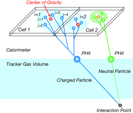
Figure 1: Schematics showing the cheated PFA concept. Only two cells in a single sampling layer of the calorimeter are shown to simplify the picture though in practice much more cells are expected to be hit over different sampling layers.

Since the PHit carries the information of its parent track, one-to-one matching between the calorimeter cluster and its corresponding charged particle track in the tracking system is possible. Once matched, we just lock the calorimeter cluster as linked to a charged track and just use the tracker information. Calorimeter clusters with no matching charged tracks are hereafter called neutral PFOs, while all the charged tracks are called charged PFOs regardless of whether there are corresponding calorimeter clusters or not.

It is also important to record the mother-daughter correspondence for particles decayed in a tracking volume so as to estimate their effects on the PFA performance. The mother-daughter correspondence is book-kept together with the other information on the daughter track such as its particle ID, position, and momentum, in a so-called BreakPoint object which is created at the beginning of each track. The information stored in the BreakPoint objects will be used to follow particle decays observed as kinks or V⁰s in the tracking volume and to assign correct particle masses to charged PFOs. This book-keeping comprises the major role of the history keeper.

2.b Infinite Calorimeter Segmentation

For a realistic calorimeter design, the granularity of the calorimeter, or equivalently the cell size, is finite and hence the signals created by shower particles stemming from different parent particles sometimes merge into a single hit degrading the cluster separation capability. In order to investigate to what extent this limits the PFA performance, we need to know the performance expected for perfect cluster separation. It is, however, impracticable to implement infinitely fine segmentation even in a Monte Carlo detector simulator. In order to overcome this drawback, we exploit the following trick.

In each hit cell, say cell $i$, we separately store the energy sum of hits originating from the same PHit:

$$E^{c}_{i} = \sum_{j}\,E_{i,j}$$

and their center of gravity:

$$\mbox{\boldmath$\bf x$}^{c}_{i} = \sum_{j}\,E_{i,j}\,\mbox{\boldmath$\bf x$}_{i,j}\,/\,E^{c}_{i},$$

instead of using the cell center as the hit position. In the above expression $E_{i,j}$ and $\mbox{\boldmath$\bf x$}_{i,j}$ are the energy deposit and the position of $j$-th hit in cell $i$ with the same PHit. Denoting the total energy of the cluster originating from the same PHit by

$$E^{c} = \sum_{i}\,E^{c}_{i},$$

we can then calculate its cluster center as

$$\mbox{\boldmath$\bf x$}^{c} = \sum_{i}\,E^{c}_{i}\,\mbox{\boldmath$\bf x$}^{c}_{i}\,/\,E^{c}~{}~{}=~{}~{}\sum_{i}\sum_{j}\,E_{i,j}\,\mbox{\boldmath$\bf x$}_{i,j}\,/\,\sum_{i}\,\sum_{j}\,E_{i,j},$$

showing that the center of gravity calculated this way precisely coincides the one would-be obtained when the segmentation is infinitely fine. It should be also emphasized here that hits from different PHits make multiple centers of gravity in the same cell, which can be later separated even though they are in the same cell, thereby realizing the infinite segmentation in effect.

3 Tool Design

Before coding our tool for history keeping, we set the following guideline to fulfill the required functionality discussed in the last section: a) there must be a versatile mechanism to register user-defined physical volumes whose specified boundaries can be used to define a PHit that marks the source point of a particle shower, b) whether a track is allowed to create a PHit or not depends on whether the track originates from any pre-created PHit or not, which should be checked on a track-by-track basis at the beginning of its tracking, c) the history keeping is to be done on the track-by-track basis by creating a BreakPoint object at the beginning of each track if there is no PHit from which the track stems, and d) the history keeping should be realized making maximum use of existing Geant4 facilities within the framework of JUPITER, e) JUPITER should produce Monte-Carlo truths (i.e. exact hits) and their smearing should be done later in SATELLITES as needed.

The following is a sketch of the tool design we adopted according to the guideline:

1. The history keeping is to be done on the track-by-track basis using J4TrackingAction that inherits from G4UserTrackingAction. Its PreUserTrackingAction method is hence called at the beginning of a new track. The PreUserTracingAction method serially invokes PreTrackDoIt method of each offspring of J4VSubTrackingAction pre-registered to the J4TrackingAction object. Likewise, its Clear method serially invokes Clear method of individual offsprings of J4VSubTrackingAction.

2. J4VSubTrackingAction is an abstract class that serves as a base class for user-defined sub-actions taken by J4TrackingAction thereby extending the G4UserTrackingAction functionality. It has a method called Clear to reset the object state.

3. J4HistoryKeeper is implemented as a derived class from J4VSubTrackingAction and, in its PreTrackDoIt method, scans through a collection of pre-registered J4PHitKeeper objects corresponding to a collection of bounding surfaces. It then creates a J4BreakPoint object if none of them has been hit by any ancestors of the new track,

4. J4PHitKeeper also inherits from J4VSubTrackingAction. Its PreTrackDoIT method checks if this new track is stemming from any pre-created PHit, and, if not, resets its sate to allow creation of a new PHit. When its corresponding boundary is hit by the current track, a PHit object is created, if it is allowed, to tag subsequent daughter tracks possibly created in a shower.

3.a Extension of G4UserTrackingAction

The G4UserTrackingAction class provides one with a handy tool to perform a user-defined action on a track-by-track basis. In its original form, however, it allows only a single action. In order to extend its functionality to accept multiple user-defined actions, we have introduced the concept of SubTrackingAction as sketched above.

J4VSubTrackingAction

The abstract base class J4VSubTrackingAction has the following methods:

void PreTrackDoIt(const G4Track *aTrack = 0) = 0 
which is pure virtual and to be implemented by its derived class to take a sub-tracking action for the given track.

void Clear() 
which does nothing, and to be overridden in the derived class as needed.

This class just specifies the interface and requires its users to implement the methods listed above.

J4TrackingAction

The J4TrackingAction class is a singleton inheriting from G4UserTrackingAction. It has, among others, an STL vector as a data member to store pointers to objects derived from the J4VSubTrackingAction class. Its major methods include the following:

static J4TrackingAction *GetInstance() 
which returns the pointer to the single instance of J4TrackingAction.

void Add(J4VSubTrackingAction *stap) 
which registers a user-defined object derived from J4VSubTrackingAction. When *stap has already been registered, the pre-registered one is erased and the new entry is appended.

void PreUserTrackingAction(const G4Track *aTrack) 
which loops over the registered offsprings of J4VSubTrackingAction and invokes their PreTrackDoIt methods.

void Clear() 
which loops over the registered offsprings of J4VSubTrackingAction and invokes their Clear methods.

3.b P-Hits and P-Hit Keeper

A PHit is a generic name for a Pre-Hit or a Post-Hit, which stands for a virtual hit created on a boundary of a G4PhysicalVolume beyond which particle showering is expected. The PHit creation is done in the user-overridden ProcessHits method of a user-defined virtual detector derived from G4SensitiveDetector corresponding to the physical volume. Notice that PHits are created for all kinds of particles, even neutrinos, that pass through the boundary. One PHit class is defined inheriting from the J4VTrackHit class for each such boundary. The J4VTrackHit class carries basic track hit information such as track ID, particle ID, position, momentum, TOF, energy deposit, etc. and setters and getters to access them. An individual PHit class has a data member to store PHit ID and a static data member to store the current PHit ID, which can be retrieved by a static method to mark calorimeter hits as needed.

J4PHitKeeper

The J4PHitKeeper class inherits from J4VSubTrackingAction. It serves as a base class for a PHitKeeper class defined for an individual PHit class corresponding to a boundary beyond which particle showering is expected. The J4PHitKeeper class has data members to store i) the current incident track ID (fInTrackID) that is expected to create or has already created a PHit, ii) the track ID (fTopTrackID) of the next track to be processed, if any, after the offsprings from the PHit are exhausted, and iii) a flag (fIsPHitCreated) to tell whether a PHit has been created or not. The major methods of J4PHitKeeper are listed below:

void PreTrackDoIt(const G4Track *) 
implements the corresponding base class pure virtual method so as to reset fInTrackID and fTopTrackID to INT_MAX and fIsPHitCreated to FALSE upon encountering a new track which has a track ID smaller than fTopTrackID.

G4bool IsNext() 
returns FALSE if a PHit has already been created. If not, it updates fInTrackID and fTopTrackID and returns TRUE to tell the caller (the ProcessHit method of the sensitive detector defining the virtual boundary) that a new PHit is to be created.

void Reset(G4int k = INT_MAX) 
resets fInTrackID and fTopTrackID to k.

G4bool IsPHitCreated() 
returns fIsPHitCreated, which is TRUE if a PHit has been created, and FALSE otherwise.

The algorithm of J4PHitKeepr heavily depends on Geant4’s default track stacking scheme, which is worth explaining here for readers unfamiliar to it. By default Geant4 uses two types of track stacks, a Primary Stack (PS) and a Secondary Stack (SS).

At the beginning of each event, primary particles $1,\cdots,n$ are pushed into PS. According to the ”last in first out” rule, the top entry, track $n$, is popped out for tracking. Notice that there remains $n-1$ tracks in PS at this point. All the secondary particles produced while track $n$ is being processed are pushed into SS. Let us assume that there will be $m$ secondary particles stacked into SS by the time track $n$ is disposed of. All of these $m$ secondary particles in SS are moved to PS upon the death of track $n$ and numbered serially as track $n+1,\cdots,n+m$. Notice that there are $n+m-1$ tracks in PS at this point since track $n$ has been popped out and disposed of.

The key point is to bookmark the secondary track which is to be created just after the creation of a PHit by the track which has been being processed, track $n$ in the present case. The track ID with the bookmark will be ${\tt fTopTrackID}=n+k^{\prime}+1$ where $k^{\prime}(\leq m)$ is the number of secondary particles in SS at the time of the PHit creation. Further PHit creation is to be forbidden until it becomes necessary.

The top of the stack, track $n+m$, is popped out and to be processed as before. Track $n+m$ will produce further $m^{\prime}$ secondary particles to be pushed into PS upon its death and to be numbered as track $n+m+1,\cdots,n+m+m^{\prime}$.

This procedure is repeated and after some time all the secondary particles originating from the track created the last PHit will be disposed of and the next track to be popped out from PS will have a track ID that is smaller than that of the last bookmarked one, fTopTrackID. This signals a new incident track which is allowed to create a new PHit. By repeating this procedure until all the tracks in PS are exhausted, we can mark all the calorimeter hits with corresponding PHits.

3.c Break Points and History Keeper

The purpose of the history keeper is to allow us to trace back to kink and V⁰ particles that decay before entering calorimeters so as to correctly link clusters to tracks. As sketched above, the history keeper is implemented as a J4VSubTrackingAction so as to create a J4BreakPoint object for each new track until a PHit is created on any of the pre-registered boundaries beyond which particle-shwering is expected.

J4BreakPoint

The J4BreakPoint class has data members to store the information about a track at its starting position such as track ID (fTrackID), parent track ID (fParentID), charge, particle ID, time, position, 4-momentum, etc.. In addition it has a static data member called fgBreakPointMap, which is an STL map that links track ID to a J4BreakPoint object. Besides the getters to these data members, J4BreakPoint has the methods listed below:

static J4BreakPoint *GetBreakPoint(G4int trackID) 
returns the pointer to the J4BreakPoint object corresponding trackID.

static void Clear() 
clears the track-to-break-point map.

J4HistoryKeeper

The J4HistoryKeeper class is a singleton that inherits from J4VSubTrackingAction. It has an STL vector (fPHitKeepers) as a data member to store registered J4PHitKeepers that correspond to boundaries beyond which particle-showering is expected. As sketched above, it scans through these pre-registered J4PHitKeeper objects to make sure that none of them has a PHit, and then creates a J4BreakPoint object. The major methods of J4HistoryKeeper are listed below:

static J4HistoryKeeper *GetInstance() 
returns the pointer to the single instance of J4HistoryKeeper.

void PreTrackDoIt(const G4Track *) 
implements the corresponding base class pure virtual method. It scans through the pre-registered J4PHitKeeper objects in fPHitKeepers to make sure that none of them has a PHit by calling their IsPHitCreated() method. It then creates a J4BreakPoint object.

void Cleart() 
calles J4BreakPoint::Clear().

void SetPHitKeeperPtr(J4PHitKeeper *phkp) 
pushes back the input J4PHitKeeper pointer into fPHitKeepers.

S4BreakPoint

Upon the completion of Monte Carlo truth generation by JUPITER, each J4BreakPoint object is copied to its SATELLITE dual, an S4BreakPoint object. The S4BreakPoint object inherits from ROOT’s TObjArray and stores pointers to its daughter S4BreakPoints, if any. It has additional methods such as

void LockAllDescendants() 
which flags all of its descendants as locked. This functionality proves handy to avoid double counting of energies.

TObject *GetPFOPtr() 
which returns the pointer to its corresponding Particle Flow Object (PFO), if any.

void SetPFOPtr(TObject *pfop) 
which is the setter corresponding to GetPFOPtr to be invoked from a PFO maker.

4 Tool Usage

What a tool user has to do for the history keeping is as follows:

• Inheriting G4SensitiveDetector, create a sensitive detector class, say J4XXSD, that corresponds to a boundary on which a PHit object (J4XXPHit) is to be created for each particle that is expected to produce a shower beyond that boundary.

• Inheriting J4PHitKeeper, create a J4XXPHitKeeper as a singleton to bookkeep J4XXPHits.

• In J4XXSD’s constructor, do

  Ψ  J4XXPHitKeeper *phkp = J4XXPHitKeeper::GetInstance();
  Ψ  J4TrackingAction::GetInstance()->Add(phkp);
  Ψ  J4TrackingAction::GetInstance()->Add(J4HistoryKeeper::GetInstance());
  Ψ  J4HistoryKeeper::GetInstance()->SetPHitKeeperPtr(phkp);
  

  in order to register the J4XXPHitKeeper to J4TrackingAction and to J4HistoryKeeper.

• In J4XXSD’s ProcessHits($\cdots$) method, do

  Ψ  if (J4XXPHitKeeper::GetInstance()->IsNext()) {
  ΨΨ  // create and store a J4XXPHit object
  Ψ  }
  

• In ProcessHits($\cdots$) of each calorimeter sensitive detector, which usually corresponds to a single calorimeter cell, store the centers of gravity and energy deposits of particles from different PHits as different calorimeter hits even in the same cell and mark them with the current PHit ID obtainable from an appropriate J4PHitKeeper object.

This ensures the history keeping to be continued until any one of the pre-registered boundaries is hit and beyond which the calorimeter hits are marked with the PHit ID put to the PHit created on that boundary.

The PHit and BreakPoint information can be used in SATELLITES to perform the CPFA as well as to decompose the various factors contributing to the jet energy resolution as we will see later.

5 Application to Studies of Fundamental Limits on the PFA Performance

Various factors may affect the PFA performance. The following is a list of possible contributors to the jet energy resolution:

• calorimeter resolution and acceptance,

• tracker resolution and acceptance,

• kink and V⁰ influence,

• effects of missing energies due to neutrinos,

• effects of particle ID and mass assignment.

In this section we will investigate how significant these factors are, making full use of the tool we described so far.

5.a Detector Model

As shown in Fig.2 (left) the detector model we use in this paper features a Time Projection Chamber (TPC) as its central tracker and a lead-scintillator-sandwich-type calorimeter (CAL) with a tower geometry pointing to the interaction point, both of them installed inside a $3\,$T super-conducting solenoidal magnet (SOL) with a bore radius of $3.75\,$m and a half length of $4.75\,$m. The SOL is surrounded by a muon detector that also serves as a return yoke for the magnetic field. The detector model also incorporates a vertex detector (VTX) consisting of six layers of silicon pixel detectors and an inner tracker (IT) comprises four cylindrical and seven end-cap layers at each end of silicon detectors.

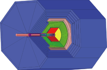
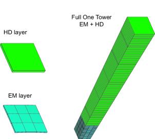
Figure 2: Detector model (left), a calorimeter tower (right) used in this study

The TPC has inner and outer radii of $45$ and $200\,{\rm cm}$, respectively, and is $5.2\,{\rm m}$ long. The tracking system provides a momentum resolution of $\sigma_{p_{T}}/p_{T}=1\times 10^{-4}p_{T}\,[{\rm GeV/c}]$ with the TPC alone, which can be improved by a factor of about two when combined with the IT and VTX.

The inner radius of the barrel part of CAL is $2.1\,{\rm m}$ while the front face of its endcap part is at $2.7\,{\rm m}$ away from the interaction point. As shown in Fig.2 (right) each CAL tower has two sections: electromagnetic (EM) calorimeter section made of 38 layers of $4\,$mm thick lead radiator plate and $1\,$mm thick scintillator tile pairs corresponding to $27.1$ radiation lengths, and hadron (HD) calorimeter section made of 130 layers of $8\,$mm thick lead plate and $2\,$mm thick scintillator tile pairs that follow the EM section. Altogether the single tower has a tower height of $150\,$cm corresponding to more than 6 interaction lengths. The calorimeter provides energy resolutions (stochastic) of $\sigma_{E}/E\simeq 0.15/\sqrt{E\,[{\rm GeV}]}$ for electromagnetic showers and $\sigma_{E}/E\simeq 0.43/\sqrt{E\,[{\rm GeV}]}$ for hadron showers. The single tower has a cross section of about $12\,$cm$\times 12\,$cm at the front face which is subdivided into $3\times 3=9$ columns in the EM section. These finite cell sizes, however, do not affect the CPFA results we show below, since the CPFA effectively realizes infinitely fine segmentation. The model detector system described here has been implemented in JUPITER with Geant4.8.2p01.

Notice that the calorimeter geometry we adopted here differs from the GLD design[9] having a dodecagonal shape and sampling layers parallel to the beam axis in the barrel part and perpendicular to the beam axis in the end-cap parts. This is to avoid the polar angle dependence of the calorimeter resolution due to the variation of the effective sampling thickness, thereby enabling us to access the best attainable PFA performance.

5.b Monte Carlo Data Sample

We have used PYTHIA version 6.319 to generate 4-momenta of final-state particles for the $e^{+}e^{-}\to q\bar{q}$, the $e^{+}e^{-}\to Z^{0}Z^{0}$, and the $e^{+}e^{-}\to Z^{0}H^{0}$ processes. For $e^{+}e^{-}\to q\bar{q}$ and $Z^{0}Z^{0}$ events we restrict final-state quark flavors to $u$, $d$, and $s$ to minimize the effects of neutrinos and the initial state radiation (ISR) switched off to avoid the effect of ISR photons escaping into the beam-pipe. Switching off ISR is important in particular at higher energies, since otherwise the radiative return to $Z^{0}$: $e^{+}e^{-}\to\gamma Z^{0}\to\gamma+q\bar{q}$ would dominate the cross section. For the $e^{+}e^{-}\to Z^{0}Z^{0}$ events we have set the $Z^{0}$ natural width to zero and one $Z^{0}$ is forced to decay into $\nu\bar{\nu}$ so that the apparent resolution of the reconstructed $Z^{0}$ mass is affected neither by the natural width nor by confusions in jet clustering. At a given energy point we have generated 10k events of each process and the 4-momenta of the final-state particles have been fed into JUPITER in the HEPEVT format and processed through the detector model described above using a Geant4 physics list that implements various interactions in the detector materials such as multiple scattering, energy loss, electromagnetic showering, hadronic interactions, etc.. Fig.3 shows a typical $Z^{o}$ pole event simulated this way.

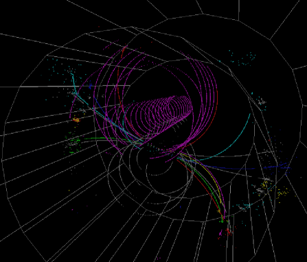
Figure 3: A typical $Z^{0}\to q\bar{q}$ event.

In the figure, calorimeter hits belonging to the same shower cluster due to the same parent particle are drawn in the same color using PHit information. We can see a clear correspondence between a cluster and its parent charged track for a charged PFO.

As basic selection cuts we require, in the following, the number of PFOs in a jet to be 5 or more and the absolute value of the cosine of its polar angle to be less than 0.8, unless otherwise stated.

5.c Analysis Methods

In what follows we will use two analysis methods to estimate the size of contributions from various factors to the PFA performance. The first method directly compares the measured energy and corresponding MC truth on an event-by-event basis and hence is very clear cut but cannot be applied to the jet invariant mass resolution. The second method relies on an assumption about the statistical independence of various factors contributing to the jet energy or jet invariant mass resolutions. It is indirect but allows us to decompose various contributions not only to the jet energy resolution but also to the jet invariant mass resolution.

5.c.1 Direct Method

The first method starts from the following energy sum rule that holds on an event-by-event basis:

$$E^{\rm true}_{\rm CM} = E^{\rm true}_{\rm tk}+E^{\rm true}_{\rm EM}+E^{\rm true}_{\rm HD}+E^{\rm true}_{\nu\,\&\,{\rm AH}}$$ (5.1)

$$= (E^{\rm meas}_{\rm tk}-\Delta E_{\rm tk})+(E^{\rm meas}_{\rm EM}-\Delta E_{\rm EM})+(E^{\rm meas}_{\rm HD}-\Delta E_{\rm HD})+E^{\rm true}_{\nu\,\&\,{\rm AH}}$$ (5.2)

$$= E^{\rm meas}_{\rm CM}-\Delta E_{\rm tk}-\Delta E_{\rm EM}-\Delta E_{\rm HD}+E^{\rm true}_{\nu\,\&\,{\rm AH}},$$

where $E^{\rm meas/true}_{\rm tk}$, $E^{\rm meas/true}_{\rm EM}$, and $E^{\rm meas/true}_{\rm HD}$ are the measured/true energy sum of charged tracks, photons, and neutral hadrons, respectively and $E^{\rm true}_{\nu\,\&\,AH}$ is the undetected energy due to neutrinos and the acceptance holes of the detector. By looking at the distribution of the measurement errors for each component and fitting a Gaussian to it, we can estimate the contribution from that component to the jet energy resolution. For the Gaussian fitting we iteratively adjust the fit range so that the fit range would correspond to 2 $\sigma$s.

5.c.2 Indirect Method

The first method implies that

$$\sigma_{E_{\rm CM}}^{2} = \left<(E^{\rm meas}_{\rm CM}-E^{\rm true}_{\rm CM})^{2}\right>$$ (5.3)

$$= \left<(\Delta E_{\rm tk})^{2}\right>+\left<(\Delta E_{\rm EM})^{2}\right>+\left<(\Delta E_{\rm HD})^{2}\right>+\left<(E^{\rm true}_{\nu\,\&\,{\rm AH}})^{2}\right>$$ (5.4)

$$= \sigma_{E,\,\rm tk}^{2}+\sigma_{E,\,\rm HD}^{2}+\sigma_{E,\,\rm others}^{2}+\sigma_{E,\,\rm others}^{2},$$

provided that the measurement errors as well as the undetected energy are mutually statistically independent. In the second method, we assume that this holds generically for both the jet energy and the jet invariant mass resolutions:

$$\sigma^{2} = \sigma_{\rm tk}^{2}+\sigma_{\rm EM}^{2}+\sigma_{\rm HD}^{2}+\sigma_{\rm others}^{2},$$

where $\sigma_{\rm tk}^{2}$, $\sigma_{\rm EM}^{2}$, $\sigma_{\rm HD}^{2}$, and $\sigma_{\rm others}^{2}$ are the contributions from the detector resolutions for charged tracks, photons, neutral hadrons, and various other effects, respectively. If we want to estimate $\sigma_{\rm EM}^{2}$, for instance, we replace the measured photon energies with their corresponding true values obtained from the history keeper. Then the resultant resolution will be

$$\sigma_{\rm EM=exact}^{2} = \sigma_{\rm tk}^{2}+\sigma_{\rm HD}^{2}+\sigma_{\rm others}^{2},$$

since the contribution to the resolution from the measurement errors for photons ($\sigma_{\rm EM}^{2}$) should vanish then. We can hence obtain $\sigma_{\rm EM}^{2}$ as

$$\sigma_{\rm EM}^{2} = \sigma^{2}-\sigma_{\rm EM=exact}^{2}.$$

We will use this method repeatedly to decompose the jet invariant mass resolution into various factors.

5.d $e^{+}e^{-}\to q\bar{q}$ Events

5.d.1 Performance on the $Z^{0}$ pole

We start from the treatment of kink particles such as $K^{\pm}$s and $\pi^{\pm}$s that decay in the tracking system. A kink has a mother track and its charged and neutral daughters in general. For instance a kink from the $K^{\pm}\to\pi^{\pm}\,\pi^{0}$ decay may yield a daughter $\pi^{\pm}$ track and two neutral clusters from the $\pi^{0}\to\gamma\gamma$ decay. In this case, we have one charged PFO for the parent $K^{\pm}$ track, one charged PFO for the daughter $\pi^{\pm}$ track, and two neutral PFOs for the daughter $\gamma$s from the $\pi^{0}$ decay. In practice there are three approaches we can take here:

• No kink treatment: If we don’t care about the kink all of these PFOs will be used in the jet reconstruction and the energy will be double counted.

• Kink daughter scheme: To avoid the double counting, we may use just kink daughters throwing away the kink mother.

• Kink mother scheme: We use the kink mother throwing away the charged kink daughter. The neutral kink daughters will be be double counted in this case.

The kink mother scheme turns out to give the best resolution (30% improvement as compared to the no kink treatment case) as shown in Figs.4 a) through c)

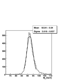
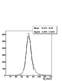
Figure 4: Comparison of reconstructed $Z^{0}$ mass distributions in the three schemes for kink treatment: a) no kink treatment, b) kink daughter scheme, and c) kink mother scheme.

in spite of the risk of energy double counting. This is because of the dominance of $K^{\pm}\to\mu^{\pm}\nu$ decay where the neutral daughter escapes detection. In what follows we will use the kink mother scheme.

If incorrectly treated, the V⁰s such as $\gamma$s converted into $e^{+}e^{-}$ pairs, $K^{0}_{S}$s, and $\Lambda^{0}$s might also affect the jet invariant mass measurements, since their momenta would be wrongly reconstructed. In order to investigate this effect, let us take a look at the $Z^{0}$ mass distributions with and without a V⁰ finder relying on Monte Carlo truth from the history keeper: when a pair of charged tracks in the tracking system is found to be coming from a V⁰, we re-evaluate the reconstructed daughter momenta at its decay vertex to reconstruct the V⁰ momentum.

The effect of the V⁰ treatment on the $Z^{0}$ mass resolution, however, turned out to be less significant than the effect of kink treatments as shown in Figs. 5 a) and b).

Figure 5: Comparison of reconstructed $Z^{0}$ mass distributions (a) with and (b) without the V⁰ finder explained in the text.

This can be attributed to the fact that for a high momentum V⁰ the relative error in the sum of the reconstructed momenta of the V⁰ daughters is expected to be small since their opening angle becomes large only when one of them has a negligible momentum. Besides, the V⁰ treatment does not affect the total energy of the system unlike the kink treatments. Although the effect is small we apply the V⁰ treatment in what follows for completeness.

With the kinks and V⁰s treated we can now investigate the effects of the detector resolutions on the jet invariant mass measurements. Fig. 6 a) shows the $Z^{0}$ mass distribution with the 4-momenta of PFOs corresponding to neutral electromagnetic PFOs (photons, electrons, or positrons with no associated tracks) replaced by the MC truths.

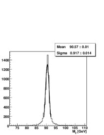
Figure 6: Comparison of reconstructed $Z^{0}$ mass distributions with the 4-momenta of PFOs replaced by MC truths for (a) electromagnetic showers with no associated tracks, (b) both electromagnetic and hadron showers with no associated tracks, and (c) all of them.

The resolution difference between this and Fig. 5 a) hence represents the contribution of the calorimeter resolution for electromagnetic showers due mostly to photons from $\pi^{0}$s: $\sqrt{2.20^{2}-1.96^{2}}=1.02\,$GeV ((1.02/2.20)²=21%).

Further replacing the 4-momenta of PFOs corresponding to hadrons with no associated tracks by the MC truths from the history keeper, we have Fig. 6 b). The difference between Figs. 6 a) and b) gives the contribution from the calorimeter resolution for hadron showers: $\sqrt{1.96^{2}-0.917^{2}}=1.73\,$GeV (62%).

In order to estimate the contribution from the tracker resolution, we switch off the tracker resolution in Fig. 6 c) by replacing the 4-momenta of the charged PFOs with the corresponding MC truths from the history keeper. The resultant difference between Figs. 6 b) and c) yields the contribution from the tracker resolution: $\sqrt{0.917^{2}-0.829^{2}}=0.39\,$GeV (3%).

The remaining $0.829\,$GeV (14%) must be coming from the effects of undetected particles due to acceptance holes or neutrinos, energy double counting, particle misidentification, etc.. Since the undetected particles only make a tail on the lower mass side of the peak, the tail on the higher mass side suggests some double counting of energy due for instance to the effect of neutral kink daughters discussed above or the effect of incorrectly included mass energies of particles kicked out from detector materials. To study these effects, let us now switch to the direct method. Fig. 7 a) shows the visible energy distribution for the same sample of PFOs as used for the mass distribution in Fig. 5 a).

Figure 7: Visible energy distributions: (a) that corresponding to the mass distribution in Fig. 5 a), (b) that with the double counted daughter energies avoided by using the history keeper, and (c) the same as (b) but the 4-momenta of PFOs replaced by the MC truths as in Fig. 6 c).

The visible energy distribution is almost identical to the mass distribution as expected. On the other hand, Fig. 7 b) is the same distribution with the double counted daughter energies eliminated by using the history keeper. The difference of the two gives the contribution from the double counting: $\sqrt{2.20^{2}-2.01^{2}}=0.92\,$GeV (17%). Notice that this includes the contribution from the finite detector resolutions for the double counted energies. The contribution from the double counted energies alone can be obtained from the difference between Figs. 6 c) and 7 c): $\sqrt{0.829^{2}-0.698^{2}}=0.45\,$GeV (4%). As seen in 7 c), the distribution still has a higher tail indicating that there still remains some contribution from energy overestimation due to the mass energies of particles kicked out from the detector materials.

To see their contributions more clearly we plot the exact values of the double counted energies and the exact values of undetected energies (with an overall minus sign) in Figs. 8 a) and b), respectively.

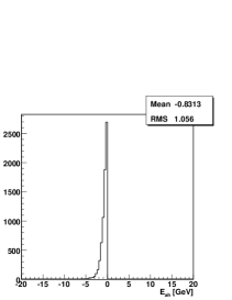
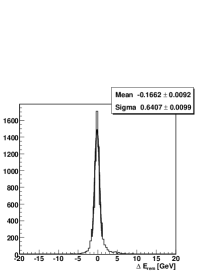
Figure 8: Distributions of (a) the true event-by-event sum of double counted energies, (b) the true event-by-event sum of undetected energies with an overall minus sign, and (c) the event-by-event sum of (a) and (b).

As expected, the double counted energies have only a higher tail while the undetected energies have only a lower tail, thereby resulting in a more or less symmetric distribution for their sum as shown in Fig. 8 c). Since we restrict the $Z^{0}$ decays only to $u$, $d$, and $s$ quarks, the effect of neutrinos is negligible and the undetected energy in Fig. 8 b) is mostly due to acceptance holes: $p_{T}$ cutoff of about $0.23\,$GeV for charged particles from the IP and the forward and the backward regions near the beam pipe (see Fig. 9).

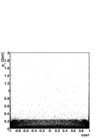
Figure 9: Distribution of $(\cos\theta,p_{T})$ of undetected primary particles on the $Z^{0}$ pole.

With the effect of the double counting eliminated, we can now break up the contributions to the jet energy resolution from detector resolutions on an event-by-event basis using the history keeper. Figs. 10 a) through c) plot the differences of the reconstructed energies from their corresponding MC truths for the charged PFOs, the neutral electromagnetic PFOs, and the neutral hadronic PFOs, respectively. Notice that as the MC truths we use the energies of primary particles to ensure that their sum to have a $\delta$-function-like distribution centered at $E_{\rm CM}=91.18\,$GeV.

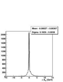
Figure 10: Distributions of the difference of the total reconstructed energies from the corresponding MC truths for (a) charged PFOs, (b) neutral PFOs with electromagnetic showers, and (c) neutral PFOs with hadron showers.

The measurement error distribution for the charged PFOs has a sharp peak with a rather broad component beneath it. Since we are comparing the measured charged track energies with those of their corresponding primary particles, the reconstructed energies can be significantly lower than those expected from the detector resolution when some secondary particles are left undetected as in the case of kink tracks or when the $dE/dx$ contribution is non-negligible. On the other hand, the energies of some secondary charged particles kicked out from the detector materials, protons in particular, can be overestimated if the mass energies are included. These two effects explain the broad component. By the same token, the apparent resolutions are worse than those expected from the detector performance also for the neutral PFOs. One can also notice a sharp peak at zero in Fig. 10 c). This is due to events in which there is no detected neutral hadrons.

Figs. 10 a) through c) tell us the contributions from (a) the tracker resolution ($\sigma_{\rm tk}=0.2\,$GeV: narrow component only), (b) the calorimeter resolution for electromagnetic showers ($\sigma_{\rm EM}=0.85\,$GeV), and (c) the calorimeter resolution for hadronic showers ($\sigma_{\rm HD}=1.52\,$GeV). These values can be compared with the previous values obtained with the indirect method: $\sigma_{\rm tk}=0.39\,$GeV, $\sigma_{\rm EM}=1.02\,$GeV, and $\sigma_{\rm HD}=1.73\,$GeV. Considering the energy double counting in the previous values, the agreement is reasonable.

Fig. 11 a) shows the decomposition of the true visible energy into the three components corresponding to those shown in Figs. 10 a) through c).

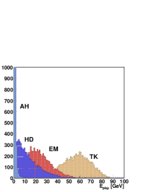
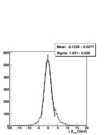
Figure 11: (a) MC truths for the energy sum distributions for charged (TK), neutral electromagnetic (EM), and neutral hadronic (HD) PFOs corresponding to Figs. 10 a) through c), and undetected primary particles due to acceptance holes (AH); (b) the measurement error in the total visible energy corresponding to the sum of these three.

On the average, the charged, the neutral electromagnetic, and the neutral hadronic PFOs share $56.2$, $22.6$, and $11.6\,$GeV of the center of mass energy on the $Z^{0}$ pole. Ignoring the constant terms in the calorimeter resolutions, we can relate these average energies to the resolution contribution:

$$\sigma_{E}^{2} = \frac{1}{N_{\rm evt}}\,\sum_{i=1}^{N_{\rm evt}}\,\frac{1}{N_{{\rm tk},i}}\,\sum_{j\in{\rm tk}}\,\sigma_{j}^{2}+\frac{1}{N_{\rm evt}}\,\sum_{i=1}^{N_{\rm evt}}\,\frac{1}{N_{{\rm EM},i}}\,\sum_{j\in{\rm EM}}\,\sigma_{j}^{2}+\frac{1}{N_{\rm evt}}\,\sum_{i=1}^{N_{\rm evt}}\,\frac{1}{N_{{\rm HD},i}}\,\sum_{j\in{\rm HD}}\,\sigma_{j}^{2}$$ (5.5)

$$\simeq \sigma_{\rm tk}^{2}+\frac{1}{N_{\rm evt}}\,\sum_{i~{}1}^{N_{\rm evt}}\,\frac{1}{N_{{\rm EM},i}}\,\sum_{j\in{\rm EM}}\,(0.15\times\sqrt{E_{j}})^{2}+\frac{1}{N_{\rm evt}}\,\sum_{i~{}1}^{N_{\rm evt}}\,\frac{1}{N_{{\rm HD},i}}\,\sum_{j\in{\rm HD}}\,(0.43\times\sqrt{E_{j}})^{2}$$ (5.6)

$$= \sigma_{\rm tk}^{2}+(0.15)^{2}\times\left<E_{\rm EM}\right>+(0.43)^{2}\times\left<E_{\rm HD}\right>~{}=~{}\sigma_{\rm tk}^{2}+\sigma_{\rm EM}^{2}+\sigma_{\rm HD}^{2}.$$

This gives the following estimates for the contributions from the detector resolutions: $\sigma_{\rm EM}=0.15\times\sqrt{22.6}=0.71\,$GeV and $\sigma_{\rm HD}=0.43\times\sqrt{11.6}=1.46\,$GeV. These values are significantly smaller than those obtained from Figs. 10 b) and c). As pointed out above, this is because the measurement errors are defined as the differences between the measured PFO energies and those of the corresponding primary particles, which sometimes decay before making those PFOs. In order to confirm this we have looked at the difference between the measured PFO energies and the MC truths for the directly corresponding particles and found: $\sigma_{\rm EM}=0.70\,$GeV and $\sigma_{\rm HD}=1.41\,$GeV, being in good agreement with the above estimates. Fig. 11 b) shows the distribution of the sum of the contributions from the three components. The total detector resolution contribution of $\sigma_{\rm det}=1.83\,$GeV is consistent with the quardratic sum: $\sigma_{\rm det}=\sqrt{0.39^{2}({\rm tk})+0.85^{2}({\rm EM})+1.52^{2}({\rm HD})}=1.78\,$GeV, when we assume $\sigma_{\rm tk}=0.39\,$GeV instead of $0.20\,$GeV taken into account the broad component. This confirms the statistical independence of the resolution contributions from the different detectors as expected.

5.d.2 Energy Dependence

The next question is how the jet energy resolution depends on the energy. Fig. 12 plots the energy resolutions normalized by the square root of the center of mass energies for $E_{\rm CM}=$91.18, 200, 350, 500 GeV.

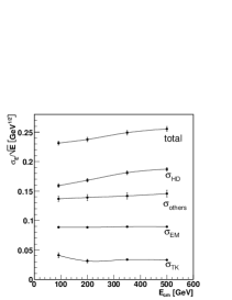
Figure 12: Energy dependence of the energy resolutions normalized by the square root of the center of mass energies. The smooth curves in the figure are drawn just to guide eyes.

From the bottom to the top, the lines correspond to the contribution from the charged PFOs ($\sigma_{\rm tk}$), that from the acceptance hole, neutrinos, and the energy double counting ($\sigma_{\rm others}$), that from the neutral electromagnetic PFOs ($\sigma_{\rm EM}$), that from the neutral hadronic PFOs ($\sigma_{\rm HD}$), and the total jet energy resolution. The figure suggests that our model detector would have a jet energy resolution: $\sigma_{E_{\rm jet}}\simeq 0.23\times\sqrt{E_{\rm jet}\,\mbox{[GeV]}}$ with a slight increase with energy. The increase can mostly be attributed to the contribution from the neutral hadronic PFOs. The energy dependence of the contribution from the neutral hadronic PFOs is largely due to our unsophisticated calorimeter calibration with a single conversion factor for each of the electromagnetic and hadronic components. It might hence be reduced by improving the calibration method. As stated earlier, optimization of the calibration method as well as the calorimeter configuration is, however, beyond the scope of this paper.

Notice that the contributions from the calorimeter resolutions are estimated by the direct method, while that from the tracker resolution is by the indirect method here. The remaining contribution ($\sigma_{\rm others}$) hence includes the fluctuation of the double counted energies due to the finite detector resolutions and hence is significantly larger than the remnant contribution we discussed above in examining Fig. 6 c). It is also remarkable that the tracker contribution ($\sigma_{\rm tk}$) too seems to scale approximately as $\sigma_{\rm tk}\propto\sqrt{E_{\rm CM}}$ at least in the energy range considered here. This is because the tracker contribution is estimated by the indirect method in order to take into account the broad component which might as well be dominated by some stochastic processes. As discussed previously, the broad component indeed comes from stochastic processes such as undetected daughter particles or wrongly included mass energies for protons kicked out from the detector materials. This is in contrast to the sharp component that is solely determined by the tracker resolution which roughly scales as $\sigma_{\rm tk,sharp}\simeq 5\times 10^{-4}\left<E_{\rm tk}\right>$, indicating the dominance of relatively low-momentum tracks for which the effect of multiple scattering is significant.

5.e $e^{+}e^{-}\to Z^{0}Z^{0}$ Events

In the previous subsection we have examined how jet energy resolution depends on jet energy. It is practically more important and probably more interesting to examine how the invariant mass resolution of a jet pair from a gauge boson changes with its momentum, since it would determine the $W/Z$ separation capability with their jet invariant mass measurements. In this subsection we will hence look at the invariant mass resolution for the jet pair from a $Z^{0}$ boson decay in the $e^{+}e^{-}\to Z^{0}Z^{0}$ process.

Fig. 13 a) shows the invariant mass distribution at $E_{\rm CM}=700\,{\rm GeV}$ or, equivalently, a $Z^{0}$ energy of $350\,{\rm GeV}$. Here we have relaxed the cut on the absolute value of the cosine of the polar angle of each jet to 0.95 from its default 0.8, since otherwise the acceptance becomes too small (less than $20\%$) due to the forward backward peaks of the $Z^{0}$ boson production angle distribution. Nevertheless the acceptance is significantly smaller (about $40\%$) at $E_{\rm CM}=700\,{\rm GeV}$ than that for the on-pole $Z^{0}$ production.

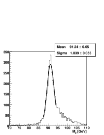
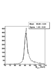
Figure 13: Jet invariant mass distributions for a jet pair from $e^{+}e^{-}\to Z^{0}Z^{0}$ followed by $Z^{0}\to\nu\bar{\nu}$ and $Z^{0}\to q\bar{q}$ (a) that with the standard treatment corresponding to the mass distribution in Fig. 5 a), (b) that with double counted daughter PFOs eliminated by using the history keeper, and (c) the same as (b) but with the undetected primary particles artificially added in.

The figure tells us that, in this highly boosted case, the core part of the distribution has a narrower width than that of $Z^{0}$ bosons at rest, indicating the improvement of the relative error ($\sigma_{E}/E$) with energy, while there is a significant tail towards the higher mass region. The Gaussian fit range is changed here to $(-2,+1.5)$-$\sigma$s so as to avoid the higher tail affecting the fit. By eliminating the double counted daughter PFOs using MC truths, we can suppress the higher tail to some extent as shown in Fig. 13 b) but not completely. In order to see the acceptance hole effect we plot the mass distribution in Fig. 13 c) with the undetected primary particles artificially added in. The width of the core part becomes significantly narrower, but the higher tail persists as expected; their addition could only enhance the higher tail but not reduce it.

The origin of the higher tail has been traced to the over-counted mass energies for the charged PFOs corresponding to secondary protons kicked out from the detector materials. As with the secondary neutrons kicked out from the detector materials, the mass energies of these secondary protons should be subtracted.

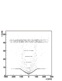
Figure 14: Jet invariant mass distributions for a jet pair from $e^{+}e^{-}\to Z^{0}Z^{0}$ followed by $Z^{0}\to\nu\bar{\nu}$ and $Z^{0}\to q\bar{q}$ (a) that corresponding to the mass distribution in Fig. 13 c), and (b) that corresponding to the mass distribution in Fig. 13 a), but with the mass energies subtracted for secondary protons kicked out from the detector materials. (c) The production points of secondary protons kicked out from the detector materials in the $r$-$z$ view.

Fig. 13 c) becomes Fig. 14 a) after this mass energy subtraction. Fig. 14 c) plots the production points of the secondary protons kicked out from the detector materials, which clearly reflects the material distributions for the beam pipe, the VTX and IT layers and the inner wall of the TPC. Since the production points are so well defined we might be able to separate significant fraction of these secondary protons and subtract their mass energies provided that they are identified as protons by the energy loss measurements in the TPC. Fig. 14 b) is the invariant mass distribution assuming that such mass energy subtraction is practicable. The higher tail is significantly reduced as compared to Fig. 13 a). In what follows, however, we will not apply this mass energy correction.

Fig. 15 plots the invariant mass resolutions, as obtained by the asymmetric Gaussian fits described above, normalized by the square root of the $Z^{0}$ mass $M_{Z}=$91.18 GeV as a function of the $Z^{0}$ momentum.

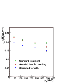
Figure 15: Momentum dependence of the invariant mass resolutions for 2-jet systems from $Z^{0}$ decays normalized by the square root of the $Z^{0}$ mass.

The circles, squares, and reverse triangles are ones with the standard treatment, with the double counting avoided, and with the correction of undetected particle momenta, respectively. The figure shows that the invariant mass resolution indeed improves with the $Z^{0}$ momentum, though it is not as quickly as $1/\sqrt{E_{Z}}$. Denoting the two jet energies by $E_{1}$ and $E_{2}$ and ignoring the individual jet masses, we have an approximate formula for the relative error on the invariant mass of the jet pair:

$$\frac{\sigma_{M}}{M} \simeq \frac{1}{2}\,\sqrt{\left(\frac{\sigma_{E_{1}}}{E_{1}}\right)^{2}+\left(\frac{\sigma_{E_{2}}}{E_{2}}\right)^{2}}~{}\simeq~{}\frac{a}{2}\,\sqrt{\frac{1}{E_{1}}+\frac{1}{E_{2}}},$$

where $a\simeq 0.23\sim 0.25$ as indicated by Fig. 12. This formula tells us that $\sigma_{M}/M$ would scale as $1/\sqrt{E_{Z}}$ if $E_{1}=E_{2}$ but it corresponds to the minimum expected value under the constraint that $E_{1}+E_{2}=E_{Z}=E_{\rm CM}/2$, being consistent with the above observation.

5.f $e^{+}e^{-}\to Z^{0}H^{0}$ Events

As our last example, let us consider one of the most important processes for the ILC experiment that is $e^{+}e^{-}\to Z^{0}H^{0}$ and study the $H^{0}$ reconstruction in its hadronic decays. Again we force $Z^{0}$ to decay into $\nu\bar{\nu}$ so as to avoid the effect of jet clustering, but we impose no restriction on the $H^{0}$ decays. We switch on the initial state radiation and beamstrahlung to see possible complications we would encounter in reality. The $Z^{0}$ and the $H^{0}$ widths are finite now but the effect of their finiteness is negligible, since the $H^{0}$ width can be regarded as zero for the purpose of this analysis and the $Z^{0}$ width only induces a small spread in the otherwise-monochromatic $H^{0}$ energy distribution. Under these conditions we have generated 10k events at $E_{\rm CM}=350\,{\rm GeV}$ with $M_{H}=120\,{\rm GeV}$.

Fig. 16 a) is the difference of the reconstructed final-sate invariant mass from the nominal Higgs mass of $M_{H}=120\,{\rm GeV}$.

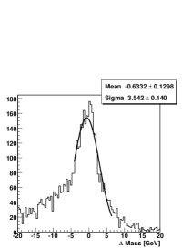
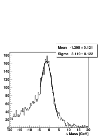
Figure 16: Jet invariant mass distributions for the reconstructed final-state jet systems for $e^{+}e^{-}\to Z^{0}H^{0}$ followed by $Z^{0}\to\nu\bar{\nu}$ (a) that with the standard treatment, (b) that with double counted daughter PFOs eliminated by using the history keeper, and (c) the same as (b) but with the photons from initial state radiations removed.

One can see a huge lower tail there, which is coming mostly from neutrinos from $b$-jet decays as we will see later. To avoid the effect of this huge tail affecting the Gaussian fit, we readjust the fit range here to $(-1,+2)$-$\sigma$s. Nevertheless the resolution, $\sigma_{\Delta M}=3.54\,{\rm GeV}$, is much worse than naive expectaion from the $Z^{0}$ boson cases studied above. Though less dramatic, the higher tail seems also longer than the $Z^{0}$ boson cases. Fig. 16 b) is after eliminating double counted daughter PFOs. The apparent width is reduced significantly to $\sigma_{\Delta M}=3.12\,{\rm GeV}$ ($\sqrt{3.54^{2}-3.12^{2}}=1.67\,$GeV: $(1.67/3.54)^{2}=22\%$ reduction) but both the higher and the lower tails persist. Some significant part of the higher tail turns out to be coming from initial state radiations, which have been switched off artificially for the $Z^{0}$ boson studies presented above. Elimination of photons from the initial state radiations indeed suppresses the higher tail as shown in Fig. 16 c), reducing the sigma value to $\sigma_{\Delta M}=2.90\,$GeV ($\sqrt{3.12^{2}-2.90^{2}}=1.15\,$GeV: 11% reduction).

Let us now examine the neutrino effect. Fig. 17 a) shows the energy distribution of neutrinos from $H^{0}$ decays.

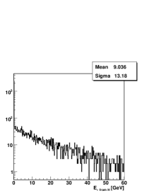
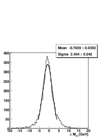
Figure 17: Distributions of (a) energies of neutrinos from $H^{0}$ decays, (b) the same as Fig. 16 c) but 4-momenta of neutrinos from the $H^{0}$ decays artificially added in. (c) the same as (b) but with the other undetected particles also added in.

Using the MC truths from the history keeper, we can add the 4-momenta of these neutrinos and obtain Fig. 17 b). The huge lower tail disappeared as expected and the apparent width now reduces to $\sigma_{\Delta M}=2.40\,$GeV ($\sqrt{2.90^{2}-2.40^{2}}=1.63\,$GeV: 21% reduction). If we further add in the remaining undetected particles escaping into the acceptance holes, we have Fig. 17 c), yielding $\sigma_{\Delta M}=2.19\,$GeV ($\sqrt{2.40^{2}-2.19^{2}}=0.98\,$GeV: 7.7% reduction). This remnant apparent width corresponding to $(2.19/3.54)^{2}=38\%$ of the initial apparent width of Fig. 17 a) and is consistent with that naively expected from the $Z^{0}$ boson result in Fig. 15. Notice also that the mean value of this distribution is consistent with zero.

5.g Fundamental Limitations on the PFA Performance

We have been examining the contributors to the jet energy resolution with the CPFA, taking $e^{+}e^{\to}q\bar{q}$, $Z^{0}Z^{0}$, and $Z^{0}H^{0}$ processes as benchmarks. Let us now summarize the results and discuss their implications from the view point of fundamental limits on the PFA performance. In our on-pole $Z^{0}$ study we have emphasized the importance of appropriate treatment of kinks and demonstrated that the kink mother scheme gives the best resolution in spite of possible energy double counting. If the neutral decay daughters can be identified by testing if their shower axes successfully extrapolate to their corresponding kink positions, the resolution could in principle be further improved by removing such neutral decay daughter PFOs. As compared with the dependence on the kink treatment schemes, the mistreatment of V⁰s turned out to be less harmful, making only a small difference to the jet energy resolution.

Table 1 summaries the contributions from various factors to the jet energy resolution on the $Z^{0}$ pole as estimated with the indirect ($\sigma_{\rm indir}$), the direct ($\sigma_{\rm dir}$), and the detector resolutions for single particles ($\sigma_{\rm det}$).

Table 1: Breakup of the jet energy resolution at the $Z^{0}$ pole into various contributors with the indirect method ($\sigma_{\rm indir}$), that with the direct method using primary break point information ($\sigma_{\rm dir}$), and that expected from single particle detector resolution ($\sigma_{\rm det}$): TK, EM, HD, DC, and AH stand for the charged PFO contribution, that from neutral electromagnetic PFOs, that from neutral hadronic PFOs, that from double counted energies, and that from undetected primary particles due to the acceptance holes of the detector. Notice that the TK contribution obtained with the indirect method (marked by * in the table) is the width of the sharp peak and does not reflect the width of the underlying broad component. For the AH contribution with the direct method the r.m.s. value is shown, since the distribution is far from being Gaussian.

	$\sigma_{\rm indir}$ [GeV]		$\sigma_{\rm dir}[GeV]$	$\sigma_{\rm det}$ [GeV]
TK	0.39	3%	0.19∗	$-$
EM	1.02	21%	0.85	0.70
HD	1.73	62%	1.52	1.46
subtotal	2.05	86%	1.83	$-$
DC	0.45	4%	$-$	$-$
AH	0.70	10%	0.81 (rms)	$-$
total	2.20	100%	2.00	$-$

The detector resolution contributions estimated with the indirect method include those from the fluctuations of the double counted energies. Accordingly, the contribution from the double counted energies of $0.45\,$GeV in the indirect method does not include their fluctuations due to finite detector resolutions. This is the main reason why the indirect method gives larger values than the direct method where the double counting is avoided by locking daughter PFOs. On the other hand the difference between the values obtained with the direct method and the naive estimates from the single particle resolution can be attributed to the fact that the direct method compares the measured PFO energies with the energies of the corresponding primary particles which might decay before detection. Some part of the daughter particles might escape into acceptance holes or some part of the secondary particles might be protons kicked out from the detector materials whose mass energies should have been subtracted.

As we discussed in our $e^{+}e^{-}\to Z^{0}Z^{0}$ study, the effect of the mass energy correction is quite dramatic in particular when the parent $Z^{0}$ is highly boosted. Without the mass energy correction, the reconstructed $Z^{0}$ invariant mass distribution has a significant tail on the higher mass side. Since the production points of the secondary protons from the detector materials show a clear image of the material distribution in the detector, there is a possibility to do this mass energy correction, provided that we can identify protons using, for instance, the energy loss information from the TPC.

With these corrections made, the jet energy resolution can be given by the sum of the contribution from the detector resolutions and the contribution from the undetected particles. Among the detector resolutions the calorimeter resolutions, the HD contribution in particular, dominate obviously. As mentioned earlier we have used a rather unsophisticated calibration method for the calorimeters. It is therefore of prime importance to optimize the calorimeter configuration and to improve calibration methods. Optimization of the calorimeter configuration and development of calibration methods are, however, beyond the scope of this paper.

Notice that the observations made above are from the Monte Carlo simulations with complications like initial state radiations and neutrinos from heavy quark flavors switched off. When these effects are turned on the situation becomes significantly more difficult as demonstrated for the $e^{+}e^{-}\to Z^{0}H^{0}$ process. The missing neutrinos induce a huge tail on the lower side of the Higgs mass peak and dominate the other contributors. We also pointed out the existence of a higher tail caused by photons from initial state radiations. Separating high energy isolated photons from initial state radiations is hence important.

In any real PFA, we will have effects of cluster overlapping and subsequent confusion which will make significant additional contributors and might dominate the rest. Actual development of a real PFA is beyond the scope of this paper but the results shown here should set a clear goal for any real PFA.

6 Summary and Conclusions

We have developed a set of C++ classes that work with Geant4 and facilitate history keeping of particle tracks thereby linking calorimeter hits to their ancestor particles. Using this software tool we have studied the fundamental limits on the PFA performance that remain even with a perfect particle flow algorithm.

We have shown that the jet energy resolution with a perfect PFA can be estimated once we know the detector resolutions obtained from single particle performance studies and the effect of undetected energies due to acceptance holes and neutrinos. It should be emphasized, however, that this is true only after eliminating double counted energies due to secondary PFOs and subtracting mass energies from the proton PFOs kicked out from the detector materials. The former requires the precise pointing of shower axes of neutral PFOs to their production points and the latter necessitates particle identifications of secondary protons kicked out from the detector materials, both of which are challenging.

References

- [1] http://www.linearcollider.org/ and references therein.
- [2] M.A.Thomson, arXiv:physics/060726; V.Morgunov and A.Raspereza, arXiv:physics/0412108; T.Yoshioka, ECONF C0508141:ALCPG1711,2005; S.Magill and S.Kuhlmann, SLAC-PUB-12203, in the Proceedings of 2005 International Linear Collider Workshop (LCWS 2005), Stanford, California, 18-22 Mar 2005, pp 1015.
- [3] JLC group, KEK Report 92-16, December, 1992.
-
[4]
ACFA Linear Collider Working Group, KEK Report 2001-11, August (2001),
http://www-jlc.kek.jp/subg/offl/jim/index-e.html. - [5] Proceedings of the APPI Winter Institute, KEK Proceedings 2002-08, July (2002).
-
[6]
http://wwwinfo.cern.ch/asd/geant4/G4UsersDocuments/
UsersGuides/ForToolkitDeveloper/html/index.html - [7] http://acfahep.kek.jp/subg/sim/simtools/index.html.
- [8] http://root.cern.ch/.
- [9] GLD Detector Outline Document, July (2006), arXiv:physics/0607154v1
- [10] http://www.thep.lu.se/~torbjorn/Pythia.html