Statistics of Partial Minima

Abstract

Motivated by multi-objective optimization, we study extrema of a set of $N$ points independently distributed inside the $d$-dimensional hypercube. A point in this set is $k$-dominated by another point when at least $k$ of its coordinates are larger, and is a $k$-minimum if it is not $k$-dominated by any other point. We obtain statistical properties of these partial minima using exact probabilistic methods and heuristic scaling techniques. The average number of partial minima, $A$, decays algebraically with the total number of points, $A\sim N^{-(d-k)/k}$, when $1\leq k<d$. Interestingly, there are $k-1$ distinct scaling laws characterizing the largest coordinates as the distribution $P(y_{j})$ of the $j$th largest coordinate, $y_{j}$, decays algebraically, $P(y_{j})\sim(y_{j})^{-\alpha_{j}-1}$, with $\alpha_{j}=j\frac{d-k}{k-j}$ for $1\leq j\leq k-1$. The average number of partial minima grows logarithmically, $A\simeq\frac{1}{(d-1)!}(\ln N)^{d-1}$, when $k=d$. The full distribution of the number of minima is obtained in closed form in two-dimensions.

A host of decisions in computer science, economics, politics, and everyday life involve multiple criteria or multiple objectives rs ; snt ; ft ; or . A pedestrian choosing a walking path considers the distance, the number of turns, and the number of traffic lights. In business, takeover bids are decided on a multitude of complex conditions in addition to the total monetary offer. In elections, voters examine how candidates stand on multiple issues.

In multi-objective optimization, a solution that is optimal with respect to all criteria is rarely possible and instead, one faces a set of choices that are suboptimal on most criteria. Decisions require algorithms to weed out inferior choices, sort through all the remaining imperfect choices, and evaluate their overall quality.

Motivated by multi-criteria decision problems, we study the statistics of multi-variate imperfect minima. We consider a set of $N$ points in $d$-dimensions, with coordinates ${\bf x}\equiv(x_{1},x_{2},\ldots,x_{d})$. Each coordinate $x_{i}>0$ is a distinct cost and by convention, small-$x$ values are superior and are considered dominant.

Partial minima, analog to imperfect choices, are defined as follows. A point ${\bf x}$ is said to be $k$-dominated by ${\bf x}^{\prime}$ when at least $k$ of the coordinates of ${\bf x}$ are larger then the corresponding coordinates of ${\bf x}^{\prime}$. A point is said to be a partial minimum, or formally a $k$-minimum, when it is not $k$-dominated by any other point in the set. We stress that a partial minimum is not required to dominate all other points on the same $d-k$ coordinates and may dominate different points along different coordinates. The parameter $1\leq k\leq d$ quantifies the quality of the partial minimum: a smaller $k$ value represents a more stringent condition. The two extremes are the perfect minimum, $k=1$, where every coordinate is a minimum of the point set, and the efficient set, $k=d$, that includes all points that are not obviously dominated by other points as shown later in figure 1. Partial minima are conditional multivariate extrema and their properties are amenable to analysis using a statistical physics perspective sg ; dl ; bkm ; ktnr ; kr .

In this study, we obtain exact statistical properties of partial minima including the multivariate density and its asymptotic behavior as well as scaling properties such as the typical size and average number of minima. We present two major results. First, as a function of the set size $N$, the average number of minima decays algebraically when $1\leq k<d$, and grows logarithmically when $k=d$. Second, there are $k-1$ different scaling laws for the largest coordinates, each following a power-law distribution with $k-1$ distinct exponents. The rest of the $d+1-k$ coordinates are characterized by distributions with sharp tails. We also discuss the relevance of these results to the multi-objective shortest path on graphs, a central problem in multi-objective optimization.

We consider the situation where there are no correlations between the coordinates. That is, each coordinate is independently drawn from some distribution. As discussed below, this situation is equivalent to a uniform distribution in the unit hypercube. Thus, we conveniently assume that $x_{i}$ is uniformly distributed in $[0:1]$ for all $1\leq i\leq d$.

Heuristic Arguments. Elementary scaling laws for the typical size of a partial minimum and the average number of minima are derived heuristically. We assume that (i) the partial minimum is dominant on a fixed set of $k$ coordinates, and (ii) all its coordinates are equal, $x_{i}=x$, for all $i$. By the partial minimum definition, the corresponding $k$-dimensional hypercube contains only the partial minimum itself. The volume of this hypercube is $x^{k}$ and the expected number of points inside this hypercube must be of order one, $Nx^{k}\sim 1$. Consequently, the typical size $x$ decays algebraically with $N$,

$$x\sim N^{-\frac{1}{k}}.$$ (1)

This characteristic scale decreases as the minimum condition becomes more stringent, that is, as $k$ decreases.

The expected number of partial minima

$$A\sim N^{-\frac{d-k}{k}}$$ (2)

follows from the expected number of points inside the $d$-dimensional hypercube with linear dimension $x$, $Nx^{d}$. Partial minima are asymptotically rare and the scale (1) decays indefinitely. Furthermore, with a small probability, there is only one minimum when $N$ is large. The scaling estimate (2) coincides with the exact value $A=N^{-(d-1)}$ for $k=1$, since any point is a perfect minimum with probability $N^{-d}$. For $k=d$, the minimum in any one coordinate is a partial minimum and thus, there is at least one partial minimum. Indeed, the decay exponent $\frac{d-k}{k}$ in (2) vanishes. This special case is discussed separately.

The Density of Minima. The density $P_{d,k}({\bf x})$ of $k$-minima located at ${\bf x}$ is obtained analytically through a formal generalization of the heuristic argument above. For example, in two dimensions the density is

$$P_{2,k}(x_{1},x_{2})=\begin{cases}N\left[1-\left(x_{1}+x_{2}-x_{1}x_{2}\right)\right]^{N-1}&k=1,\\ N\left[1-x_{1}x_{2}\right]^{N-1}&k=2.\end{cases}$$

The factor $N$ is the number of ways to choose the minimum, and the second factor guarantees that the rest of the points do not dominate the minimum at $(x_{1},x_{2})$. These points must not fall inside an $L$-shaped region of area $x_{1}+x_{2}-x_{1}x_{2}$ or equivalently $1-(1-x_{1})(1-x_{2})$ when $k=1$ or a rectangle of area $x_{1}x_{2}$ when $k=2$.

In general, the density of minima

$$P_{d,k}({\bf x})=N[1-G_{d,k}({\bf x})]^{N-1}.$$ (3)

reflects that the $N-1$ points are excluded from a $d$-dimensional region of volume $G_{d,k}({\bf x})$. The excluded volume obeys the recursion

$$G_{d,k}({\bf x})=x_{d}\,G_{d-1,k-1}({\bf x})+(1-x_{d})\,G_{d-1,k}({\bf x}).$$ (4)

In our notation, the dimensional index of a function dictates the dimension of its vectorial argument so the vectors on the right hand side of (4) have $d-1$ components. We obtain the recursion relation (4) by separating the excluded region into two regions: one in which the $d$th coordinate is dominant and one in which it is not. Using the boundary conditions $G_{d,0}=1$ and $G_{d,k}=0$ when $k>d$, we recover $G_{1,1}=x_{1}$ and $G_{2,1}=x_{1}+x_{2}-x_{1}x_{2}$. Furthermore,

$$G_{3,k}\!=\!\begin{cases}x_{1}\!+\!x_{2}\!+\!x_{2}\!-\!x_{1}x_{2}\!-\!x_{1}x_{3}\!-\!x_{2}x_{3}\!+\!x_{1}x_{2}x_{3}&k=1,\\ x_{1}x_{2}\!+\!x_{1}x_{3}\!+\!x_{2}x_{3}\!-\!2x_{1}x_{2}x_{3}&k=2,\\ x_{1}x_{2}x_{3}&k=3.\\ \end{cases}$$

In general, $G_{d,d}=\prod_{i=1}^{d}x_{i}$ and $G_{d,1}=1-\prod_{i=1}^{d}(1-x_{i})$.

Scaling. In the limit $N\to\infty$, the product term $x_{1}x_{2}$ in $P_{2,1}=N[1-(x_{1}+x_{2}-x_{1}x_{2})]^{N-1}$ is negligible compared with the linear term $x_{1}+x_{2}$ and thus,

$$P_{2,1}(x_{1},x_{2})\to Ne^{-N(x_{1}+x_{2})}.$$

Generally, only the $k$th degree terms are asymptotically relevant and the leading behavior is

$$P_{d,k}({\bf x})\to Ne^{-NF_{d,k}({\bf x})}.$$ (5)

The auxiliary function $F_{d,k}({\bf x})$ contains ${d\choose k}$ terms, each a distinct product of degree $k$. For example,

$$F_{3,k}\!=\!\begin{cases}x_{1}+x_{2}+x_{3}&k=1,\\ x_{1}x_{2}+x_{1}x_{3}+x_{2}x_{3}&k=2,\\ x_{1}x_{2}x_{3}&k=3.\\ \end{cases}$$

The auxiliary function equals the sum, $F_{d,1}=\sum_{i=1}^{d}x_{i}$, and the product, $F_{d,d}=\prod_{i=1}^{d}x_{i}$, in the two extremes. The function $F_{d,k}({\bf x})$ is defined recursively

$$F_{d,k}({\bf x})=x_{d}F_{d-1,k-1}({\bf x})+F_{d-1,k}({\bf x})$$ (6)

for $1\leq k\leq d$ with the boundary condition $F_{0,k}=\delta_{k,0}$. This recursion follows from (4) by dropping the higher-degree term $x_{d}\,G_{d-1,k}({\bf x})$.

The asymptotic behavior (5) can be recast in the scaling form

$$P_{d,k}({\bf x})\to N\Phi_{d,k}({\bf z}),$$ (7)

as $N\to\infty$. The scaling variable is ${\bf z}={\bf x}N^{1/k}$, in accord with (1), and the scaling function is

$$\Phi_{d,k}({\bf z})=e^{-F_{d,k}({\bf z})}.$$ (8)

The average number of $k$-minima equals the integral of the density, $A_{d,k}=\int d{\bf x}\,P_{d,k}({\bf x})$, where $\int d{\bf x}\equiv\prod_{i=1}^{d}\int_{0}^{1}dx_{i}$ rec . When $k<d$, the asymptotic behavior of the average follows from the scaling form (7),

$$A_{d,k}\simeq a_{d,k}\,N^{-\frac{d-k}{k}},$$ (9)

and is in agreement with (2). The proportionality constant $a_{d,k}$ equals the integral of the scaling function, $a_{d,k}=\int d{\bf z}\,\Phi_{d,k}({\bf z})$, although now, the integration range is unrestricted, $\int d{\bf z}\equiv\prod_{i=1}^{d}\int_{0}^{\infty}dz_{i}$. The prefactor is trivial for perfect minima, $a_{d,1}=1$, and otherwise, it can be obtained analytically only in a few exceptional cases including for example $a_{3,2}=\frac{1}{2}\pi^{3/2}$.

Extreme Statistics. By definition, partial minima may be dominant on certain coordinates but inferior on others. We therefore study extremal statistics ejg ; jg ; res to investigate possible disparities between the coordinates.

First, consider the largest coordinate. Without loss of generality, we order the coordinates $x_{1}<x_{2}<\cdots<x_{d-1}<x_{d}$. Our focus is on the tail of the distribution of the variable $x_{d}$, corresponding to the regime $x_{d}\gg x_{d-1}$. We also restrict our attention to the limit $N\to\infty$. The distribution $Q_{1}(x_{d})$ of the largest coordinate $x_{d}$ equals the integral of the multivariate distribution with respect to the rest of the coordinates,

$$Q_{1}(x_{d}) = \int dx_{1}\cdots\int dx_{d-1}\,P_{d,k}(x_{1},x_{2},\cdots,x_{d})$$ (10)

$$\sim \int dx_{1}\cdots\int dx_{d-1}\,Ne^{-NF_{d,k}({\bf x})}$$

$$\sim \int dx_{1}\cdots\int dx_{d-1}\,Ne^{-Nx_{d}F_{d-1,k-1}({\bf x})}$$

$$\sim N^{-\frac{d-k}{k-1}}(x_{d})^{-\frac{d-k}{k-1}-1}.$$

The second line is obtained by substituting the leading asymptotic behavior (5) and the third line reflects that only the first term in (6) is relevant when $x_{d}\gg x_{i}$ for all $i<d$. Our last step is to multiply and divide the third line by $x_{d}$ and then invoke the scaling law (9) for the average number of $k-1$-minima in $d-1$ dimensions. In essence, we utilize the fact that when one of the coordinates is very large, the partial minima criterion involves one less constraint in one less dimension one . The power-law decay of the distribution (10) shows that there is a substantial likelihood that $x_{d}$ is relatively large.

The distribution $Q_{2}(x_{d-1})$ of the second largest coordinate $x_{d-1}$ is obtained using the bivariate distribution $\tilde{Q}(x_{d-1},x_{d})$,

$$\tilde{Q}(x_{d-1},x_{d})\! \!=\! \!\int dx_{1}\cdots\int dx_{d-2}\,P_{d,k}(x_{1},x_{2},\cdots,x_{d})$$ (11)

$$\!\sim\! \!\int dx_{1}\cdots\int dx_{d-2}\,Ne^{-NF_{d,k}({\bf x})}$$

$$\!\sim\! \!\int dx_{1}\cdots\int dx_{d-2}\,Ne^{-Nx_{d-1}x_{d}F_{d-1,k-1}({\bf x})}$$

$$\!\sim\! \!N^{-\frac{d-k}{k-2}}(x_{d-1}x_{d})^{-\frac{d-k}{k-2}-1}.$$

The distribution $Q_{2}(x_{d-1})$ equals the integral of the bivariate distribution with respect to the largest coordinate, $Q_{2}(x_{d-1})=\int_{x_{d-1}}^{1}dx_{d}\,\tilde{Q}(x_{d-1},x_{d})$. This integral is dominated by the divergence at the lower limit of integration, and consequently

$$Q_{2}(x_{d-1})\sim N^{-\frac{d-k}{k-2}}(x_{d-1})^{-2\frac{d-k}{k-2}-1}.$$ (12)

The power-law tail is now steeper.

A similar calculation applies to the distributions of the $k-1$ largest elements. In general, the distribution $Q_{j}(y_{j})$ of the $j$th largest element, $y_{j}$, with the definition $y_{j}\equiv x_{d+1-j}$, decays as a power-law,

$$Q_{j}(y_{j})\sim N^{-\frac{d-k}{k-j}}(y_{j})^{-\alpha_{j}-1}$$ (13)

for $1\leq j\leq k-1$. The decay exponent increases monotonically with the index $j$,

$$\alpha_{j}=j\frac{d-k}{k-j}.$$ (14)

We can verify the decay law (2) using $A\sim\int_{N^{-1/k}}^{1}dy_{j}\,Q_{j}(y_{j})$ where the lower limit of integration is set by the typical size scale (1). Interestingly, there are $k-1$ distinct scaling behaviors for the $k-1$ largest elements. Each of these extremal coordinates is distributed according to a power-law distribution that is characterized by a distinct exponent.

This multiscaling behavior affects the behavior of the moments $\langle y_{j}^{m}\rangle$ defined as follows, $\langle y_{j}^{m}\rangle=I_{m}/I_{0}$, where $I_{m}=\int_{N^{-1/k}}^{1}dy_{j}\,y_{j}^{m}\,Q_{j}(y_{j})$. The integral $I_{m}$ is dominated by the divergence at the lower cutoff when the order is small, $m\leq\alpha_{j}$, but otherwise, the integral $I_{m}$ is finite. Consequently, the moments have the following scaling dependences on $N$

$$\langle y_{j}^{m}\rangle\sim\begin{cases}N^{-m/k}&m<\alpha_{j},\\ \frac{1}{k}N^{-\frac{j(d-k)}{k(k-j)}}\ln N&m=\alpha_{j},\\ N^{-\frac{j(d-k)}{k(k-j)}}&m>\alpha_{j}.\\ \end{cases}$$ (15)

Low order moments exhibit ordinary scaling behavior as they are characterized by the typical size scale (1) that underlies the multivariate distribution function (8). As usual, there is a logarithmic correction at the crossover. High-order moments plateau at a fixed value that is independent of the index $m$, an indication that there is a significant probability that the extreme elements are of order one. Interestingly, the average size of the different coordinates may follow different scaling laws. For example, there are two scaling laws, $\langle y_{1}\rangle\sim N^{-1/6}$ and $\langle y_{2}\rangle\sim N^{-1/3}$ when $d=4$ and $k=3$. Of course, the sum $\sum_{i=1}^{d}x_{i}$ has the same extremal statistics as does $x_{d}$.

The crossover moment or equivalently the exponent $\alpha_{j}$ diverges as $k\to j$. Therefore, the smallest $d+1-k$ coordinates exhibit the ordinary scaling behavior

$$\langle y_{j}^{m}\rangle\sim N^{-m/k}$$ (16)

for $k\leq j\leq d$ and all moments of the respective distribution functions must be finite. In these cases, the distribution functions $Q_{j}$ have tails that are as sharp as or sharper than an exponential. In the aforementioned case $d=4$ and $k=3$, the third and the fourth largest coordinates exhibit the ordinary scaling, $\langle y_{3}\rangle\sim\langle y_{4}\rangle\sim N^{-1/3}$.

Efficient Sets. The set of points that are not dominated on all coordinates by any other point are partial minima when $k=d$ (figure 1). We refer to this set as the “efficient set”. The efficient set, also termed the efficient frontier or Pareto equilibria, plays a central role in multi-objective optimization and has been studied in economics, computer science, operations research, and game theory because every point in the set is a candidate solution to the multi-objective optimization problem, depending on the relative weights of the various costs osw ; fw .

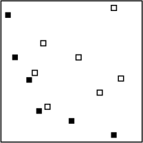
Figure 1: Illustration of the efficient set in two-dimensions. Filled squares are on the efficient set and unfilled squares are not. Only four of the filled squares are on the convex hull.

In the special case $k=d$, the expected size of the efficient set, $E_{d}(N)\equiv A_{d,d}(N)$, obeys the recursion

$$E_{d}(N)=E_{d}(N-1)+\frac{1}{N}\,E_{d-1}(N).$$ (17)

The point with the largest $x_{d}$ coordinate certainly does not dominate any other point. Furthermore, this point is on the efficient set if and only if the rest of its $d-1$ coordinates are not dominated by any other point. This event occurs with probability $\frac{1}{N}E_{d-1}(N)$ and hence, the second term in the recursion. We note that the recursion (17) can also be obtained by performing the integration over $x_{d}$ in $E_{d}(N)=N\int d{\bf x}\,[1-x_{1}x_{2}\cdots x_{d}]^{N-1}$. This integration is analytically feasible only if $k=1$ or $k=d$.

The recursion relation (17) is subject to the boundary condition $E_{1}(N)=1$. In two dimensions,

$$E_{2}(N)=1+\frac{1}{2}+\frac{1}{3}+\cdots+\frac{1}{N},$$ (18)

or alternatively, $E_{2}(N)=H(N)$, where $H(N)=\sum_{n=1}^{N}\frac{1}{n}$ is the harmonic number. The average size of the efficient set grows logarithmically, $E_{2}(N)=\ln N+\gamma+\cdots$ where $\gamma=0.57721$ is Euler’s constant. In three dimensions, we have $E_{3}(N)=\sum_{n=1}^{N}\frac{1}{n}H(n)$, and asymptotically, $E_{3}(N)\simeq\frac{1}{2}(\ln N)^{2}$. The large-$N$ behavior is obtained in general by converting the difference equation (17) into a differential equation $dE_{d}/dN=E_{d-1}/N$. The expected size of the efficient set grows logarithmically,

$$E_{d}(N)\simeq\frac{1}{(d-1)!}(\ln N)^{d-1}.$$ (19)

This logarithmic growth reflects that the integral of the scaling function, $\int d{\bf z}\,\Phi_{d,d}({\bf z})$, is divergent at the upper limit. A straightforward generalization of the calculation above shows that the distribution of the extremal coordinates has a logarithmic correction,

$$Q_{j}(y_{j})\sim(\ln N)^{d+1-j}(y_{j})^{-1}|\ln y_{j}|^{j-1},$$ (20)

for $1\leq j\leq d-1$. We can verify that the average number of points is consistent with the exact behavior $\int_{N^{-1/d}}dy\,Q_{j}(y_{j})\sim(\ln N)^{d-1}$ as in (19). The crossover moment vanishes and the moments decay logarithmically,

$$\langle y_{j}^{m}\rangle\sim(\ln N)^{-j},$$ (21)

where $m>0$ and $1\leq j\leq d-1$.

Two-dimensions. In two-dimensions, the full probability distribution function $p_{n}(N)$ that the efficient set includes $n$ points, where $1\leq n\leq N$, satisfies the recursion extremes

$$p_{n}(N)=\left(1-N^{-1}\right)p_{n}(N-1)+N^{-1}p_{n-1}(N-1)$$ (22)

and is subject to the boundary condition $P_{n}(0)=\delta_{n,0}$. On the square, there are two coordinates: $x_{1}$ and $x_{2}$. Following the reasoning behind (17), the point with the largest $x_{2}$ coordinate is on the efficient set if and only if its $x_{1}$ coordinate is minimal, an event that occurs with probability $N^{-1}$.

Recursion equations for the average $E(N)=\langle n\rangle$ and the variance $V(N)=\langle n^{2}\rangle-\langle n\rangle^{2}$ with $\langle f(n)\rangle\equiv\sum_{n=1}^{N}f(n)P_{n}$ are obtained by summing (22). The average satisfies $E(N)=E(N-1)+N^{-1}$ in accord with (17) and the variance satisfies $V(N)=V(N-1)+N^{-1}-N^{-2}$. Thus, the variance equals the difference between the first and the second harmonic numbers

$$V(N)=H(N)-H^{(2)}(N)$$ (23)

where $H^{(2)}(N)=\sum_{n=1}^{N}n^{-2}$. The variance and the average have identical leading asymptotic behaviors, $V(N)=\ln N+(\gamma-\frac{1}{6}\pi^{2})+\cdots$.

With the transformation $p_{n}(N)=\frac{1}{N!}\tilde{p}_{n}(N)$, the auxiliary function $\tilde{p}_{n}(N)$ satisfies the recursion

$$\tilde{p}_{n}(N)=(N-1)\tilde{p}_{n}(N-1)+\tilde{p}_{n}(N-1)$$ (24)

with $\tilde{p}_{n}(0)=\delta_{n,0}$. This recursion defines the Stirling numbers ${N\brack n}$ gkp so $\tilde{p}_{n}(N)={N\brack n}$. Therefore, the full probability distribution is expressed in closed form,

$$p_{n}(N)=\frac{1}{N!}\,{N\brack n}$$ (25)

for $0\leq n\leq N$.

The general asymptotic behavior, derived in bk ,

$$p_{n}(N)\simeq\frac{1}{N}\frac{1}{\Gamma(n/\ln N)}\,\frac{(\ln N)^{n}}{n!}$$ (26)

applies in the limit $n\to\infty$ $N\to\infty$ with the ratio $n/\ln N$ finite. For small $n\ll\ln N$, the distribution is Poissonian, $P_{n}(N)=N^{-1}(\ln N)^{n-1}/(n-1)!$ and for large $n$, the distribution approaches a Gaussian centered at the average $E(N)\simeq\ln N$ with the variance $V(N)\simeq\ln N$,

$$p_{n}(N)\to\frac{1}{\sqrt{2\pi\ln N}}\,\exp\left[-\frac{(n-\ln N)^{2}}{2\ln N}\right].$$ (27)

We note that the convex hull, a subset of the efficient set (see figure 1), is characterized by similar statistical properties including a limiting Gaussian distribution and logarithmic growths, albeit with different prefactors, of the average and the variance ars ; be ; vv .

Multi-Objective Shortest Path. The multi-objective shortest path on a graph is defined as follows. Consider a graph, possibly with multiple edges connecting pairs of nodes, with $d$ different costs on each edge. Fix the source and the destination nodes, and then consider all possible paths from source to destination, assigning a vector of $d$ total costs to each path. The multi-objective shortest path problem requires identification of the efficient set of paths. Generally, finding the efficient set is an NP-hard problem, although efficient approximation schemes exist approx1 ; approx2 . The computation time of the approximation scheme depends crucially on the size of the efficient set.

Suppose the weights are assigned independently at random to the edges. We can consider two limiting topologies. First, for a graph of two nodes connected by $N$ edges, the efficient set grows only polylogarithmically in the number of edges following the calculation above. Second, for a one-dimensional chain of nodes where each pair of neighboring nodes is connected by a pair of edges, the weights of the paths become correlated approx1 . We have conducted numerical studies, and found that the size of the efficient set is highly sensitive to the distribution of weights on the edges. Assuming each edge has two weights, $(w_{1},w_{2})$, both chosen from some continuous distribution, the convex hull grows linearly in the length of the chain. Interestingly, we observed various behaviors for the size of the efficient set, ranging from linear in the length of the chain, to power law behavior with various exponents greater than unity, up to stretched exponential behavior.

Finally, consider an Erdös-Renyi random graph of $M$ nodes bb ; jlr . Two randomly chosen nodes will typically have a shortest path distance between them of order $\log M$ using a metric which simply counts the number of edges traversed. While it is possible for a path on the efficient set to be longer than this, because the weights are positive, we expect that paths on the efficient set will be at most of order $\sqrt{\log M}$ longer. The total number of paths of at most that length grows exponentially in $\sqrt{\log M}$, and such paths will tend to overlap only near the source and destination nodes. Thus, to a good approximation we expect that the weights of the paths will be uncorrelated, enabling us to use the results above. Then, the number of paths on the efficient set will only be of order $(\log M)^{d/2}$. In general, then, when the paths have little overlap as here, the number of paths on the efficient set is much smaller than in cases like one-dimension where the paths greatly overlap.

Conclusions. We studied statistical properties of partial minima in a set of uncorrelated points in general dimensions. These partial minima are defined by a parameter $k$: a point is a partial minimum if it dominates all other points on at least $d-k$ coordinates. As this condition becomes more stringent, partial minima improve in quality but are less probable. Remarkably, there is a series of distinct power-law distributions that characterize the largest coordinates with a consequent multiscaling distribution of the moments, while the rest of the coordinates obey ordinary scaling. In the extreme case $k=d$, the number of partial minima grows logarithmically with the total number of points.

Our results hold as long as the set of points are not correlated, that is, as long as they are drawn from independent distributions. These distributions need not be identical. If the $i$th coordinate is drawn from the distribution $f_{i}(x_{i})$, the transformations $x_{i}\to\int_{0}^{x_{i}}dy_{i}f_{i}(y_{i})$ and $dx_{i}\to f_{i}(x_{i})dx_{i}$, maps to a uniform distribution in the unit hypercube. Correlations present an interesting challenge and we anticipate serious modifications to the scaling laws above. For instance, it is simple to show that the size of the efficient set grows as a power of the number of points, $\sim N^{1/2}$, rather than a logarithm, when the points are uniformly distributed inside the unit circle. Incidentally, this growth is much faster than the $N^{1/3}$ for the corresponding number of points in the convex hull ars .

Another interesting issue is the crossover from the algebraic decay (2) to the logarithmic growth (19). The average number of partial minima decreases monotonically with $N$ when $k$ is small, but is a non-monotonic function of $N$ when $k$ is large. For example, when $d=4$ and $k=3$, the average $A_{d,k}$ peaks at $N=16$. It will be interesting to elucidate how the height and the location of this peak scales with $N$.

Acknowledgments. We thank Gunes Ercal-Ozkaya for suggesting random graphs and Paul Krapivsky for useful discussions on convex hulls. We acknowledge financial support from DOE grant DE-AC52-06NA25396.

References

- (1) R. E. Steuer, Multiple Criteria Optimization: Theory, Computations, and Application (Wiley, New York, 1986).
- (2) Y. Sawaragi, H. Nakayama, and T. Tanino, Theory of Multiobjective Optimization, (Academic Press, Orlando, 1985).
- (3) D. Fudenberg and J. Tirole, Game Theory, (MIT Press, Cambridge, 1983)
- (4) M. J. Osborne and A. Rubenstein, A Course in Game Theory, (MIT Press, Cambridge, 1994).
- (5) M. Mézard, G. Parisi, and M. Virasoro, Spin Glass Theory and Beyond (World Scientific, Singapore, 1987).
- (6) B. Derrida and J. L. Lebowitz, Phys. Rev. Lett. 80, 209 (1998).
- (7) E. Ben-Naim, P. L. Krapivsky, and S. N. Majumdar, Phys. Rev. E 64, 035101 (2001).
- (8) G. Korniss, Z. Toroczkai, M. A. Novotny, and P. A. Rikvold, Phys. Rev. Lett. 84, 1351 (2000).
- (9) P. L. Krapivsky and S. Redner, Phys. Rev. Lett. 89, 258703 (2002).
- (10) For small , these integrals can be calculated manually or through recursion formulas. For example, when .
- (11) E. J. Gumbel, Statistics of Extremes (Columbia University Press, New York, 1958).
- (12) J. Galambos, The Asymptotic Theory of Extreme Order Statistics (R.E. Krieger Publishing Co., Malabar, 1987).
- (13) R. E. Ellis, Entropy, Large Deviations, and Statistical Mechanics (Springer-Verlag, New York, 1985).
- (14) Formally, when then .
- (15) T. Ottmann, E. Soisalon-Soininen, and D. Wood, Info. Sci. 33, 157 (1984).
- (16) E. Fink and D. Wood, Jour. Geometry 62, 99 (1998).
- (17) Generally, .
- (18) R. L. Graham, D. E. Knuth, and O. Patashnik, Concrete Mathematics: A Foundation for Computer Science (Reading, Mass.: Addison-Wesley, 1989).
- (19) E. Ben-Naim and P. L. Krapivsky, J. Phys. A 37, 5949 (2004).
- (20) A. Rényi and R. Sulanke, Z. Wahrsch. Verw. Geb. 2, 75–84 (1963).
- (21) B. Efron, Biometrika, 52, 331 (1965).
- (22) V. Vu, Adv. Math. 207, 221–243 (2006).
- (23) A. Warburton, Oper. Res. 35, 70 (1987).
- (24) G. Tsaggouris and C. Zaroliagis, Lect. Notes in Comp. Sci. 4288, 389 (2006).
- (25) B. Bollobás, Random Graphs (Academic Press, London, 1985).
- (26) S. Janson, T. Łuczak, and A. Rucinski, Random Graphs (John Wiley & Sons, New York, 2000).