Point Sources from a Spitzer IRAC Survey of the Galactic Center

Abstract

We have obtained $Spitzer$/IRAC observations of the central 2.0^∘$\times$ 1.4^∘($\sim$ 280 $\times$ 200 pc) of the Galaxy at 3.6µm–8.0µm. A point source catalog of 1,065,565 objects is presented. The catalog includes magnitudes for the point sources at 3.6, 4.5, 5.8, and 8.0µm, as well as $JHK_{s}$ photometry from 2MASS. The point source catalog is confusion limited with average limits of 12.4, 12.1, 11.7, and 11.2 magnitudes for [3.6], [4.5], [5.8], and [8.0], respectively. We find that the confusion limits are spatially variable because of stellar surface density, background surface brightness level, and extinction variations across the survey region. The overall distribution of point source density with Galactic latitude and longitude is essentially constant, but structure does appear when sources of different magnitude ranges are selected. Bright stars show a steep decreasing gradient with Galactic latitude, and a slow decreasing gradient with Galactic longitude, with a peak at the position of the Galactic center. From IRAC color-magnitude and color-color diagrams, we conclude that most of the point sources in our catalog have IRAC magnitudes and colors characteristic of red giant and AGB stars.

1 Introduction

Our Galactic center (GC), at a distance of $\sim$ 8.0 kpc (Reid, 1993), is the closest galactic nucleus, observable at spatial resolutions unapproachable in other galaxies (1 pc$\approx$26″). The region has been intensely studied at wavelengths outside the optical and UV regime, because it is unobservable with optical telescopes due to obscuring dust in the Galactic plane. The typical extinction toward the inner 200 pc is 25-30 visual magnitudes (Schultheis et al., 1999; Dutra et al., 2003), and it is considerably higher towards molecular clouds located close to the GC.

The extent of the GC region is defined by a region of relatively high density molecular gas ($n_{H_{2}}$ $\sim$ $10^{4}$ cm^-3; Bally et al. 1987), covering the inner 200 pc (170′$\times$ 40′, centered on the GC), called the Central Molecular Zone (CMZ). The CMZ produces 5%-10% of the Galaxy’s infrared and Lyman continuum luminosity and contains 10% of its molecular gas (Bally et al., 1987; Morris and Serabyn, 1996). The CMZ contains extremely dense giant molecular clouds (Martin et al., 2004; Oka et al., 2005; Boldyrev and Yusef-Zadeh, 2006), which are also very turbulent. Strong tidal shearing forces arise within the CMZ from a gravitational potential well that increases as the galactocentric radius decreases (Güsten and Downes, 1980), culminating in the central black hole, Sgr A^∗ (e.g. Schödel et al., 2003; Ghez et al., 2005).

In the past, the study of the GC stellar population has been concentrated primarily on the spatial regions surrounding three clusters of stars. The Central Cluster contains the dense core of stars within a few parsecs of the GC. The cluster is composed of a mixture of red supergiant and giant stars (e.g. Lebofsky et al., 1982; Sellgren et al., 1987) and young massive stars which exhibit energetic winds as observed in their emission line spectra (e.g. Allen et al., 1990; Krabbe et al., 1991; Libonate et al., 1995; Blum et al., 1995; Tamblyn et al., 1996). These bright, hot emission line stars trace an epoch of star formation that occurred about $10^{7}$ yr ago, while the bright cool stars may be associated with either the most recent epoch of star formation or older ones (Haller, 1992; Krabbe et al., 1995). The separation of bright cool stars into M supergiants (tracers of recent star formation) and less massive giants (tracers of older star formation) has been used to study the star formation history within the central cluster (Lebofsky et al., 1982; Sellgren et al., 1987; Blum et al., 1996, 2003). The Quintuplet and Arches Clusters are located at about 30 pc in projection from the GC. Both clusters contain hundreds of massive O-B stars, and have ages of 2–4 Myr (Figer et al., 1999) These clusters are thought to be the low-mass analog of the young “super star clusters” found in external galaxies (Allen et al., 1990; Nagata et al., 1996; Cotera et al., 1996; Figer et al., 1999).

One stellar population that has been studied across a broader area ($\sim$200 pc) centered on the GC is the OH/IR stars (Habing et al., 1983; Lindqvist et al., 1992; Sjouwerman et al., 1998, among others). OH/IR stars are oxygen rich Asymptotic Giant Branch (AGB) stars that are characterized by long period pulsations and high mass loss. Studies suggest that there are two distinct populations of OH/IR stars observed towards the GC, which are separated both spatially and kinematically (Lindqvist et al., 1992). The OH/IR stars that are more closely confined to the Galactic plane and that have a net prograde rotational velocity in the GC are also found to have higher OH maser expansion velocities than other OH/IR stars in the GC (Lindqvist et al., 1992). A higher expansion velocity requires either that the star is more luminous than the average (thus a more massive and younger star), or that it has a higher dust-to-gas ratio (and thus a higher metallicity).

Four other infrared studies have surveyed areas within 200 pc including the CMZ. The 2MASS all sky survey (Skrutskie et al., 2006) and the DENIS survey (Epchtein et al., 1997) were limited by their wavelength range between 1.2 and 2.2µm  which was inadequate to characterize the more obscured regions. The Midcourse Space Experiment (MSX) observed between 6 and 25µm and included the CMZ in its survey of the Galactic plane (Price et al., 2001). The angular resolution of MSX (18″ at 8.3µm), however, was only sufficient to identify the brightest isolated individual stars. Finally, portions of the CMZ were observed with ISOCAM as part of the ISOGAL survey, with $\sim$6″ angular resolution at 7µm and $\sim$13″ angular resolution at 15µm (Omont et al., 2003). The ISOGAL survey has been used to select young stellar object (YSO) candidates in the GC (Felli et al., 2002; Schuller et al., 2006) within the restricted area coverage of the survey.

We have obtained $Spitzer$/IRAC observations of the central 2.0^∘$\times$ 1.4^∘($\sim$ 280 $\times$ 200 pc, including the CMZ) of the Galaxy at 3.6µm–8µm in Cycle 1 (GO 3677, PI: Stolovy). These data represent the highest spatial resolution ($\sim$2″) and sensitivity uniform large-scale map made to date of the GC at mid-infrared wavelengths. The IRAC data display complex filamentary structures in the interstellar medium (S. Stolovy et al. 2007, in preparation) and allow us to detect optically obscured stellar sources. In this paper, we present details on the data reduction and point source extraction (Section 2). A catalog of the IRAC point sources band merged with 2MASS photometry is presented in Section 3. This catalog contains 1,065,565 point sources uniformly covering the CMZ. The point source magnitude distributions are discussed in Section 4 and the point source distributions with Galactic coordinates are examined in Section 5. A discussion of the nature of the point sources in the catalog is presented in Section 6. This is the first paper in an upcoming series on the $Spitzer$/IRAC observations of the Galactic center.

2 Observations and Data Processing

The InfraRed Array Camera (IRAC, Fazio et al., 2004) on board the Spitzer Space Telescope (Werner et al., 2004) was used to map the central regions of the Galaxy, with a spatial coverage of about 2.0^∘ in Galactic longitude by 1.4^∘ in Galactic latitude. Details of the observations and data processing are given in S. Stolovy et al. (2007, in preparation) but we provide a brief summary here.

Each IRAC detector has a 5.2′$\times$ 5.2′ field of view comprised of 256$\times$256 pixels and a mean pixel scale of 1.22″ per pixel. The four cameras have wavelengths of 3.6µm, 4.5µm, 5.8µm, and 8.0 µm  for Channels 1, 2, 3, and 4, respectively. Because all four cameras do not see the exact same region of sky simultaneously and because of orientation constraints, a larger region was mapped to cover fully the desired central 2.0^∘ $\times$ 1.4^∘  region. We used the shortest frame time (2 sec.) available for the full-array mode, corresponding to an on-source effective integration time of 1.2 seconds per pixel. We took five dithered exposures (or frames) on the sky for each pointing, giving a total average on-sky integration time of 6 seconds. This dithering strategy allows us to correct for bad pixels, scattered light, and latent images and provided improved sampling of the point spread function. Additional processing as described in S. Stolovy et al. (2007, in preparation) was performed on the Spitzer Science Center (SSC) pipeline version S13.2 Basic Calibrated Data (BCD) products to correct various artifacts (scattered light, latent images, column pulldown, and banding), producing much improved BCD frames and mosaics. One electronic artifact that was not corrected due to its non-linear nature was the ‘bandwidth effect’. This artifact causes extra ‘sources’ to appear 4 pixels away (and in some cases 8 pixels away) from very bright sources in Channels 3 and 4 along the readout direction (IRAC Data Handbook, Version 3.0, Section 4.3.3). Thus, a few of these artifacts remain in our final mosaics.

Additional observations were taken in IRAC’s sub-array mode for areas in the survey that were affected by saturation. These regions include the Central Cluster and the Quintuplet cluster, plus 12 individual pointings. In sub-array mode, a small section of the array is read out (32 $\times$ 32 pixels = 40″ $\times$ 40″), and we used the shortest exposure time available of 0.02 sec.

2.1 Mosaicking

We used the SSC Mosaicking and Point source Extraction (MOPEX) package, version 030106 (available from the SSC web page ) to create mosaics, extract point sources, and create source subtracted mosaics of the full-array data. MOPEX is composed of a series of PERL scripts. We used mosaic.pl to create mosaics, apex.pl to detect and measure fluxes of point sources, and apex_qa.pl to create source subtracted images. The script mosaic.pl performs interpolation and co-addition of FITS images, with the additional functionality of detection of outliers. The outliers are due to radiation hits, hot pixels, and bad pixels. There are three outlier detection algorithms implemented within mosaic.pl. The single frame outlier detection algorithm performs spatial filtering within an individual BCD frame, flagging outliers above a user defined flux threshold, and below a user defined size. The multiframe outlier and the dual outlier detection algorithms determine outlier pixels by stacking pixels taken in different exposures but at the same spatial location. The BCD frames are spatially matched by coincident point sources. The multiframe outlier computes the statistics of the stacked pixels and finds the outliers above a user defined $\sigma$ threshold. The dual outlier detection algorithm first detects all sources above a user defined $\sigma$ threshold and then compares the number of detections for each spatial location to discriminate the outliers from the real sources.

The optimization of the parameters of the outlier detection algorithms for our confusion-limited data was the most challenging part of the creation of the mosaics. The single frame outlier and the dual outlier algorithms flagged many real point sources as outliers, even using the most conservative set of input parameters, mainly due to crowding of point sources in our images. Therefore, we adopted only the multiframe outlier detection algorithm with a conservative threshold of 50$\sigma$, 50$\sigma$, 60$\sigma$, and 25$\sigma$, for Channels 1, 2, 3, and 4 respectively, which gave satisfactory results in terms of the number of pixels flagged as outliers per BCD frame per unit of exposure time and the lack of real point sources flagged as outliers. The expected number of radiation hits in one single IRAC frame is approximately 3 to 6 pixels per second in Channels 1 and 2, and approximately 4 to 8 pixels per second in Channels 3 and 4. Our observations comprise a total of 2,895 individual BCD frames per channel, with an integration time of 1.2 s per frame. This predicts a total number of radiation hits of about 10,000-21,000 pixels in Channels 1 and 2, and about 14,000–28,000 pixels in Channels 3 and 4. The total numbers of flagged outliers determined by MOPEX using the parameters described above were about 26,000, 26,000, 32,000, and 14,000 pixels in Channels 1, 2, 3, and 4, respectively, which are similar to expected values.

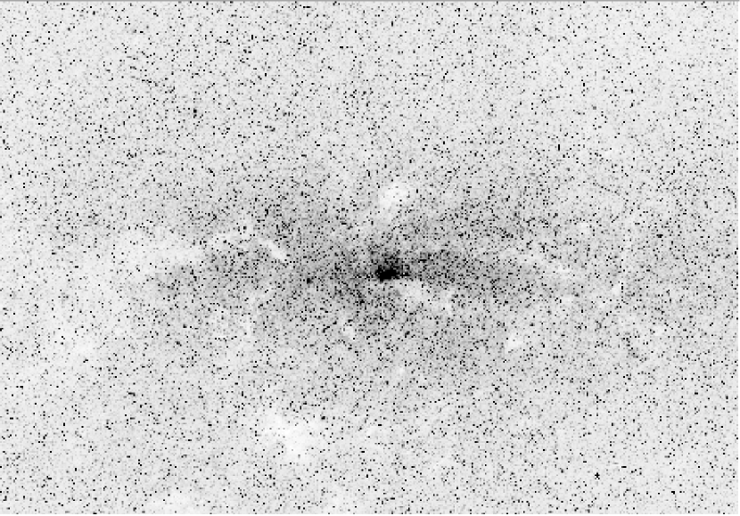
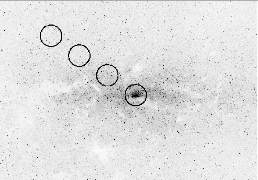
Figure 1: IRAC Channel 1 (3.6 µm) mosaic (top panel) and source subtracted mosaic (bottom panel) of the Galactic center, covering an area of 2.0^∘ $\times$ 1.4^∘, centered on $l$=0.0, $b$=0.0 (Galactic north is up, Galactic east is to the left). The mosaics are shown in reverse grayscale with the same scale. The circular areas shown in the bottom panel are centered on $l$=359.946, $b=-0.0378$; $l$=0.166, $b$=0.1162; $l$=0.386, $b$=0.2702; and $l$=0.606, $b$=0.4242. These circular areas are used in this paper to study the distribution of point sources in locations with different source densities.

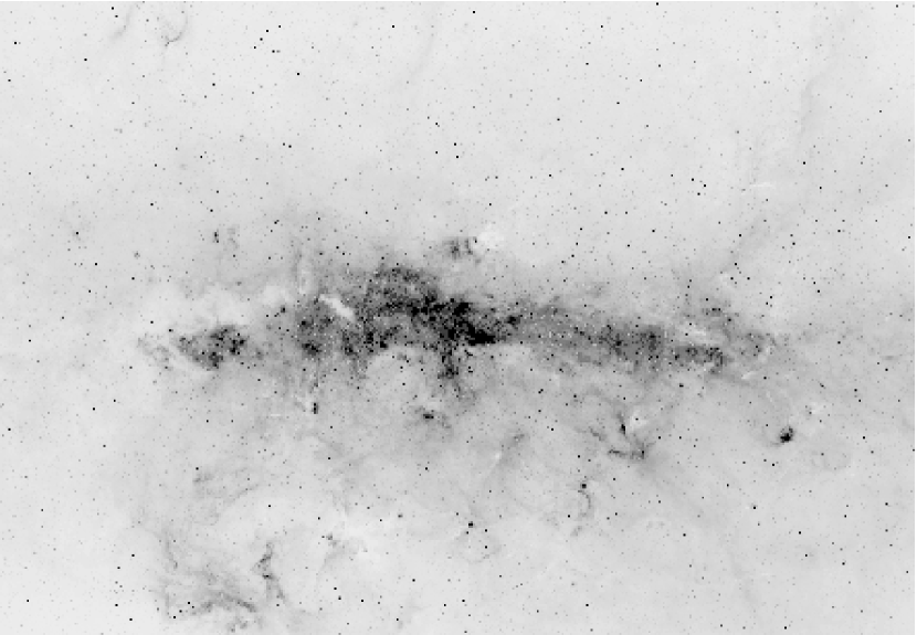
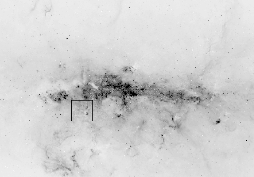
Figure 2: IRAC Channel 4 (8 µm) mosaic (top panel) and source subtracted mosaic (bottom panel) of the Galactic center, covering an area of 2.0^∘$\times$1.4^∘, centered on $l$=0.0, $b$=0.0 (Galactic north is up, Galactic east is to the left). The mosaics are shown in reverse grayscale with the same scale. The box plotted in the bottom panel shows the location of the blown up section detailed on Figure 3.

It is crucial to create a clean mosaic at each channel before attempting to extract the point sources. Our final mosaics represent a significant improvement over available SSC pipeline data products. The top panels of Figures 1 and 2 show the final full-array mosaics for Channels 1 and 4, covering a field of view of 2.0^∘$\times$ 1.4^∘, centered on $l$=0,0 and $b$=0.0 (see S. Stolovy et al. 2007, in preparation, for final mosaics including the sub-array observations).

2.2 Source extraction from full-array data

The source extraction was performed using the MOPEX script apex.pl, set up so it utilizes data products created with the MOPEX script mosaic.pl, in particular those concerning outlier detection. The script apex.pl performs the source detection in a background subtracted mosaic. It provides two measurements of the flux: one comes from a point response function (PRF) fitting and the other comes from an aperture measurement.

The PRF is the telescope point spread function convolved with the instrument response function. The algorithm that fits the PRF to the BCD sources allows a determination of the local background, which is advisable to use in crowded fields with variable background level such as those observed in the GC. Note that the flux uncertainty and the signal to noise ratio (SNR) as provided by apex.pl are the uncertainty and SNR of the PRF fitting algorithm. The PRFs used in the flux measurement were provided by the SSC.

The aperture flux measurement is performed on the mosaic image. The usual background estimates include performing the aperture measurement on a median filtered mosaic or using an annulus around the detected sources. Neither of these two methods for estimating the background are appropriate for our survey due to point source crowding and variable and high background levels. Instead, we used the local background determined by the PRF fitting to subtract the background contribution to the corresponding aperture flux. We measured the flux within a small aperture of 2 pixels radius (about 2.44″) to avoid confusion, then subtracted the background contribution, and finally applied the corresponding aperture correction. The value of the aperture corrections are 1.213, 1.234, 1.379, and 1.584 for Channels 1, 2, 3, and 4, respectively, as provided in the IRAC Data Handbook, Version 3.0. The script apex.pl does not provide a measure of the uncertainty of the aperture flux. We estimate the aperture flux uncertainty by performing an aperture measurement of the same size as the photometric aperture directly in the mosaic of the uncertainty images (data product of mosaic.pl).

The source extraction was performed in each of the 12 AORs separately because of the lack of enough computing memory to process the entire data set simultaneously. The resulting source lists for each AOR were combined to obtain a total source list for the whole survey. During this process we also rejected sources that were within a certain radius from a bright source ($\sigma$ threshold $>$ 30) and sources that were detected on top of extended emission in Channels 3 and 4. The radius of avoidance was 4.5″, 5.8″, 6.4″, and 8.3″ for Channels 1, 2, 3, and 4, respectively, which corresponds roughly to the radius of the second minimum of the diffraction pattern of the PRF. Note that rejecting faint sources within the radius of avoidance will also discard possible artifacts due to the 4-pixel bandwidth effect, present in Channels 3 and 4. The ‘bandwidth effect’ causes extra ‘sources’ to appear 4 pixels away (and in some cases 8 pixels away) from very bright sources in Channels 3 and 4 along the readout direction (IRAC Data Handbook, Version 3.0, Section 4.3.3). It is possible that some saturated sources were misidentified as many individual sources, each of them too faint to trigger the avoidance radius. To discriminate between a point source and an extended source, we use the fact that a point source should have the same aperture corrected flux independent of the size of the aperture used. We flagged a source as extended if the aperture corrected flux from a 3 pixel radius aperture differs by more than 15% from a 2 pixel radius aperture corrected flux. Sources flagged as extended are not included in the catalog.

We found that the PRF fluxes and aperture fluxes agreed to within 12% overall. We did, however, find that the PRF fluxes were systematically lower than the aperture fluxes by 13-12% for Channels 1 and 2, and higher by 7% for Channel 4. No significant difference was found for Channel 3. This difference is likely to arise from errors in PRF normalization. We measured the difference between the aperture fluxes and the PRF fluxes by first determining the IRAC colors of foreground sources with low amounts of reddening. Most of the foreground stars are expected to be red giant stars, whose IRAC colors should be near zero (M. Cohen, private communication; IRAC Handbook). Schultheis et al. (1999) and Dutra et al. (2003) have determined extinction maps at the Galactic center distance. The minimum extinction observed for a source located at the distance of the GC is $A_{K}$ = 1 magnitudes (Schultheis et al., 1999; Dutra et al., 2003). We therefore selected as foreground stars those sources with $A_{K}<$ 1 or $(J-K_{s})<$ 1.5. There are 6816 sources in our source list that have $(J-K)<$1.5, and their mean IRAC colors are listed in Table 1, for both PRF and aperture magnitudes. Aperture IRAC colors are closer to zero than PRF IRAC colors. The PRF method, however, is generally superior than aperture photometry in crowded fields, and also shows less scatter at fainter magnitudes. We adjusted the PRF fluxes for Channels 1, 2, and 4 such that the median ratio of the two extraction methods was 1. The multiplicative factors applied to the PRF fluxes were 1.13, 1.12, 1.00, and 0.93 for Channels 1, 2, 3, and 4 respectively. The IRAC colors of the final photometry are also listed in Table 1.

We produced point source-subtracted images, using the MOPEX script apex_qa.pl, to assess the effectiveness of the extraction and to compare the flux results obtained with the PRF fitting and aperture photometry. We found that the PRF fitting occasionally failed, producing a flux that was much too high. For the cases where the adjusted-PRF/aperture flux ratio exceeded 1.5, we adopted the aperture value of the flux and its corresponding uncertainty was derived as described above. The source-subtracted residual images show even fainter sources but we did not attempt to extract them. Additionally, the brighter sources close to saturation are in the nonlinear regime and therefore do not match the shape of the PRF. We did not attempt to subtract highly saturated sources.

The source subtracted mosaics for Channels 1 and 4 are shown in the bottom panels of Figures 1 and 2. The four circular areas shown in the bottom panel of Figure 1 will be used in Section 4 to study the distribution of point sources in different locations within our field of view. The circular areas have a radius of 5′ and they are centered on $l$=359.946, $b=-0.0378$; $l$=0.166, $b$=0.1162; $l$=0.386, $b$=0.2702; and $l$=0.606, $b$=0.4242.

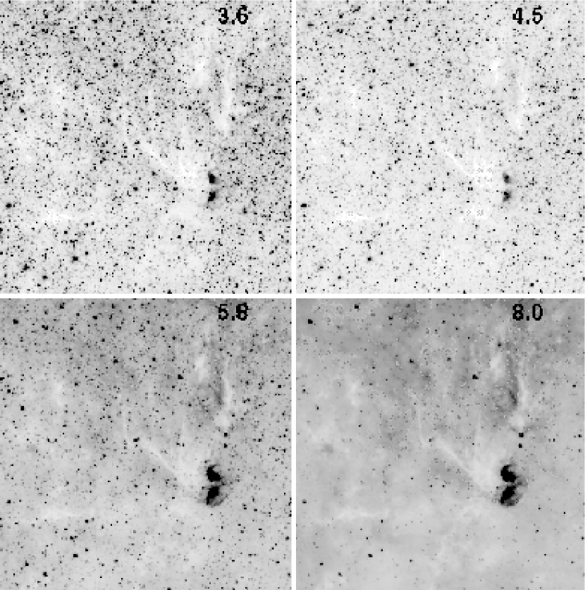
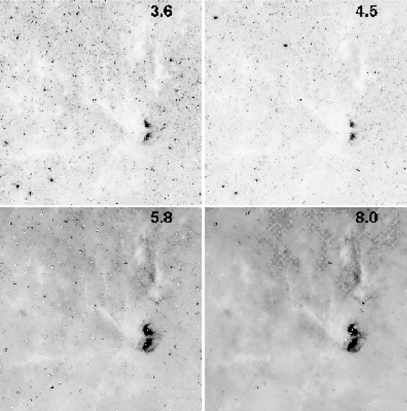
Figure 3: Detail of the IRAC mosaics and source subtracted mosaics showing 10′ $\times$ 10′ field of view, centered on ($l$=0.3523, $b$=$-0.17427$). The original mosaics are shown in the top set of four panels and the corresponding source subtracted images are shown in the bottom set. Each IRAC channel is labeled in the top right corner of the individual images. Note the differences in source densities and extended emission among the different IRAC channels. The residuals from the point sources are larger in Channel 1, and smaller in Channel 4, because the PRF is better sampled at longer wavelengths.

Figure 3 shows a 10′$\times$ 10′ field of view centered on ($l$=0.3523, $b$=$-0.17427$), marked as a box in the bottom panel of Figure 2. Figure 3 shows the differences in source densities and extended emission among the different IRAC channels. Residuals in Channel 4 are the smallest because the PRF is better sampled than in the other channels.

The total number of sources detected at a level of 3$\sigma$ or above in each channel was: 735,020, 700,923, 493,207, and 323,512 for Channels 1, 2, 3, and 4, respectively. All the sources detected and measured by MOPEX at the 3$\sigma$ level are listed in Table 2, 3, 4, and 5 (shown partially, available entirely in the electronic version). The columns of Table 2–5 are as follows: Source Identification, IRAC Channel, Position (Equatorial and Galactic), Flux in mJy, Flux uncertainty in mJy, Number of Observations (BCD frames used in the Flux measurement), Signal-to-noise ratio, and Flux Method as explained in the previous section.

The cumulative distribution of positional uncertainties is shown in Figure 4, for both right ascension (open symbols) and declination (filled symbols). The overall distributions of positional uncertainties are similar between right ascension and declination, for all four IRAC channels. We found that 90% of the sources in our survey have positional uncertainties less than 0.13″, 0.16″, 0.48″, and 1.18″ for Channels 1, 2, 3, and 4, respectively, corresponding to the typical positional uncertainties in our survey. Also, 99%, 96%, 59%, and 36% of the Channel 1, 2, 3, and 4 sources, respectively, have a positional uncertainty less than 0.2″. In the process of merging the IRAC point source lists with 2MASS (see details below), we found systematic offsets between IRAC positions in different channels and between the IRAC and 2MASS positions. These offsets are $\sim-$0.25″ in right ascension, and $\sim$0.15″ in declination, and have been applied to Ch. 1-4 such that the IRAC astrometry in all channels should now match the 2MASS astrometry in our final catalog.

Figure 5 shows the cumulative distribution of percentage flux uncertainty, derived as described above. The cumulative distribution of the percentage flux uncertainty for the four IRAC channels is shown in separate panels. The open symbols denote the cumulative distribution of percentage flux uncertainties for all the sources in each of the IRAC channels. We found that 90% of the sources in our survey have a percentage flux uncertainty less than 4.0%, 5.0%, 31% and 28% for Channels 1, 2, 3, and 4, respectively, corresponding to the typical percentage flux uncertainties in our survey. Also, 99%, 99%, 64%, 56% of the Channel 1, 2, 3, and 4 sources, respectively, have a percentage flux uncertainty less than 10%. The solid, dashed, and dotted lines in Figure 5 show the cumulative distribution of percentage flux uncertainties for sources of three different source brightness ranges, bright, medium, and faint, respectively, as defined in Section 4. The distribution of percentage flux uncertainties for Channels 3 and 4 is dominated by the distribution of percentage flux uncertainties for faint sources. Channels 3 and 4 mosaics show a wide range in background levels on top of which faint sources are measured. Variations in the local background may be the cause of the larger uncertainties in the flux measured in those channels.

2.3 Source extraction from sub-array data

In order to recover useful photometry from the small saturated regions in the full-array observations, we performed photometry on sub-array data, which consists of mosaics of the Central Cluster (SgrA) and the Quintuplet Cluster, plus 12 individual pointings. We used the interactive IDL program xstarfinder (Diolaiti et al., 2000), because the parameters used for the full-array data using MOPEX were not appropriate for the small sub-array observations. We also tested photometry using the IRAF source extraction program “daophot” but found that daophot gave less reliable results than xstarfinder.

The PRF was constructed from a composite of sub-array observations of well exposed, isolated single sources. These sources were chosen from the twelve individual pointing observations, excluding observations with higher than typical noise or with other stars within a $\sim$10″ radius of the main source. PRF’s were made using both xstarfinder and daophot and it was determined that the point source subtracted residual images were superior for the daophot PRFs; thus, the PRFs from daophot were used in the source extraction.

For each input mosaic, the surface brightness error per pixel was computed from each input mosaic directly. This error is photon-noise-dominated and well fit with a gaussian distribution. The flux errors for the extracted point sources are statistical only and do not reflect differences in the flux estimate that may arise from methodology, e.g., using a different set of extraction parameters such as the background smoothing box. We expect that the systematic errors may exceed the quoted random errors. The source extraction computes a correlation factor, which is a measure of the goodness of fit to the PRF, with 1.0 being a perfect fit. The correlation factor for all extracted sources was 0.75 at minimum, but most sources had a factor exceeding 0.9. A median smoothing size of 7 times the FWHM was used for the background determination.

Table 6 lists the sub-array photometric results including 13 sources in the dozen individual pointings or “sat” fields, 104 sources located in the Central Cluster or “sgra” field, and 90 sources located in the Quintuplet Cluster or “quint” field. The sub-array source table lists the brightness and its uncertainty in magnitudes for each IRAC Channel.

3 Catalog of Point Sources in the Galactic Center

We bandmerged our IRAC full-array source list for each channel with the sources in the 2MASS catalog (Skrutskie et al., 2006) located in the same field of view as our IRAC observations. The merging procedure was done as follows: We first matched and merged, via a positional association, Channel 1 and 2, then Channel 3, then Channel 4, and finally 2MASS. A match was defined as the closest counterpart within a 1″ radius. The position used for the final merged list was always that corresponding to the shortest IRAC wavelength at which a source is seen. The sub-array photometry was incorporated into the band merged list. The full-array photometry of each of the 13 sources in the “sat” fields was individually replaced by the sub-array photometry. All the sources with full-array photometry located within 40″ of the Central Cluster (RA=17 45 40.0, DEC=$-29$ 00 28) and within 42″ of the Quintuplet Cluster (RA=17 46 16.1, DEC=$-28$ 53 43) were discarded. The sub-array photometry of the “sgra” and “quint” fields were added to the band merged list.

The merged source list was further studied and additional flags regarding the detection reliability, position comments, and photometric quality were added. Magnitudes for each of the IRAC channels were computed using zero point fluxes of 280.9 Jy, 179.7 Jy, 115.0 Jy, and 64.13 Jy, for IRAC Channels 1, 2, 3, and 4 respectively, as provided by Reach et al. (2005).

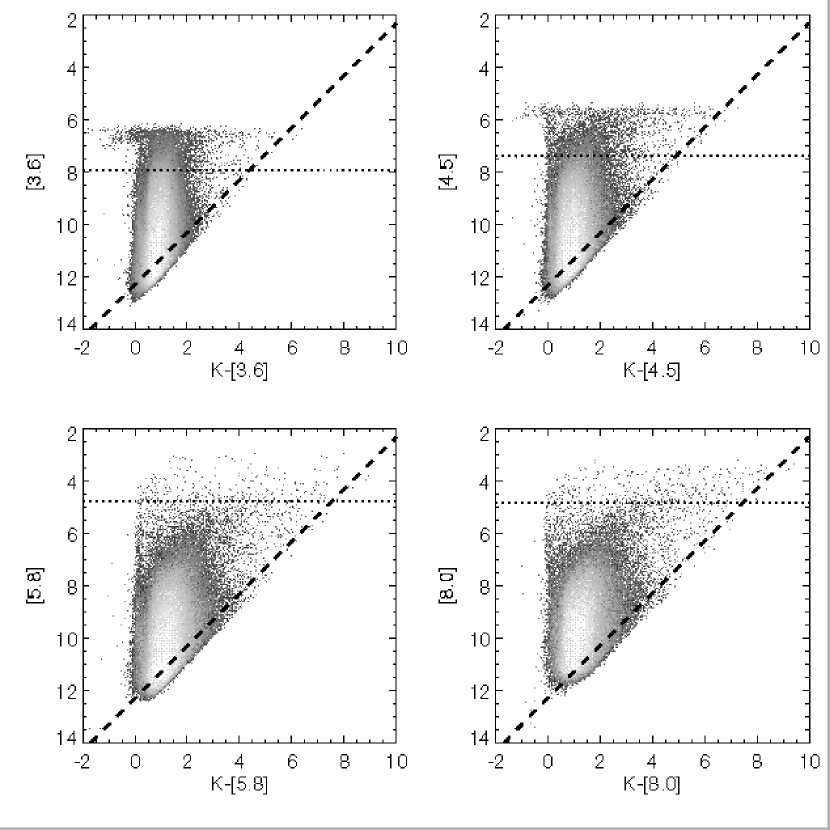
Figure 6: Color-magnitude diagrams (CMDs), or plots of the difference between $K_{s}$ and IRAC magnitude vs. IRAC magnitude. The CMD for the four IRAC magnitudes are shown in the corresponding panels. Only non-saturated high quality IRAC and $K_{s}$ magnitudes (IRAC magnitudes with SNR$>$10 and 2MASS photometric quality flag equal to ‘A’ (SNR$>$10)) are included in this figure. The gray scale shows the number density distribution of sources, with white being the highest density. The dotted line shows the magnitude corresponding to the saturation fluxes of 190 mJy, 200 mJy, 1400 mJy, and 740 mJy (7.92, 7.38, 4.79, and 4.84 magnitudes) for IRAC Channels 1, 2, 3, and 4 respectively, as provided by the $Spitzer$ Observer’s Manual (SOM). The dashed lines corresponds to the completeness limit of $K_{s}$=12.3 magnitudes of the 2MASS point source catalog within a 6^∘ radius of the Galactic center.

One of the qualities studied in the band merged source list was flux saturation for the full-array photometry. We needed to explore whether the saturation values for point sources provided by the IRAC documentation were appropriate for our survey. Figure 6 shows color magnitude diagrams (CMDs) using each IRAC magnitude and the $K_{s}$ magnitude from 2MASS (Skrutskie et al., 2006). Only non-saturated $K_{s}$ magnitudes with 2MASS photometric quality flags (ph_qual) equal to ‘A’ (SNR$>$10) are included in Figure 6. The gray scale shows the number density distribution of sources, with white being the highest density. Any anomalies in the bright regime of the CMDs are due to non-linear and saturation effects in the IRAC magnitudes. The horizontal dotted lines show the magnitudes corresponding to the saturation fluxes of 190 mJy, 200 mJy, 1400 mJy, and 740 mJy (7.92, 7.38, 4.79, and 4.84 magnitudes) for IRAC Channels 1, 2, 3, and 4 respectively, as provided by the $Spitzer$ Observer’s Manual, Version 7.1. The slanted dashed lines correspond to the completeness limit of $K_{s}$=12.3 for the 2MASS point source catalog within a 6^∘ radius of the Galactic center (see Sec IV.7, Cutri et al., 2003). Figure 6 also demonstrates that the saturation fluxes provided by the $Spitzer$ Observer’s Manual (Version 7.1) are indeed appropriately applied to our survey, as can be seen from the anvil-shaped tops of the CMDs for Channels 1 and 2. Note that the point source fluxes are superimposed on a high background, and the combination of both is likely to explain the saturation level appearing to be conservative when it really is appropriate. Saturated sources are retained in our point source catalog, as long as they are recognized as a point source by the apex.pl script. If the flux of a source is greater than the saturation flux provided by the $Spitzer$ Observer’s Manual, then all its measured quantities are kept in the catalog, but the flux flag of that source in that channel is set to ‘3’ in our final catalog.

The coverage of our survey has some incompleteness due to the fact that the four IRAC cameras do not see exactly the same region of the sky. The coverage for each source at each channel was determined by measuring the value of the pipeline coverage map at the position of each source. The coverage value is the same as the number of available BCD frames at the position of each source, and it is also listed in our final catalog for each channel. The location of each of the sources is flagged in our catalog by the Position flag. If a source is located in the area of incomplete coverage (coverage value is equal to zero in at least one channel), then the Position flag is set to ‘0’. Sub-array photometry has been incorporated into the catalog, in particular in the location near the Central Cluster and near the Quintuplet Cluster. If a source is located within 40″ of the Central Cluster (RA=17 45 40.0, DEC=$-29$ 00 28), the Position flag is set to ‘2’. If a source is located within 42″ of the Quintuplet Cluster (RA=17 46 16.1, DEC=$-28$ 53 43), the Position flag is set to ‘3’. The sources with Position flag set to ‘2’ and ‘3’ have photometry from the sub-array observations.

The reliability of the sources in our band merged list can be estimated by applying the “2+1” criterion as defined by the Galactic Legacy Infrared Mid-Plane Survey Extraordinaire (GLIMPSE) v1.5 Data Products Description (available from the GLIMPSE Documents web page ). The $M/N$ ratio is defined as the ratio between $M$ number of detections over $N$ number of possible observations (coverage value). The “2+1” criterion requires $M/N\geq 0.6$ in one IRAC band, $M/N\geq 0.4$ in an adjacent band. Sources that satisfy the GLIMPSE “2+1” criterion have the “2+1” flag set to ‘1’ in our final catalog.

Our final catalog of point sources in the Galactic center is listed in Table 7. The columns of our point source catalog are explained as follows:

Column 1, Source ID:

Designation of the detected source.

Column 2, R.A.:

Right Ascension in J2000.

Column 3, Dec.:

Declination in J2000.

Column 4, $l$:

Galactic Longitude.

Column 5, $b$:

Galactic Latitude.

Column 6, “2+1” Flag:

Set to ‘1’ when the source satisfies the GLIMPSE “2+1” criterion ($M/N\geq 0.6$ in one IRAC band, $M/N\geq 0.4$ in an adjacent band), set to ‘0’ otherwise.

Column 7, Pos. Flag.:

Set to ‘0’ when the source is located in areas of incomplete coverage, set to ‘2’ when the source is within 40″ of the Central Cluster, set to ‘3’ when the source is within 42″ of the Quintuplet Cluster, otherwise is set to ‘1’.

Column 8, 2MASS ID:

2MASS identification number from the 2MASS Catalog, set to ‘none’ when there is no 2MASS counterpart.

Column 9, $J$:

$J$ magnitude from the 2MASS Catalog, set to ‘$-9.999$’ when not detected.

Column 10, $J$ unc.:

Uncertainty of $J$ magnitude from the 2MASS Catalog, set to ‘$-9.999$’ when not measured.

Column 11, $H$:

$H$ magnitude from the 2MASS Catalog, set to ‘$-9.999$’ when not detected.

Column 12, $H$ unc.:

Uncertainty of $H$ magnitude from the 2MASS Catalog, set to ‘$-9.999$’ when not measured.

Column 13, $K_{s}$:

$K_{s}$ magnitude from the 2MASS Catalog, set to ‘$-9.999$’ when not detected.

Column 14, $K_{s}$ unc.:

Uncertainty of $K_{s}$ magnitude from the 2MASS Catalog, set to ‘$-9.999$’ when not measured.

Column 15, Qual. Flag:

Photometric quality flag (ph_qual) from the 2MASS Catalog. It is composed of three letters, one for each 2MASS filter ($JHK_{s}$). The letters can be: A (SNR $>$ 10), B (SNR $>$ 7), C (SNR $>$ 5), D (no SNR requirement), E (poor profile-fit photometry), F (detection without photometric uncertainty), U (detection with upper limit on magnitude), X (detection without brightness estimate). Set to ‘ZZZ’ when there is no 2MASS counterpart.

Column 16, ch1 ID:

Channel 1 identification number from point source list, also listed in Column 1 of Table 2, set to ‘none’ when there is no Channel 1 counterpart.

Column 17, [3.6]:

Channel 1 magnitude, computed using the Flux from Column 7 of Table 2, and the corresponding zero point flux, set to ‘$-9.999$’ when not detected in this IRAC channel.

Column 18, [3.6] unc.:

Uncertainty of Channel 1 magnitude, computed using the Flux and its uncertainty from Columns 7 and 8 of Table 2, and the corresponding zero point flux, set to ‘$-9.999$’ when not detected in this IRAC channel.

Column 19, [3.6] SNR:

Signal to Noise ratio of Channel 1 magnitude. set to ‘$-9.9$’ when not detected in this IRAC channel.

Column 20, ch1 Flag:

Channel 1 magnitude flag. Set to ‘1’ when flux and hence magnitude comes from PRF fitting algorithm, set to ‘2’ when flux and hence magnitude comes from aperture corrected measurement, set to ‘3’ when the full-array flux is greater than corresponding saturation limit, set to ‘4’ when the photometry comes from the sub-array observations, set to ‘0’ when there is no detection in this IRAC channel.

Column 21, ch1 Cov.:

Number of available BCD frames at the position of the source for the corresponding IRAC channel ($N$).

Column 22, ch1 $M/N$:

Ratio between $M$ number of detections over $N$ number of possible observations (ch1 Cov.).

Column 23, ch2 ID:

Same as Column 16, but for Channel 2.

Column 24, [4.5]:

Same as Column 17, but for Channel 2.

Column 25, [4.5] unc.:

Same as Column 18, but for Channel 2.

Column 26, [4.5] SNR:

Same as Column 19, but for Channel 2.

Column 27, ch2 Flag:

Same as Column 20, but for Channel 2.

Column 28, ch2 Cov.:

Same as Column 21, but for Channel 2.

Column 29, ch2 $M/N$:

Same as Column 22, but for Channel 2.

Column 30, ch3 ID:

Same as Column 16, but for Channel 3.

Column 31, [5.8]:

Same as Column 17, but for Channel 3.

Column 32, [5.8] unc.:

Same as Column 18, but for channel 3.

Column 33, [5.8] SNR:

Same as Column 19, but for Channel 3.

Column 34, ch3 Flag:

Same as Column 20, but for Channel 3.

Column 35, ch3 Cov.:

Same as Column 21, but for Channel 3.

Column 36, ch3 $M/N$:

Same as Column 22, but for Channel 3.

Column 37, ch4 ID:

Same as Column 16, but for Channel 4.

Column 38, [8.0]:

Same as Column 17, but for Channel 4.

Column 39, [8.0] unc.:

Same as Column 18, but for Channel 4.

Column 40, [8.0] SNR:

Same as Column 19, but for Channel 4

Column 41, ch4 Flag:

Same as Column 20, but for Channel 4.

Column 42, ch4 Cov.:

Same as Column 21, but for Channel 4.

Column 43, ch4 $M/N$:

Same as Column 22, but for Channel 4.

There are a total of 1,065,565 sources in our final catalog; 656,673 of those satisfy the GLIMPSE “2+1” criterion and have a SNR$>$ 10; they are considered to be highly reliable sources. We summarize other relevant statistics for our catalog in Table 8.

Two asteroids were found in the field of view at the time of our observations. Asteroid Alikoski appears in the final catalog as sources SSTGC 0629833 and SSTGC 0636843 (twice because it moved between Channel 3 and 4 coverage) and asteroid 459 Signe is in the final catalog as source SSTGC 0216539.

Areas close to the edges of our survey overlap with the GLIMPSE II (PI: Churchwell) observations. We have compared the photometry of our sources with SNR$>$10 to the photometry of the GLIMPSE II Highly Reliable Catalog. There are 184,392, 160,387, 132,077, and 72,065 sources positionally matched within 1″  between our catalog and GLIMPSE’s. The mean difference in magnitudes between our photometry and GLIMPSE is 0.11, 0.06, 0.00, and 0.03 for Channels 1, 2, 3, and 4. The standard deviations of the same differences are 0.15, 0.15, 0.17, and 0.18 magnitudes for Channels 1, 2, 3, and 4, respectively. The GLIMPSE photometry is expected to be have uncertainties less than 0.2 mags for most of its sources, according to the GLIMPSE Quality Assurance Document, v1.0. Thus, the observed differences are therefore less than the expected photometric uncertainties.

4 Magnitude Distributions

Figure 7 shows the magnitude distribution of point source detections for each of the channels in our survey. Only the sources located within the uniform coverage box ($-1.0\leq l\leq 1.0,-0.7\leq b\leq 0.7$) are included in the determination of the magnitude distributions. The open symbols show the magnitude distribution for all the sources and the filled symbols show the distribution for the sources which satisfy the “2+1” criterion and have a SNR greater than 10.

Figure 7 shows that the magnitude distributions have a similar shape in all the IRAC channels. There is a steep slope of increasing number of stars with increasing magnitude at the brightest magnitudes. This steep slope flattens around a bright turnover magnitude of 9.0, 8.6, 8.2, and 8.2 magnitudes for Channels 1, 2, 3 and 4, respectively. The number of stars increases more slowly with increasing magnitude at magnitudes fainter than the bright turnover. Finally, there is a faint cutoff followed by a steep slope of decreasing number of stars with increasing magnitude. The faint cutoff for all the sources (open symbols in Figure 7) is 12.4, 12.1, 11.7, and 11.2 for Channels 1, 2, 3, and 4, respectively. The faint cutoff for the sources which satisfy the “2+1” criterion and have SNR $>$ 10 (filled symbols in Figure 7) is 12.0, 11.8, 11.2, and 10.8 for Channels 1, 2, 3, and 4, respectively. Hereafter we define the bright magnitude range as those magnitudes brighter than the bright turnover magnitude, the medium magnitude range as those magnitudes between the bright turnover and the faint cutoff, and the faint magnitude range as those magnitudes fainter than the faint cutoff.

We plot a subset of magnitude distributions drawn from small regions within our GC mosaic, to understand features of the magnitude distribution. Only sources satisfying the “2+1” criterion and with SNR$>$10 are included in the determination of these magnitude distributions. Figure 8 shows the magnitude distributions of four circular areas located along a diagonal going away from the GC, but avoiding dark clouds, as plotted in the bottom panel of Figure 1. The solid, dotted, dashed and dashed-dotted lines show the magnitude distributions of these four locations in the order of increasing distance to the GC. There are about 2800, 2700, 2000, and 1200 sources in each 5′ radius circular area for Channels 1, 2, 3, and 4, respectively.

Figure 8 shows that, at this angular scale (10′), the magnitude distributions have the same shape as the magnitude distribution for the entire field of view (2.0^∘$\times$1.4^∘) as shown in Figure 7. The main difference among the magnitude distributions of the circular areas is that they seem to shift towards fainter magnitudes with increasing distance to the GC. As a consequence, the circular area located at the GC (solid line) has at least a factor of 3 more bright sources than the circular area located farthest from the GC (dashed-dotted line). For example at [3.6]=9.0, [4.5]=9.0, [5.8]=7.0, and [8.0]=7.5 magnitudes, the ratio of bright sources between the two areas is 3.0, 3.5, 5.0, and 5.5, respectively.

The faint cutoff of the magnitude distributions can be interpreted as due to confusion. Figure 8 shows that confusion is occurring at brighter magnitudes as one gets closer to the GC. The confusion limits suggested in Figure 8 for Channels 1 and 2 range from about 8.5 mag in the circular area located at the GC (solid line) to 13 mag in the circular area located the farthest away from the GC (dashed-dotted line). The same range of confusion limits for Channels 3 and 4 in Figure 8 is 8.0 (solid line) to 12.0 (dashed-dotted line).

The fact that we observe more bright sources with decreasing distance to the GC is consistent with previous population studies based on dereddened $K-$band luminosity functions. Blum et al. (1996) computed a dereddened $K-$band luminosity function within 1′ (2.3 pc) of the GC and compare it with a similar study at Baade’s Window in the bulge. Blum et al. (1996) found that both $K-$band luminosity functions had the same slope, but there was an overabundance of bright stars in the GC relative to Baade’s Window. Narayanan et al. (1996) constructed a dereddened $K-$band luminosity function for a region of 16′$\times$16′  (37$\times$37 pc) centered on the GC, but excluding the inner 2′ of the Galaxy. They found a luminosity function intermediate between that of Baade’s Window and the inner 2′ of the GC, having an excess of luminous stars over the bulge but not as many luminous stars as the inner 2′. Figer et al. (2004) obtained dereddened 2 µm luminosity functions, using high angular resolution observations. They computed synthetic luminosity functions using stellar evolution models and concluded that the observations were best fitted by models of continuous star formation.

All of the near infrared luminosity functions outside of the Central Cluster show the presence of a bright turnover. The luminosity function of the central 200 pc is known to have an excess of luminous stars relative to bulge fields such as Baade’s Window, and this excess of luminous stars increases closer to the GC (Catchpole et al., 1990; Blum et al., 1996; Narayanan et al., 1996; Philipp et al., 1999; Figer et al., 2004). The variation in the number of the brightest stars with distance to the GC over a large area may cause the presence of the bright turnover. This speculation is complicated by several effects. First, the bright turnover for Channels 1 and 2, at the areas close to the GC, occurs very close to the saturation limit (Ch. 1 and 2 magnitudes of 7.9 and 7.4, respectively). Second, the extinction and local background in the GC are highly spatially variable, even within a 10′ field of view. Finally, stellar crowding may artificially enhance the bright end of measured luminosity functions as pointed out by DePoy et al. (1993). Higher angular resolution surveys of the GC area may indeed improve our knowledge of the nature of the bright range sources seen in this survey.

The magnitude distribution shown in Figure 7 can be understood as the integral of individual magnitude distributions such as those plotted in Figure 8. The integral of the individual magnitude distributions is non-trivial to calculate due to the wide range in stellar density, extinction, background levels, and confusion within our field of view. Complete modeling of the observed magnitude distribution is beyond the scope of the present work and may be addressed in a future work.

5 Source distribution with Galactic Longitude and Latitude

The overall density of detected point sources with latitude and longitude is essentially constant, a consequence of being confusion limited. The relatively constant number of sources per circular area also indicates that our images are confusion limited. However, interesting structure along Galactic latitude and longitude does appear when we select sources within different magnitude ranges (defined above). The point source distributions along Galactic latitude and longitude in the different magnitude ranges are shown in Figures 9 and 10. The different panels show the distribution of the point sources for bright, medium, and faint, as indicated. Circles, triangles, squares, and pentagons correspond to the Galactic coordinate distributions of Channels 1, 2, 3, and 4, respectively.

The structure seen at the bright range is consistent with the fact that more bright sources are observed towards the GC (as discussed in Section 4). This agrees well with previous population studies that find an excess of luminous stars in the GC relative to bulge fields (Catchpole et al., 1990; Blum et al., 1996; Narayanan et al., 1996; Philipp et al., 1999; Figer et al., 2004).

The structure seen at the faint range is set by our ability to detect faint sources. The faint range contains sources below the lowest confusion limit for each channel, and therefore they follow the trend of the variation of the confusion with Galactic latitude and longitude.

The structure along Galactic latitude has a similar shape for all the IRAC channels, but some features are more prominent at longer wavelengths. The sources in the bright range show a steeply decreasing gradient with Galactic latitude, with a peak in the position of the Galactic center. The medium range sources show a slowly decreasing gradient with Galactic latitude. Those sources in the faint range show an increasing gradient with Galactic latitude, with the minimum at the position of the Galactic center.

Figure 10 illustrates that the structure along Galactic longitude also has the same shape for all the IRAC channels. The sources in the bright and medium brightness range show a slow decrease with Galactic longitude, with a peak at the position of the Galactic center. The sources in the faint range show an increase with Galactic longitude, with the minimum at the position of the Galactic center.

6 Color-Magnitude and Color-Color Diagrams

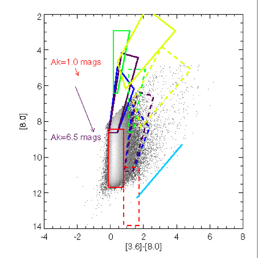
Figure 11: [8.0] vs. [3.6]-[8.0] color-magnitude diagram. The gray scale shows the number density distribution of sources, with white being the highest density. Only sources satisfying the “2+1” criterion and having SNR$>$10 are plotted. The arrows show the direction of the reddening vector, using the extinction law from Indebetouw et al. (2005), and the minimum ($A_{K}$=1.0) and maximum ($A_{K}$=6.5) amount of extinction measured towards the GC (Blum et al., 1996; Schultheis et al., 1999; Dutra et al., 2003). The locations of evolved stars are taken from the CMD of the $Spitzer$ SAGE LMC survey (Blum et al., 2006) and placed at the Galactic center distance: red giant stars ($red~{}boxes$), O-rich AGB stars ($blue~{}boxes$), C-rich AGB stars ($purple~{}boxes$), extreme AGB stars ($yellow~{}boxes$), and supergiant stars ($green~{}boxes$). The $solid~{}line~{}boxes$ show the location of objects assuming an extinction of $A_{K}$=1.0 magnitudes, and the $dashed~{}line~{}boxes$ show the same boxes assuming an extinction of $A_{K}$=6.5 magnitudes. The $cyan~{}line$ shows the position below which background galaxies should be located, assuming an extinction of $A_{K}$=1.0 magnitudes. The location of all the point sources with colors bluer than [3.6]-[8.0]=2.0 can be understood as evolved stars seen through varying amounts of extinction.

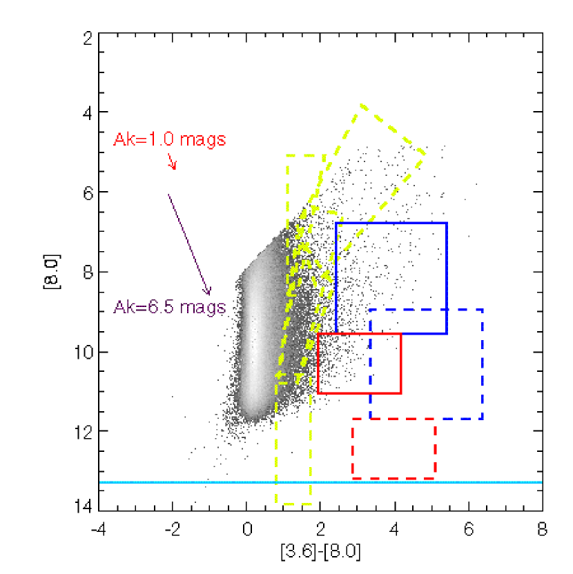
Figure 12: [8.0] vs. [3.6]-[8.0] color-magnitude diagram. The gray scale shows the number density distribution of sources, with white being the highest density. Only sources satisfying the “2+1” criterion and having SNR$>$10 are plotted. The arrows show the direction of the reddening vector, using the extinction law from Indebetouw et al. (2005), and the minimum ($A_{K}$=1.0) and maximum ($A_{K}$=6.5) amount of extinction measured towards the GC (Blum et al., 1996; Schultheis et al., 1999; Dutra et al., 2003). The $cyan~{}line$ shows the [8.0] magnitude of the brightest low-mass YSO observed in Taurus (Hartmannn et al., 2005) at Galactic center distance. The $red~{}boxes$ denote the location of 3.8 $M_{\odot}$ YSOs, and the $blue~{}boxes$ denote the location of 5.9 $M_{\odot}$ YSOs, as observed in the giant HII region RCW 49 by Whitney et al. (2004) and placed at the distance of the Galactic center. The dotted $yellow~{}boxes$ show the location of evolved stars, assuming an extinction of $A_{K}$=6.5 magnitudes, as shown in Figure 11, for reference.

Figures 11 and 12 show the [8.0] vs. [3.6]-[8.0] color-magnitude diagram (CMD) of all the sources satisfying the “2+1” criterion and having both [3.6] and [8.0] magnitudes with a SNR greater than 10. The gray scale shows the number density distribution of sources, with white being the highest density. The arrows show the direction of the reddening vector, using the extinction law from Indebetouw et al. (2005). The red arrow shows the amount of extinction for $A_{K}$=1.0, while the purple arrow shows the amount of extinction for $A_{K}$=6.5. According to the extinction maps of Schultheis et al. (1999) and Dutra et al. (2003) an extinction of $A_{K}$=1.0 is observed at the edges of our survey which we adopt as the minimum foreground extinction towards GC stars in our field of view. An extinction of $A_{K}$=6.5 was measured as the maximum observed extinction within 2′  of the Galaxy by the the near infrared photometric work of Blum et al. (1996). The highest density of points in the CMD shows a well defined sequence of constant [3.6]-[8.0] color, at a color of $\sim$0.2 mag. The distribution is skewed towards red colors, which is consistent with varying amounts of extinction.

To determine what types of objects are seen in our survey, we have overplotted the location of evolved stars in the CMD of Figure 11. The location of evolved stars is taken from the [8.0] vs. [3.6]-[8.0] CMD of stars in the $Spitzer$ SAGE survey of the Large Magellanic Cloud (Blum et al., 2006). They determined the location of the tip of the red giant branch, the O-rich and C-rich AGB stars, supergiant stars, and extreme AGB stars from the DENIS and 2MASS analysis of LMC stars by Cioni et al. (2006). We assume a distance modulus to the LMC of 18.48 magnitudes (Borissova et al., 2004), and a distance to the Galactic center of 8.0 kpc (Reid, 1993) to determine their location in our observed CMD. In Figure 11, the solid line boxes show the location of objects assuming an extinction of $A_{K}$=1.0 magnitudes, and the dashed line boxes show the same boxes assuming an extinction of $A_{K}$=6.5 magnitudes.

Blum et al. (2006) also noted the location of background galaxies in their CMD. The cyan line in Figure 11 shows the limit below which background galaxies should be observed, assuming an extinction of $A_{K}$=1.0 magnitudes. This line is at the edge of our observing limit, and it would be even lower if more extinction is added to it. We conclude that our survey is very unlikely to include background galaxies.

In Figure 11, different colored boxes illustrate the location of different types of stars, including red giants (red), O-rich stars (blue), C-rich stars (purple), extreme AGB stars (yellow), and supergiants (green). The bottom of the solid red giant box (at [8.0]=11.67 mag.) marks the [8.0] magnitude of a K0 III star located at the GC observed through $A_{K}$=1.0 magnitudes of extinction. There are 183,857 points sources plotted in figure 11. About 78% of the point sources shown (143,039 in total) lie within the limits of the red solid box denoting the location of the red giant stars with spectral types later than K0 III. The location of all the point sources with colors bluer than [3.6]-[8.0]=2.0 and with [8.0] magnitudes brighter than 8.0 can be understood as evolved stars seen through varying amounts of extinction with the range of values discussed above.

There are 917 sources in our catalog with [3.6]-[8.0] $\geq$ 2.0 and [8.0] $\geq$ 8.0. To explore the possibility of finding young stellar objects among these 917 red objects, we have overplotted the location of YSOs in the CMD of Figure 12. As in Figure 11, the solid line boxes show the location of objects assuming an extinction of $A_{K}$=1.0 magnitudes, and the dashed line boxes show the same boxes assuming an extinction of $A_{K}$=6.5 magnitudes. The cyan line shows the [8.0] magnitude of the brightest low-mass YSO observed in Taurus (Hartmannn et al., 2005), assuming a distance to Taurus of 140 pc. This line demonstrate that low-mass YSOs cannot be detected in our survey. Whitney et al. (2004) studied the giant HII region RCW 49, as part of the GLIMPSE legacy program. They determined the location of 2.5, 3.8, and 5.9 $M_{\odot}$ YSOs, using the radiative transfer models from Whitney et al. (2003). We assume a distance of 4.2 kpc to RCW 49 (Churchwell et al., 2004) and a Galactic center distance of 8 kpc (Reid, 1993) to determine their location in our observed CMD. The red boxes denote the location of the 3.8 $M_{\odot}$ YSOs, and the blue boxes denote the location of 5.9 $M_{\odot}$ YSOs. The dotted yellow boxes show the location of evolved stars, as reference, assuming an extinction of $A_{K}$=6.5 magnitudes, as shown in Figure 11.

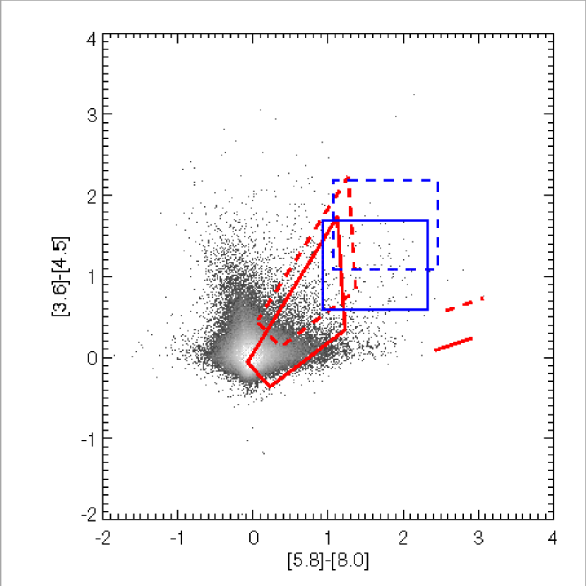
Figure 13: [3.6]-[4.5] vs. [5.8]-[8.0] color-color diagram. The gray scale shows the number density distribution of sources, with white being the highest. Only sources satisfying the “2+1” criterion and having SNR$>$10 are plotted. The $solid~{}line~{}boxes$ show the location of objects assuming an extinction of $A_{K}$=1.0 magnitudes, and the $dashed~{}line~{}boxes$ show the same boxes assuming an extinction of $A_{K}$=6.5 magnitudes. The $red~{}boxes$ show the average location of AGB star colors from Marengo et al. (2006). Marengo et al. (2006) also determine the location of an AGB star with a thick envelope (V354 Lac), which is shown with the $red~{}lines$. The $blue~{}boxes$ show the location of 3.8 $M_{\odot}$ and 5.9 $M_{\odot}$ YSOs (Whitney et al., 2004).

Figure 13 shows the [3.6]-[4.5] vs. [5.8]-[8.0] color-color diagram. The gray scale shows the number density distribution of sources, with white being the highest density. In Figure 13, the solid line boxes show the location of objects assuming an extinction of $A_{K}$=1.0 magnitudes, and the dashed line boxes show the same boxes assuming an extinction of $A_{K}$=6.5 magnitudes. Marengo et al. (2006) derived colors of AGB stars by convolving observed ISO spectra with IRAC bandpasses. The location of these derived IRAC colors are coincident with the models of Groenewegen (2006) computed using stellar atmosphere models with dust envelopes of different composition. The red boxes show the location of AGB star colors from Marengo et al. (2006). Marengo et al. (2006) also show that an AGB star with a thick envelope (V354 Lac) may have a unreddened [5.8]-[8.0] color between 2.4 and 2.9, and a unreddened [3.6]-[4.5] color between 0.05 and 0.15. The red line shows the location of V354 Lac with the corresponding amounts of extinction. The blue boxes show the location of 3.8 $M_{\odot}$ and 5.9 $M_{\odot}$ YSOs (Whitney et al., 2004). If we consider the typical uncertainties discussed in Section 2.2, the typical uncertainty in the [3.6]-[4.5] color is 0.06 magnitudes and the typical uncertainty in the [5.8]-[8.0] color is 0.42 magnitudes. There are 176,724 points sources plotted in Figure 13. About 38% of the point sources shown (66,988 in total) have zero IRAC colors within the typical uncertainties. These point sources have been exposed to little reddening, and hence they may be foreground objects or objects away from the Galactic plane.

As the GC is a known region of recent star formation, the possibility of observing a YSO population is an exciting prospect. We are likely to be sensitive only to the most massive YSOs (if present), at the distance of the GC, due to confusion. Our survey, however, contains sources observed at different distances and over varying amounts of extinction. We must carefully examine any candidate YSO population that we identify based on IRAC colors, to distinguish foreground YSOs (in the star forming arms along the line of sight, for instance) with a range of masses from massive YSOs at the GC. In addition, thick envelope AGB stars and YSOs have similar IRAC colors, and distinguishing one from the other will require additional diagnostics. Future work will include incorporating photometry at longer infrared wavelengths (e.g. ISOGAL, MSX and eventually MIPS 24 $\mu$m) and spectroscopy in order to best determine the nature of this population of objects with red IRAC colors.

7 Conclusions

Our conclusions can be summarized as follows:

• A point source catalog of 1,065,565 objects is presented. The catalog includes positions, $J$, $H$, $K_{s}$, [3.6], [4.5], [5.8], and [8.0] magnitudes, and a series of flags that assess the quality of the measurements.

• The point source catalog is confusion limited. The confusion limits vary by 2 to 3 magnitudes within the field of view. Nevertheless, the average confusion limits are 12.4, 12.1, 11.7, and 11.2 magnitudes for Channels 1, 2, 3, and 4, respectively.

• The overall distribution of point sources with Galactic latitude and longitude is essentially constant (a consequence of being confusion limited), but structure does appear when sources of different magnitude ranges are selected. Bright stars show a slow decrease in number density with Galactic longitude, and a steeper decrease with Galactic latitude, with a peak at the position of the Galactic center.

• Most of the point sources in our catalog have IRAC magnitudes and colors characteristic of red giant stars and AGB stars. There are several hundreds of extremely red objects, however, some of which may be massive YSOs. Follow up observations are needed to determine the nature of the extremely red objects.

Table 1: Mean IRAC colors of foreground sources.

Color	Mean	Std. Dev.	Mean	Std. Dev.	Mean	Std. Dev.
	PRF	PRF	Aperture	Aperture	Final	Final
[3.6]-[4.5]	0.02	0.15	0.02	0.13	0.01	0.15
[3.6]-[5.8]	0.23	0.25	0.08	0.26	0.11	0.25
[3.6]-[8.0]	0.37	0.42	0.10	0.45	0.16	0.42
[4.5]-[5.8]	0.22	0.18	0.06	0.19	0.10	0.18
[4.5]-[8.0]	0.35	0.38	0.08	0.41	0.15	0.38
[5.8]-[8.0]	0.13	0.34	0.02	0.36	0.05	0.34

Table 2: Galactic Center IRAC 1 Source Lists

Source ID	Channel	R.A.	Dec.	$l$	$b$	Flux	Flux Unc.	$N_{obs}$	S/N	Method
		(J2000)	(J2000)			(mJy)	(mJy)
GC-IRAC1-000001	1	17 40 11.07	-29 20 57.3	359.02435920	0.79220897	13.590	0.372	2	815.0	APC
GC-IRAC1-000002	1	17 40 11.15	-29 20 52.3	359.02569293	0.79268906	8.159	0.135	2	321.7	APC
GC-IRAC1-000003	1	17 40 11.19	-29 21 04.8	359.02283701	0.79073782	5.534	0.342	2	11.4	PRF
GC-IRAC1-000004	1	17 40 11.20	-29 21 14.0	359.02068282	0.78935613	2.645	0.116	2	5.7	PRF
GC-IRAC1-000005	1	17 40 11.70	-29 21 15.5	359.02129310	0.78760658	7.707	0.166	2	31.6	PRF
GC-IRAC1-000006	1	17 40 11.88	-29 21 04.3	359.02428009	0.78869809	2.875	0.103	2	16.5	PRF
GC-IRAC1-000007	1	17 40 11.89	-29 20 57.9	359.02581916	0.78959725	2.958	0.109	2	17.0	PRF
GC-IRAC1-000008	1	17 40 11.97	-29 16 23.4	359.09058043	0.82984460	1.704	0.081	2	12.9	PRF
GC-IRAC1-000009	1	17 40 12.26	-29 21 03.8	359.02512173	0.78758333	1.661	0.082	2	12.0	PRF
GC-IRAC1-000010	1	17 40 12.30	-29 16 14.5	359.09331294	0.83014414	13.470	0.227	2	86.2	PRF

Note. — Table 2 is published in its entirety in the electronic edition of the Astrophysical Journal. A portion is shown here for guidance regarding its form and content.

Table 3: Galactic Center IRAC 2 Source Lists

Source ID	Channel	R.A.	Dec.	$l$	$b$	Flux	Flux Unc.	$N_{obs}$	S/N	Method
		(J2000)	(J2000)			(mJy)	(mJy)
GC-IRAC2-000001	2	17 40 11.03	-29 28 01.2	358.92449479	0.72982023	12.768	0.554	2	124.3	PRF
GC-IRAC2-000002	2	17 40 11.48	-29 27 52.0	358.92753029	0.72979809	1.755	0.074	2	19.5	PRF
GC-IRAC2-000003	2	17 40 11.48	-29 28 02.5	358.92505842	0.72822659	2.197	0.086	2	21.4	PRF
GC-IRAC2-000004	2	17 40 11.81	-29 27 56.4	358.92712847	0.72814594	1.282	0.070	2	12.5	PRF
GC-IRAC2-000005	2	17 40 12.19	-29 23 09.4	358.99542952	0.76930396	20.899	0.290	2	93.5	PRF
GC-IRAC2-000006	2	17 40 12.21	-29 27 46.2	358.93030479	0.72838905	8.130	0.155	2	68.4	PRF
GC-IRAC2-000007	2	17 40 12.33	-29 22 59.1	358.99812850	0.77039026	1.567	0.077	2	10.0	PRF
GC-IRAC2-000008	2	17 40 12.58	-29 27 53.1	358.92940792	0.72623917	69.317	0.679	2	411.6	PRF
GC-IRAC2-000009	2	17 40 12.67	-29 23 06.4	358.99705877	0.76823969	41.474	0.482	2	236.6	PRF
GC-IRAC2-000010	2	17 40 12.78	-29 27 48.3	358.93092495	0.72633266	2.025	0.092	2	10.2	PRF

Note. — Table 3 is published in its entirety in the electronic edition of the Astrophysical Journal. A portion is shown here for guidance regarding its form and content.

Table 4: Galactic Center IRAC 3 Source Lists

Source ID	Channel	R.A.	Dec.	$l$	$b$	Flux	Flux Unc.	$N_{obs}$	S/N	Method
		(J2000)	(J2000)			(mJy)	(mJy)
GC-IRAC3-000001	3	17 40 11.66	-29 21 22.8	359.01949975	0.78664857	36.690	0.678	2	96.3	PRF
GC-IRAC3-000002	3	17 40 11.72	-29 21 15.4	359.02136276	0.78755549	3.452	0.254	2	15.3	PRF
GC-IRAC3-000003	3	17 40 12.31	-29 16 14.5	359.09332451	0.83010156	6.246	0.309	2	36.0	PRF
GC-IRAC3-000004	3	17 40 12.56	-29 21 15.5	359.02295870	0.78495848	8.214	0.324	2	38.2	PRF
GC-IRAC3-000005	3	17 40 12.67	-29 21 19.8	359.02215756	0.78396611	1.979	0.230	2	8.3	PRF
GC-IRAC3-000006	3	17 40 13.09	-29 16 34.1	359.09022025	0.82480989	2.374	0.229	2	12.2	PRF
GC-IRAC3-000007	3	17 40 13.17	-29 16 23.8	359.09280942	0.82608296	9.377	0.337	2	47.5	PRF
GC-IRAC3-000008	3	17 40 13.24	-29 16 40.2	359.08907321	0.82344698	29.050	1.770	2	149.5	PRF
GC-IRAC3-000009	3	17 40 13.30	-29 21 25.5	359.02202594	0.78121008	14.530	0.401	2	61.4	PRF
GC-IRAC3-000010	3	17 40 13.45	-29 25 34.0	358.96380980	0.74408637	41.970	2.710	2	105.3	PRF

Note. — Table 4 is published in its entirety in the electronic edition of the Astrophysical Journal. A portion is shown here for guidance regarding its form and content.

Table 5: Galactic Center IRAC 4 Source Lists

Source ID	Channel	R.A.	Dec.	$l$	$b$	Flux	Flux Unc.	$N_{obs}$	S/N	Method
		(J2000)	(J2000)			(mJy)	(mJy)
GC-IRAC4-000001	4	17 40 12.18	-29 32 20.1	358.86576803	0.68811768	3.358	0.261	2	49000.0	APC
GC-IRAC4-000002	4	17 40 12.23	-29 27 46.2	358.93034169	0.72836161	2.477	0.563	1	10.2	PRF
GC-IRAC4-000003	4	17 40 12.26	-29 23 20.6	358.99291905	0.76741035	4.660	0.489	2	20.0	PRF
GC-IRAC4-000004	4	17 40 12.58	-29 23 17.3	358.99431916	0.76693178	7.815	0.424	2	33.6	PRF
GC-IRAC4-000005	4	17 40 12.59	-29 27 53.1	358.92940149	0.72622137	24.106	0.649	2	77.2	PRF
GC-IRAC4-000006	4	17 40 12.68	-29 23 06.4	358.99707024	0.76821160	17.530	0.551	2	76.8	PRF
GC-IRAC4-000007	4	17 40 12.98	-29 23 16.1	358.99537641	0.76586405	1.402	0.336	2	5.1	PRF
GC-IRAC4-000008	4	17 40 12.99	-29 32 43.3	358.86187264	0.68219639	33.694	5.370	2	70.9	PRF
GC-IRAC4-000009	4	17 40 13.14	-29 23 19.0	358.99500161	0.76494954	2.809	0.378	2	13.2	PRF
GC-IRAC4-000010	4	17 40 13.28	-29 27 58.8	358.92940310	0.72326540	6.769	0.448	2	29.1	PRF

Note. — Table 5 is published in its entirety in the electronic edition of the Astrophysical Journal. A portion is shown here for guidance regarding its form and content.

Table 6: Galactic Center IRAC sub-array photometry

ID	Field	R.A.	Dec.	$l$	$b$	[3.6] mag.	[3.6] Unc.	[4.5] mag.	[4.5] Unc.	[5.8] mag.	[5.8] Unc.	[8.0] mag.	[8.0] Unc.
		(J2000)	(J2000)			(mag)	(mag)	(mag)	(mag)	(mag)	(mag)	(mag)	(mag)
1	sat	17 46 02.16	-28 57 23.6	0.02995207	-0.08824025	4.197	0.003	2.705	0.002	1.610	0.001	0.970	0.001
2	sat	17 44 51.28	-29 24 55.0	359.50406846	-0.10735842	3.078	0.002	2.524	0.002	2.030	0.002	1.697	0.002
3	sat	17 47 44.84	-28 26 36.5	0.66327339	-0.14292245	4.701	0.004	3.196	0.002	2.091	0.002	1.491	0.002
4	sat	17 45 28.65	-28 56 05.0	359.98495800	0.02744322	6.580	0.010	5.205	0.006	3.692	0.004	1.428	0.002
5	sat	17 45 01.66	-29 26 05.1	359.50714659	-0.14965396	2.701	0.001	2.300	0.001	1.813	0.002	1.400	0.002
6	sat	17 46 45.24	-28 15 47.6	0.70422207	0.13739486	2.997	0.002	1.760	0.001	0.939	0.001	0.629	0.001
7	sat	17 47 37.62	-29 03 28.1	0.12387807	-0.43814137	2.219	0.001	1.942	0.001	1.492	0.001	1.034	0.001
8	sat	17 47 19.87	-29 11 54.7	359.97003487	-0.45571545	6.162	0.018	5.067	0.006	4.159	0.006	3.167	0.005
9	sat	17 47 20.17	-29 11 59.1	359.96954232	-0.45730964	6.533	0.010	3.907	0.003	2.545	0.002	1.843	0.002
10	sat	17 44 34.94	-29 04 35.5	359.76181240	0.12032233	5.141	0.004	3.940	0.003	2.919	0.003	2.151	0.002

Note. — Table 6 is published in its entirety in the electronic edition of the Astrophysical Journal. A portion is shown here for guidance regarding its form and content.

Table 7: Galactic Center 2MASS/IRAC Catalog

Source ID	R.A.	Dec.	$l$	$b$	”2+1”	Pos.	2MASS ID	$J$	$J$ unc.	$H$	$H$ unc.	$K_{s}$	$K_{s}$ unc.	Qual
	(J2000)	(J2000)			Flag	Flag		(mag)	(mag)	(mag)	(mag)	(mag)	(mag)	Flag
(1)	(2)	(3)	(4)	(5)	(6)	(7)	(8)	(9)	(10)	(11)	(12)	(13)	(14)	(15)
SSTGC 0156368	17 42 58.64	-28 39 28.8	359.93395	0.63899	1	1	none	-9.999	-9.999	-9.999	-9.999	-9.999	-9.999	ZZZ
SSTGC 0156369	17 42 58.64	-28 52 13.2	359.75333	0.52735	1	1	17425864-2852131	13.739	0.067	10.857	0.048	9.584	0.040	AEA
SSTGC 0156370	17 42 58.64	-28 53 44.9	359.73166	0.51395	0	1	17425863-2853449	15.413	0.043	13.455	0.048	12.628	0.066	DAA
SSTGC 0156371	17 42 58.64	-29 26 51.8	359.26219	0.22374	1	1	17425863-2926518	15.605	-9.999	12.276	0.037	10.682	0.054	UAA
SSTGC 0156372	17 42 58.64	-29 32 59.9	359.17521	0.16997	0	1	none	-9.999	-9.999	-9.999	-9.999	-9.999	-9.999	ZZZ

Note. — Table 7 is published in its entirety in the electronic edition of the Astrophysical Journal. A portion is shown here for guidance regarding its form and content.

Table 7: Galactic Center 2MASS/IRAC Catalog (cont.)

Source ID	ch1 ID	ch1 Mag	ch1 unc.	ch1 SNR	ch1	ch1	ch1	ch2 ID	ch2 Mag	ch2 unc.	ch2 SNR	ch2	ch2	ch2
		(mag)	(mag)		Flag	Cov.	$M/N$		(mag)	(mag)		Flag	Cov.	$M/N$
(1)	(16)	(17)	(18)	(19)	(20)	(21)	(22)	(23)	(24)	(25)	(26)	(27)	(28)	(29)
SSTGC 0156368	GC-IRAC1-109085	13.386	0.045	5.2	1	6	1.00	GC-IRAC2-103799	12.799	0.036	9.2	1	5	1.00
SSTGC 0156369	GC-IRAC1-109089	8.606	0.007	389.9	1	5	1.00	GC-IRAC2-103795	8.747	0.008	336.2	1	4	1.00
SSTGC 0156370	none	-9.999	-9.999	-9.9	0	6	0.00	none	-9.999	-9.999	-9.9	0	4	0.00
SSTGC 0156371	GC-IRAC1-109087	9.629	0.010	104.5	1	4	1.00	GC-IRAC2-103797	9.657	0.010	78.7	1	5	1.00
SSTGC 0156372	none	-9.999	-9.999	-9.9	0	5	0.00	none	-9.999	-9.999	-9.9	0	6	0.00

Note. — Table 7 is published in its entirety in the electronic edition of the Astrophysical Journal. A portion is shown here for guidance regarding its form and content.

Table 7: Galactic Center 2MASS/IRAC Catalog (cont.)

Source ID	ch3 ID	ch3 Mag	ch3 unc.	ch3 SNR	ch3	ch3	ch3	ch4 ID	ch4 Mag	ch4 unc.	ch4 SNR	ch4	ch4	ch4
		(mag)	(mag)		Flag	Cov.	$M/N$		(mag)	(mag)		Flag	Cov.	$M/N$
(1)	(30)	(31)	(32)	(33)	(34)	(35)	(36)	(37)	(38)	(39)	(40)	(41)	(42)	(43)
SSTGC 0156368	none	-9.999	-9.999	-9.9	0	6	0.00	none	-9.999	-9.999	-9.9	0	5	0.00
SSTGC 0156369	GC-IRAC3-072380	8.383	0.012	233.9	1	5	1.00	GC-IRAC4-049713	8.496	0.024	121.5	1	4	1.00
SSTGC 0156370	none	-9.999	-9.999	-9.9	0	5	0.00	none	-9.999	-9.999	-9.9	0	4	0.00
SSTGC 0156371	GC-IRAC3-072378	9.293	0.023	59.2	1	4	1.00	GC-IRAC4-049712	9.387	0.057	32.5	1	5	1.00
SSTGC 0156372	none	-9.999	-9.999	-9.9	0	5	0.00	GC-IRAC4-049716	11.251	0.242	6.3	1	5	1.00

Note. — Table 7 is published in its entirety in the electronic edition of the Astrophysical Journal. A portion is shown here for guidance regarding its form and content.

Table 8: Number of sources in the IRAC Galactic Center Catalog.

Quality	Number of Sources
Whole Catalog	1,065,565
“2+1” Flag = ‘1’	656,673
Pos. Flag = ‘1’ (ok)	938,681
Pos. Flag = ‘2’ (Central Cluster)	104
Pos. Flag = ‘3’ (Quintuplet Cluster)	90
Pos. Flag = ‘0’ (Incomplete Coverage)	126,690
IRAC Channel 1
Detected Sources	735,011
Sources with “2+1” Flag = ‘1’, SNR$>$10	484,810
PRF fluxes	711,926
Aperture fluxes	10,047
Sub-array fluxes	177
Saturated fluxes	12,861
IRAC Channel 2
Detected Sources	700,918
Sources with “2+1” Flag = ‘1’, SNR$>$10	449,496
PRF fluxes	682,367
Aperture fluxes	11,354
Sub-array fluxes	149
Saturated fluxes	7,048
IRAC Channel 3
Detected Sources	493,190
Sources with “2+1” Flag = ‘1’, SNR$>$10	343,893
PRF fluxes	477,152
Aperture fluxes	15,430
Sub-array fluxes	82
Saturated fluxes	526
IRAC Channel 4
Detected Sources	323,514
Sources with “2+1” Flag = ‘1’, SNR$>$10	200,167
PRF fluxes	310,436
Aperture fluxes	12,247
Sub-array fluxes	57
Saturated fluxes	774

Figure 4: Cumulative distribution of positional uncertainties. Open symbols denote the cumulative distribution of positional uncertainties in right ascencsion and the filled symbols denote the cumulative distribution of positional uncertainties in declination, both in units of arcsec. All sources observed in each IRAC channel are included in these cumulative distributions.

Figure 5: Cumulative distribution of flux uncertainties. All sources observed in each IRAC channel are included in the cumulative distributions, plotted with filled symbols. The $solid$, $dashed$, and $dotted$ $lines$ show the cumulative distribution of flux uncertainties for sources of three different source brightness ranges, respectively bright, medium, and faint.

Figure 7: Number density distribution of point sources for each of the IRAC channels. Only the sources located within $-1.0\leq l\leq 1.0$ and $-0.7\leq b\leq 0.7$ are included in the determination of the distribution. The open symbols show the magnitude distribution for all the sources and the filled symbols show the distribution for sources satisfying the “2+1” criterion and having SNR$>$10. The total number of sources used in the determination of the distributions is listed on the top left side of each panel. The bin size is 0.1 magnitudes. The dashed lines show the limits of three brightness ranges defined to study the distribution of point sources with $l$ and $b$.

Figure 8: Magnitude distribution within a 5′ radius in locations of the survey with different source densities located along a diagonal going away from the GC, as plotted in the bottom panel of Figure 1. The bin size is 0.25 magnitudes. The magnitude distributions of the four circular areas are plotted ($solid~{}line$: area centered on the Galactic center, $l$=359.946, $b=-0.0378$; $dotted~{}line$: area centered on $l$=0.166, $b$=0.1162; $dashed~{}line$: area centered on $l$=0.386, $b$=0.2702; $dashed-dotted~{}line$: area centered on $l$=0.606, $b$=0.4242).

Figure 9: Distribution of point sources with Galactic latitude for the three brightness ranges defined in Fig. 7. Only the sources located within $-1.0\leq l\leq 1.0$ and $-0.7\leq b\leq 0.7$ are included in the determination of the number density distribution. Circles, triangles, squares, and pentagons correspond to the Galactic coordinate distributions of Channels 1, 2, 3, and 4, respectively.

.

Figure 10: Distribution of point sources with Galactic longitude for the three defined brightness ranges, as indicated. Only the sources located within $-1.0\leq l\leq 1.0$ and $-0.7\leq b\leq 0.7$ are included in the determination of the number density distribution. Symbols are the same as in Figure 9.

References

- Allen et al. (1990) Allen, D. A., Hyland, A. R., Hillier, D. J. 1990, MNRAS, 244, 706
- Bally et al. (1987) Bally, J., Stark, A. A., Wilson, R. W., Henkel, C. 1987, ApJS, 65, 13
- Blum et al. (2006) Blum, R. D., et al. 2006, AJ, 132, 2034
- Blum et al. (2003) Blum, R. D., Ramírez, S. V., Sellgren, K., Olsen, K. 2003, ApJ, 597, 323
- Blum et al. (1996) Blum, R. D., Sellgren, K., DePoy, D. L. 1996, ApJ, 470, 864
- Blum et al. (1995) Blum, R. D., DePoy, D. L., Sellgren, K. 1995, ApJ, 441, 603
- Boldyrev and Yusef-Zadeh (2006) Boldyrev, S. & Yused-Zadeh, F. 2006, ApJ, 637, 101L
- Borissova et al. (2004) Borissova, J., Minniti, D., Rejkuba, M., Alves, D., Cook, K. H., Freeman, K. C. 2004, A&A, 97, 109
- Catchpole et al. (1990) Catchpole, R. M., Whitelock, P. A., Glass, I. S. 1990, MNRAS, 247, 479
- Churchwell et al. (2004) Churchwell, E., et al. 2004, ApJS, 154, 322
- Cioni et al. (2006) Cioni, M.-R. L., Girardi, L., Marigo, P., Habing, H. J. 2006, A&A, 448, 77
- Cotera et al. (1996) Cotera, A. S., Erickson, E. F., Colgan, S. W. J., Simpson, J. P., Allen, D. A., Burton, M. G. 1996, ApJ, 461, 750
- Cutri et al. (2003) Cutri, R. M., et al. ”Explanatory Supplement to the 2MASS All Sky Data Release and Extended Mission Products”, http://www.ipac.caltech.edu/2mass/releases/allsky/doc/explsup.html
- DePoy et al. (1993) DePoy, D. L., Terndrup, D. M., Frogel, J. A., Atwood, B., Blum, R. 1993, AJ, 105, 2121
- Diolaiti et al. (2000) Diolaiti, E., Bendinelli, O., Bonaccini, D., Close, L., Currie, D., Parmeggiani, G. 2000, A&AS, 147, 335
- Dutra et al. (2003) Dutra, C. M., Santiago, B. X., Bica, E. L. D., Barbuy, B. 2003, MNRAS, 338, 253
- Epchtein et al. (1997) Epchtein, N., et al. 1997, ESO Messenger, 87, 27
- Fazio et al. (2004) Fazio, G. G., et al. 2004, ApJS, 154, 10
- Felli et al. (2002) Felli, M., Testi, L., Schuller, F., Omont, A. 2002, A&A, 392, 971
- Figer et al. (1999) Figer, D. F., Kim, S. S., Morris, M., Serabyn, E., Rich, R. M., McLean, I. S. 1999, ApJ, 525, 750
- Figer et al. (2004) Figer, D. F., Rich, R. M., Kim, S. S., Morris, M., Serabyn, E. 2004, ApJ, 601, 319
- Ghez et al. (2005) Ghez, A., Salim, S., Hornstein, S. D., Tanner, A., Lu, J. R., Morris, M., Becklin, E. E., Duchane, G. 2005, ApJ, 620, 744
- Groenewegen (2006) Groenewegen, M. A. T. 2006, A&A, 448, 181
- Güsten and Downes (1980) Güsten, R. & Downes, D. 1980, A&A, 99, 27
- Habing et al. (1983) Habing, H. J., Olnon, F. M., Winnberg, A., Matthews, H. E., Baud, B. 1983, A&A, 128, 230
- Haller (1992) Haller, J. W. 1992, Ph. D. thesis, University of Arizona
- Hartmannn et al. (2005) Hartmann, L., Megeath, S. T., Allen, L., Luhman, K., Calvet, N., D’Alessio, P., Franco-Hernandez, R., Fazio, G. 2005, ApJ, 629, 881
- Indebetouw et al. (2005) Indebetouw, R., et al. 2005, ApJ, 619, 931
- Krabbe et al. (1991) Krabbe, A., Genzel, R., Drapatz, S., Rotaciuc, V. 1991, ApJ, 382, L19
- Krabbe et al. (1995) Krabbe, A., et al. 1995, ApJ, 447, L95
- Lebofsky et al. (1982) Lebofsky, M. J., Rieke, G. H., Tokunaga, A. T. 1982, ApJ, 263, 736
- Libonate et al. (1995) Libonate, S., Pipher, J. L., Forrest, W. J., Ashby, M. L. N. 1995, ApJ, 439, 202
- Lindqvist et al. (1992) Lindqvist, M., Habing, H. J., Winnberg, A. 1992, A&A, 259, 118
- Marengo et al. (2006) Marengo, M., Hora, J. L., Barmby, P., Willner, S. P., Allen, L. E., Schuster, M. T., Fazio, G. G. 2006, ASP conference series, in press (astro-ph/0611346)
- Martin et al. (2004) Martin, C. L., Walsh, W. M., Xiao, K., Lane, A. P., Walker, C. K., Stark, A. 2004, ApJS, 150, 239
- Morris and Serabyn (1996) Morris, M. & Serabyn, E. 1996, ARA&A, 34, 645
- Nagata et al. (1996) Nagata, T., Kawara, K., Onaka, T., Kitamura, Y., Okuda, H. 1996, A&A, 315L, 205
- Narayanan et al. (1996) Narayanan, V. K., Gould, A., DePoy, D. L. 1996, ApJ, 472, 183
- Oka et al. (2005) Oka, T., Geballe, T. R., Goto, M., Usuda, T., McCall, B. J. 2005 ApJ, 632, 882
- Omont et al. (2003) Omont, A., et al. 2003, A&A, 403, 975
- Philipp et al. (1999) Philipp, S., Zylka, R., Mezger, P. G., Duschl, W. J., Herbst, T., Tuffs, R. J. 1999, A&A, 348, 768
- Price et al. (2001) Price, S. D., et al. 2001, AJ, 121, 2819
- Reach et al. (2005) Reach, W. T., et al. 2005, PASP, 117, 978
- Reid (1993) Reid, M. J. 1993, ARA&A, 31, 345
- Sellgren et al. (1987) Sellgren, K., Hall, D. N. B., Kleinmann, S. G., Scoville, N. Z. 1987, ApJ, 317, 881
- Schödel et al. (2003) Schödel, R., Ott, T., Genzel, R., Eckart, A., Mouawad, N., Alexander, T. 2003, ApJ, 596, 1015
- Schuller et al. (2006) Schuller, F., Omont, A., Glass, I. S., Schultheis, M., Egan, M. P., Price, S. D. 2006, A&A, 452, 535
- Schultheis et al. (1999) Schultheis, M., et al. 1999, A&A, 349, 69
- Sjouwerman et al. (1998) Sjouwerman, L. O., van Langevelde, H. J., Winnberg, A., Habing, H. J. 1998, ApJS, 128, 35
- Skrutskie et al. (2006) Skrutskie, M. F., et al. 2006, AJ, 131, 1163
- Tamblyn et al. (1996) Tamblyn, P., Rieke, G. H., Hanson, M. M., Close, L. M., McCarthy, D. W., Jr., Rieke, M. J. 1996, ApJ, 456, 206
- Werner et al. (2004) Werner, M. W., et al. 2004, ApJS, 154, 1
- Whitney et al. (2004) Whitney, B. A., et al. 2004, ApJS, 154, 315
- Whitney et al. (2003) Whitney, B. A., Wood, K., Bjorkman, J. E., Cohen, M. 2003, ApJ, 598, 1079