The Distance of the First Overtone RR Lyrae Variables in the MACHO LMC Database: A New Method to Correct for the Effects of Crowding

Abstract

Previous studies have indicated that many of the RR Lyrae variables in the LMC have properties similar to the ones in the Galactic globular cluster M3. Assuming that the M3 RR Lyrae variables follow the same relationships among period, temperature, amplitude and Fourier phase parameter $\phi_{31}$ as their LMC counterparts, we have used the M3 $\phi_{31}-\log P$ relation to identify the M3-like unevolved first overtone RR Lyrae variables in 16 MACHO fields near the LMC bar. The temperatures of these variables were calculated from the M3 $\log P-\log T_{eff}$ relation so that the extinction could be derived for each star separately. Since blended stars have lower amplitudes for a given period, the period-amplitude relation should be a useful tool for determining which stars are affected by crowding. We find that the low amplitude LMC RR1 stars are brighter than the stars that fit the M3 period-amplitude relation and we estimate that at least 40% of the stars are blended. Simulated data for three of the crowded stars illustrate that an unresolved companion with $V\sim 20.5$ could account for the observed amplitude and magnitude. We derive a corrected mean apparent magnitude $\langle V_{0}\rangle=19.01\pm 0.10$ (extinction) $\pm 0.02$ (calibration) for the 51 uncrowded unevolved M3-like RR1 variables. Assuming that the unevolved RR1 variables in M3 have a mean absolute magnitude $M_{V}=0.52\pm 0.02$ leads to an LMC distance modulus $\mu=18.49\pm 0.11$

1 Introduction

Variable stars are useful standard candles for determining the distances to nearby galaxies, but crowding can be a major source of uncertainty in the measurement of these distances. If the image of a variable is blended with that of another star, its apparent magnitude will be too bright. As a result, its derived distance will be too small. It is not always possible to recognize which stars are affected by the crowding so the problem is usually addressed by taking a statistical approach. Another consequence of image blending is that the amplitude of light variation is reduced. Thus, if one can determine which variables have low amplitudes for their periods, the blended stars can be flagged. In this paper, we propose a method, based on the period-amplitude relation, for identifying crowded stars in the LMC. We test our method on the 330 RR Lyrae stars in the MACHO database that we classified as bona fide RR1 variables in our previous study (Clement et al. 2002; Alcock et al. 2004, hereafter referred to as A04).

Investigations of the LMC RR Lyrae variables by the MACHO collaboration have indicated that many of them have characteristics similar to the ones in the Galactic globular cluster M3. In a preliminary study that included 500 RR Lyrae stars, Alcock et al. (1996) calculated that the mean period of the RR0 variables with a $V$ amplitude of $0.8$ mag was 0^d.552, compared with 0^d.480 for M107, 0^d.507 for M4, 0^d.543 for M3 and M72 and 0^d.617 for M15. In a subsequent paper, (Alcock et al. 2000a), a more rigorous selection that included only the least crowded RR0 stars in 16 fields near the bar was made. The ridgeline of the period-amplitude relation they plotted for the RR0 variables was similar to the M3 ridgeline based on the data of Kaluzny et al. (1998). The population of double-mode variables in the LMC is another feature that indicates a similarity to M3. More than 150 of the 181 RR01 stars discovered by Alcock et al. (1997, 2000b) have fundamental mode periods between 0^d.46 and 0^d.50. The only globular clusters known to have RR01 variables with periods in this range are M3 (Corwin et al. 1999, Clementini et al. 2004) and IC 4499 (Clement et al. 1985, Walker & Nemec 1996).

In this study, we use Simon’s (Simon & Lee 1981) Fourier decomposition technique. Previous investigations have pointed to a relationship among his Fourier phase parameter $\phi_{31}$, and the luminosity and metal abundance. Evidence for this can be seen in Figure 1 which shows $\phi_{31}-\log P$ plots for the RR1 variables in four well studied globular clusters: M107, M5, M3 and M68. The diagram illustrates that the RR1 variables in a given cluster show a sequence of $\phi_{31}$ increasing with period and that the lower the cluster metallicity, the more the sequence is shifted to longer periods in the plot. Since the luminosities of RR Lyrae variables are known to be correlated with metal abundance, a plot like Figure 1 should be useful for identifying a group of RR1 stars with similar luminosities. The $\phi_{31}-\log P$ plot that A04 made for the LMC indicated that most of the RR1 variables are similar to the ones in M2, M3 and M5. We therefore assume that the luminosities of the LMC RR1 variables are comparable to the ones in these three clusters. Since M3 is the most variable-rich globular cluster and also because CCC recently made a detailed multicolor and Fourier study of its RR Lyrae variables, we will compare the LMC stars with the ones in M3. Our modus operandi will be to use $\phi_{31}$ to identify the M3-like RR1 variables in the LMC, then use the period-amplitude relation to select the ones that are uncrowded and apply the M3 distance modulus to derive their absolute magnitudes. The $\phi_{31}$ parameter is effective for this analysis because it is not altered by crowding. Simon & Clement (1993) performed simulations that added constant light to RR Lyrae light curves and found that $\phi_{31}$ remained unchanged. By taking this approach, we avoid using the RR Lyrae $M_{V}-\rm{[Fe/H]}$ relation and the problems that arise because of the uncertainty of its slope.

In §2.1, we discuss our sample selection. Then in §2.2, we use the CCC period-amplitude relation to identify the crowded stars and perform simulations to ascertain the nature of their unresolved companions. In §2.3, we use CCC’s M3 period-temperature relation to calculate the temperature for each LMC star so that the interstellar extinction and corrected magnitude $V_{0}$ can be derived and in §2.4, we consider the effects of the LMC geometry on the apparent magnitude of the RR Lyrae variables. Finally in §3, we derive an LMC distance.

2 The Analysis

2.1 Identification of M3-like variables in the LMC

In their seminal study of the M3 RR Lyrae variables, CCC published photometric and Fourier parameters for 23 variables that they classified as type RRc (RR1). We use their $V$ data, but limit our study to the unevolved stars. Thus we exclude V70, V85, V129, V170 and V177. These five stars have longer periods for a given amplitude than the others and appear to have evolved off the ZAHB. CCC called them “long$P$/overluminous” stars. Another three stars, V105, V178 and V203, are excluded because they have short periods ($P<0.29$ days) and small amplitudes. They do not fit into the same period-amplitude sequence as the other RR1 variables. This leaves 15 ‘unevolved’ RR1 variables in our M3 reference sample. In Figure 2, we plot $\phi_{31}$, $A_{V}$ (the $V$ amplitude), and $\langle V\rangle$ against $\log P$ for these stars. The diagram illustrates that $\phi_{31}$ and $A_{V}$ are both correlated with period, but $\langle V\rangle$ is not. The central lines in the $\phi_{31}$ and $A_{V}-\log P$ plots are least squares fits to the data. The outer lines have the same slope and are envelope lines that encompass all of the data. It is important that none of these 15 stars is affected by crowding. To check this, we verified that there was no correlation between the observed $V$ magnitude and $\Delta A_{V}$, the displacement from the central line in the $A_{V}-\log P$ plot of Figure 2. Furthermore, the M3 finding chart published by Bailey (1913) indicates that all of these variables are located outside the cluster core. Therefore it seems reasonable to assume that crowding does not affect our reference sample.

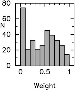
Figure 4: The distribution of ‘weights’ for the LMC RR1 variables in our sample. The weight is a measure of the probability that a star lies between the envelope lines of Figure 3. Our procedure for determining these weights is described in §2.1.

Our LMC data are the MACHO data for 330 RR Lyrae variables in 16 fields near the LMC bar. The observations were obtained between 1992 and 1999. The 330 stars that we analyse were all classified as bona fide RR1 variables by A04 who published their photometric and Fourier parameters. Figure 3 shows the $\phi_{31}-\log P$ plot for these stars, with the envelope lines for M3 superimposed. LMC variables with $\log P>-0.45$ (equivalent to $P=$ 0^d.355) have been excluded from the plot because M3 RR1 variables with periods greater than this appear to have evolved. In order to decide which of the LMC stars to include in our sample, we used a weighting scheme that Gladders & Yee (2000) devised for determining whether data points belong to a linear sequence, given their error. We constructed a Gaussian distribution for $\phi_{31}$ of each star, using a HWHM equal to the error listed by A04. Then we determined a ‘weight’ by measuring the fraction of the area under the Gaussian that fell between the envelope lines of Figure 3. Figure 4 shows the distribution of these weights. For our analysis, we will include only the stars with the highest probablility of fitting the M3 $\phi_{31}-\log P$ plot, i.e. the ones with weight greater than $0.5$.

2.2 The Crowded Stars

2.2.1 Correction for crowding

The period-$V$ amplitude relation for the M3-like RR1 variables in the LMC is shown in Figure 5 with the envelope lines from Figure 2 superimposed. Of the 147 stars plotted, 71 lie below the lines, 54 lie between them and 22 are above. If our hypothesis that low amplitudes are caused by blending is correct, we would expect the stars below the lines to be brighter. However, before we proceed to test this hypothesis, we need to consider the stars with the shortest periods ($\log P<-0.54$, i.e. $P<$ 0^d.29). They all have low amplitudes and could therefore be the LMC counterparts of the M3 stars, V105, V178 and V203. Since their low amplitudes might be intrinsic, they are not suitable for our crowding test. We therefore exclude all LMC variables with $P<$ 0^d.29 from our analysis. This leaves 127 stars: 54 below the lines, 51 between and 22 above. The mean magnitudes for the stars in these three regimes are listed in Table 1. Each row represents a different threshold for the weights of the stars considered. We will base our discussion on all of the stars with weight $>0.5$.

The data of Table 1 demonstrate that the stars that lie below the M3 period-amplitude relation are brighter than the ones that lie between the lines. This is the result we expect if the low amplitude stars are blended. A t-test (for all the stars with weight $>0.5$) indicates that the difference in $\langle V\rangle$ is highly significant, with a probability of only $0.0056$ that the two groups of stars are drawn from the same population. As for the stars that lie above the M3 lines, the difference between their mean $\langle V\rangle$ and that of the stars between the lines is not significant. Two M3 counterparts to these stars, V85 and V177, are displaced with respect to the other RR1 variables in the period-amplitude relation, but their $\phi_{31}$ and $\langle V\rangle$ values do not set them apart. CCC classified them with their long period/high luminosity group. We therefore suggest that these high amplitude stars are evolved, even though they do not appear brighter than the others.

Thus we can account for the relative mean magnitudes of the stars below, between and above the lines in Figure 5. In this discussion, we have not taken the effect of interstellar extinction into account and we know that it may vary from star to star. However, if the average extinction among the stars in each of the three regimes of Figure 5 is the same, the ranking of their mean $\langle V\rangle$ values should be correct.

Table 1 indicates that the $V$ magnitudes of 54 of 127 M3-like RR1 variables appear to be altered by crowding. This represents approximately 40% of the stars.

2.2.2 Crowding Simulations

If the RR1 stars that lie below the envelope lines in the period-amplitude diagram have unresolved companions, what are the apparent magnitudes of these companions? To answer this question, we performed simulations to ascertain how the presence of an unresolved companion would affect the observed magnitude and amplitude. A few examples of these simulations are presented in Table 2. The simulations show the change in $V$ magnitude and amplitude when an RR1 variable with $V=19.4$ or $19.7$ mag is blended with a star with $V=20-22$ mag. This range of $V$ magnitudes was selected for the companions because the LMC color magnitude diagram plotted by Alcock et al. (2000a) shows a high density of main sequence stars with $V>20$ mag and therefore the RR Lyrae are probably blended with stars like these. In Table 3, we show simulated data for three stars that are displaced from the central line in Figure 5 by more than $0.1$ mag. According to the table, the ‘true’ magnitudes of these RR Lyrae stars could be $V=19.70$, $19.56$ and $19.63$ while their unresolved companions have $V$ magnitudes, $21.25$, $20.28$ and $20.50$ respectively. These RR Lyrae $V$ magnitudes are typical LMC RR1 magnitudes and the $V$ magnitudes of the companions are consistent with LMC main sequence stars that belong to a younger population. RR Lyrae variables belong to an old population for which the main sequence turn-off is about $3.4$ mag fainter than the horizontal branch. Thus older main sequence stars would be too faint to have much of an effect.

The MACHO CM diagram also shows a high concentration of RR Lyrae variables and horizontal branch red clump stars with $V\sim 19.2$ mag, but we do not expect the stars in our data set to be blended with stars this bright. LMC RR Lyrae variables that have unresolved companions with $V\sim 19.2$ mag would be brighter than 19th magnitude. Such stars are known to exist in the MACHO database, but the 147 stars in our sample are fainter. In an independent study of LMC RR Lyrae variables, Di Fabrizio et al. (2005, hereafter referred to as DF05) identified five stars that could be blended with red clump stars among the RR Lyrae stars in their sample. These five stars had typical RR Lyrae periods, but small amplitudes and bright mean $V$ ($<19$) magnitudes. They concluded that one of these anomalous stars was an RR0 blended with a young main sequence star, but did not assign a definite classification to the other four.

2.3 The Extinction

A serious difficulty in deriving the distance to LMC stars is that the amount of interstellar extinction is not constant. Schwering & Israel (1991) estimated that the foreground extinction due to dust in the Galaxy ranges from $E(B-V)=0.07$ to $0.17$ over the LMC surface. Furthermore Harris et al. (1997) concluded that the distribution of dust within the LMC itself is clumpy. Therefore it is desirable to derive the extinction for the stars individually and we are in a position to do this. Since we have selected M3-like stars for our investigation, we can calculate the temperature of each star individually and then derive its reddening. We use CCC’s M3 period-temperature relation:

$$A=13.353-1.19\log P_{0}-4.058\log T_{eff}.$$ (1)

CCC found that a value of $A=-1.82\pm 0.03$ gave the best fit for the unevolved variables, but it predicted temperatures that were too low for stars that had evolved away from the ZAHB. Assuming that $A=-1.82$ and that $\log P_{0}=\log P_{1}+0.127$, we derive the following equation for calculating the temperatures of the unevolved LMC stars:

$$\log T_{eff}=3.702-0.293\log P_{1}.$$ (2)

The unreddened color $(V-R)_{0}$ can be computed from a relation derived by Kovács & Walker (1999) based on the models of Castelli, Gratton & Kurucz (1997a):

$$\log T_{eff}=3.8997-0.4892(V-R)_{0}+0.0113\log g+0.013\rm{[M/H]}$$ (3)

For this calculation, we assume that [M/H] = $-1.3$, the value adopted by CCC for their M3 study, and $\log g=2.93$, the mean of the $\log g$ values they calculated for the 15 stars in our reference sample. In order to calculate the corrected magnitudes $V_{0}$, we assume a ratio of total to selective absorption:

$$A_{V}/E(V-R)=5.35$$ (4)

(Schlegel, Finkbeiner & Davis 1998).

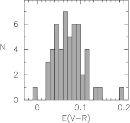
Figure 6: A histogram of E(V-R) for the 51 uncrowded, unevolved M3-like RR1 variables in 16 MACHO fields in the LMC. These are the stars that lie between the envelope lines of Figure 5.

The $\langle V\rangle_{F}$ and $\langle R\rangle_{F}$ magnitudes, the $V$ extinction and corrected magnitudes $V_{0}$ for the 51 uncrowded, unevolved stars are listed in Table 4. Figure 6 shows the distribution of $E(V-R)$ for the stars that we consider to be uncrowded, unevolved M3-like RR1 variables. The mean is $0.073\pm 0.02$ which corresponds to $V$ band extinction of $0.39\pm 0.10$. This value can be compared with the LMC extinction that Zaritsky et al. (2004) derived using a different technique. They measured effective temperatures and line-of-sight extinction for millions of individual stars by comparing stellar atmosphere models with $U,B,V,I$ photometry. Then they constructed extinction maps for stars in two temperature ranges where the model fitting between temperature and extinction was least degenerate: $5500K\leq T_{E}<6500K$ (cool, older stars) and $12,000K\leq T_{E}<45,000K$ (hot, younger stars). They derived a mean $V$ absorption of $0.43$ mag for the cool stars and $0.55$ mag for the hotter stars. With temperatures in the range $\sim 6100$ to $7300K$, RR Lyrae variables are similar to their cool star group and the mean extinction we have derived agrees with theirs to within our quoted error. However, for the cool stars, Zaritsky et al. found a bimodal distribution which they attributed to the existence of a dust layer. This bimodal structure is not evident in our data, but our sample is several orders of magnitude smaller than theirs. A Shapiro-Wilk W test indicates that our data, plotted in Figure 6, do not deviate significantly from a normal distribution.

We can also compare our extinction with the values derived by C03 for their RR Lyrae investigation since the two LMC fields they observed overlap with MACHO fields 6 and 13. They derived $E(B-V)=0.116\pm 0.017$ for their field A and $0.086\pm 0.017$ for field B from the colors of the edges of the instability strip. The corresponding total $V$ extinction values are $0.36\pm 0.05$ and $0.27\pm 0.05$. The mean extinction we calculate for the 9 stars in MACHO field 6 is $0.35$ mag and for the 4 stars in field 13, it is $0.38$. These are in good agreement with the extinction C03 derived for their field A and a bit high compared to their field B value, but still within the quoted errors.

We have pointed out that equation (2) predicts temperatures that are too low for stars that have evolved away from the ZAHB. Thus if the stars above the lines in Figure 5 have evolved, we would expect the extinction derived from equations (2), (3) and (4) to be underestimated and this would lead to faint $V_{0}$ values. This is exactly what we see in Table 5 where we list the mean $V_{0}$ these equations predict. Even though their mean $\langle V\rangle$ is comparable to the mean for the stars between the lines, their $V_{0}$ is $0.08$ mag fainter. We conclude that this supports our hypothesis that these stars have evolved. We will not include them in the sample of unevolved M3-like RR1 variables we use to determine the LMC distance. For the stars below the lines of Figure 5, equation (2) should be valid for computing temperatures, but if they are blended with other stars, their observed $(V-R)$ colors are not their true ones. Thus the $V_{0}$ values we derive for these stars individually will also be in error. However, if the mean extinction for these stars is comparable to the mean extinction for the stars between the lines, they will still appear brighter and this is what Table 5 illustrates.

2.4 Tilt Correction and Line-of-Sight Distribution

The distribution of the RR Lyrae population in the LMC has not been well established. Kinematic studies by Freeman et al. (1983), Storm et al. (1991) and Schommer et al. (1992) all indicated that the oldest globular clusters belong to a flattened disk-like system with $\sigma_{RV}\sim 28\rm{kms}^{-1}$. There was no evidence for the presence of a halo. It was therefore assumed that the RR Lyrae variables must belong to a disk population. However, van den Bergh (2004) pointed out that the observed radial velocities did not rule out the possibility that the globular clusters formed in a halo. Subsequently, radial velocities of LMC RR Lyrae variables derived by Minniti et al. (2003) and by Borissova et al. (2006) have indicated a larger velocity distribution ($\sigma_{RV}=50\pm 2\rm{kms}^{-1}$) and these authors argue that there is an old and metal poor halo in the LMC. If the RR Lyrae variables belong to a halo population, they should be distributed spherically with respect to the LMC center. On the other hand, if they belong to a disk population, the tilt of its plane with respect to the plane of the sky is an effect that must be considered when deriving the distance.

We made tilt corrections based on recent investigations of the LMC geometry by van der Marel & Cioni (2001) and by Nikolaev et al. (2004). Van der Marel & Cioni (2001) analysed the variations in brightness of asymptotic and red giant branch stars in near-IR color magnitude diagrams extracted from the DENIS and 2MASS surveys. They found a sinusoidal variation in apparent magnitude as a function of position angle, which they interpreted to be the result of distance variations because one side of the LMC plane is closer to us than the other. For their analysis, they assumed that the LMC center is located at $\alpha_{0}=82\mathrel{\raise 3.87495pt\hbox{$\circ$}\mkern-7.0mu\lower 1.72218pt\hbox{$\cdot$}}25$ and $\delta_{0}=-69\mathrel{\raise 3.87495pt\hbox{$\circ$}\mkern-7.0mu\lower 1.72218pt\hbox{$\cdot$}}5$ (van der Marel 2001) and included stars with $\rho$ in the range $2\mathrel{\raise 3.87495pt\hbox{$\circ$}\mkern-7.0mu\lower 1.72218pt\hbox{$\cdot$}}5-6\mathrel{\raise 3.87495pt\hbox{$\circ$}\mkern-7.0mu\lower 1.72218pt\hbox{$\cdot$}}7$ where $\rho$ is the angular distance from the LMC center. They derived an inclination angle $i=34\mathrel{\raise 3.87495pt\hbox{$\circ$}\mkern-7.0mu\lower 1.72218pt\hbox{$\cdot$}}7\pm 6\mathrel{\raise 3.87495pt\hbox{$\circ$}\mkern-7.0mu\lower 1.72218pt\hbox{$\cdot$}}2$ and line-of-nodes position angle $\Theta=122\mathrel{\raise 3.87495pt\hbox{$\circ$}\mkern-7.0mu\lower 1.72218pt\hbox{$\cdot$}}5\pm 8\mathrel{\raise 3.87495pt\hbox{$\circ$}\mkern-7.0mu\lower 1.72218pt\hbox{$\cdot$}}3$. Nikolaev et al. (2004) carried out a similar analysis based on more than 2000 MACHO Cepheids with $\rho<4^{\circ}$. Assuming $\alpha_{0}=79\mathrel{\raise 3.87495pt\hbox{$\circ$}\mkern-7.0mu\lower 1.72218pt\hbox{$\cdot$}}4$ and $\delta_{0}=-69\mathrel{\raise 3.87495pt\hbox{$\circ$}\mkern-7.0mu\lower 1.72218pt\hbox{$\cdot$}}03$, they derived $i=30\mathrel{\raise 3.87495pt\hbox{$\circ$}\mkern-7.0mu\lower 1.72218pt\hbox{$\cdot$}}7\pm 1\mathrel{\raise 3.87495pt\hbox{$\circ$}\mkern-7.0mu\lower 1.72218pt\hbox{$\cdot$}}1$ and $\Theta=151\mathrel{\raise 3.87495pt\hbox{$\circ$}\mkern-7.0mu\lower 1.72218pt\hbox{$\cdot$}}0\pm 2\mathrel{\raise 3.87495pt\hbox{$\circ$}\mkern-7.0mu\lower 1.72218pt\hbox{$\cdot$}}4$.

We used the equations listed in §2 of van der Marel & Cioni’s paper to calculate corrected $V_{0}$ magnitudes for both inclinations and they are listed in columns (7) and (8) of Table 4. Figure 7 shows the distribution of $V_{0}$ based on the three different assumptions for the LMC tilt. All three show a peak at approximately $19.0$ mag. Some of the dispersion in $V_{0}$ is due to depth within the LMC, but we expect a dispersion in absolute magnitude as well because our M3 reference stars have a range of $0.2$ in apparent magnitude. The normal parameter estimates are listed in Table 6. A Shapiro-Wilk W test indicates that none of the three deviates significantly from a normal distribution.

We adopt the tilt corrections based on the viewing angles derived by Nikolaev et al. because the stars in their sample, like ours, are all within $4^{\circ}$ of the LMC center. The mean $V_{0}$ based on these viewing angles is exactly the same as the value obtained when no tilt correction is applied. Therefore our derived $V_{0}$ does not depend on any assumption about the distribution of the LMC RR Lyrae variables.

3 The LMC Distance

3.1 The Apparent Magnitude of the RR1 Variables

We have adopted a mean $V_{0}=19.02$ for the 51 uncrowded, unevolved M3-like RR1 variables, based on the LMC viewing angles derived by Nikolaev et al. (2004). Since our mean magnitudes are the $A_{0}$ values from equation (5), we need to convert them to intensity means before we compute an LMC distance. A04 showed that the intensity means are $\sim 0.01$ mag brighter than $A_{0}$ so we revise our adopted mean $V_{0}$ to $19.01$ mag.

To determine the precision of the $V_{0}$ values listed in Table 4, we need to consider the errors in reddening and the errors in the calibration of our photometry. We have already pointed out in §2.3 that the error in $E(V-R)$ is $0.018$ mag which corresponds to $0.10$ mag in the $V$ exinction. Our calibrated $V$ and $R$ magnitudes are from the study by A04, and were calculated from transformation equations derived by Alcock et al. (1999), designated calibration version 990318. They derived an internal precision of $\sigma_{V}=0.021$ for their $V$ magnitudes by comparing the results for stars in overlapping (MACHO) fields.

Another way to test our calibration is to compare with the results from other investigations. Two of the 51 uncrowded, unevolved M3-like RR1 stars that we have listed in Table 4 were observed by DF05. The mean (intensity) magnitudes derived from the two studies for these stars are listed in Table 7 and they agree to within $0.01$ mag. In our earlier paper (A04), we listed mean magnitudes for five additional RR1 stars that were observed by both groups and the MACHO magnitudes were significantly brighter. However, in our new analysis, we have classified two of these stars as crowded. Their mean magnitudes are also listed in Table 7 and it is clear that the MACHO magnitudes are brighter than the ones derived by DF05. The remaining three are not M3-like so we can not ascertain whether or not they are crowded.

DF05 also compared their $V$ magnitudes with MACHO data provided by Alves and by Kovács (Alcock et al 2003) and found that the MACHO magnitudes were approximately $0.04$ mag brighter on average. DF05 concluded that the difference occurred because the MACHO reduction procedure did not adequately compensate for crowding in stars with $V>18.25$. The MACHO collaboration recognized the crowding problem so A04 made crowding corrections by adding artifical stars of known magnitude to the the image frames and measuring $\Delta V$ the difference between their input and recovered magnitudes. However, these corrections introduce a relatively large error of $\sim 0.10$ mag into the adopted apparent magnitudes. In the present investigation, we have dealt with this problem by identifying crowded stars and removing them from our data set.

We can not determine which of the MACHO stars in the Alves and Kovács samples were crowded; however, our sample of M3-like stars can provide some insight. According to the data listed in Table 1, approximately 40% of the M3-like variables are crowded and as a consequence, their average $V$ magnitude is $0.09$ mag brighter. If we assume that the mean MACHO magnitude for 40% of the stars in the data sets that Alves and Kovács provided to DF05 is $0.09$ mag brighter (as a result of blending with main sequence stars), while the remaining 60% have $V$ magnitudes similar to the ones that DF05 derived, we would expect the MACHO stars to be about $0.04$ mag brighter on average. Thus if the crowded stars could be removed from the MACHO sample, the photometry derived in these two independent studies would be in good agreement.

Since our $V$ photometry for uncrowded stars appears to be in good agreement with that of DF05, we assume that the uncertainty in our calibrated $V$ magnitudes is $0.02$ mag. Therefore we adopt $V_{0}=19.01\pm 0.10$ (extinction) $\pm 0.02$ (calibration) for our sample of uncrowded, unevolved M3-like variables in the LMC. This is in good agreement with the result of C03: $V_{0}=19.064\pm 0.064$ at [Fe/H]$=-1.5$ on the metallicity scale of Harris (1996). Taking into account the fact that the RR1 variables in our sample are M3-like, that [Fe/H] for M3 is $-1.57$ on the Harris scale and that C03 derived $\Delta M_{V}/\Delta\rm{[Fe/H]}=0.214$ for the RR Lyrae variables in the LMC, we estimate that $V_{0}=19.05$ at [Fe/H]$=-1.57$ for the data of C03.

3.2 The Absolute Magnitude and Distance of the RR1 Variables

A major challenge in determining the LMC distance is to identify a homogeneous group of stars for which the absolute magnitude is well established. We deal with this problem by using the M3 distance modulus to calculate the absolute $V$ magnitude of our 15 M3 reference stars. Then we assume that the uncrowded stars in our LMC sample have the same mean $M_{V}$. The M3 distance modulus has been derived in investigations of RR Lyrae variables by Marconi et al. (2003) and by Sollima et al. (2006).

Taking a theoretical approach, Marconi et al. applied pulsation theory to the $BV$ observations of M3 by Corwin & Carney (2001) and the $K$ observations of Longmore et al. (1990). They compared the results from pulsation theory with the observed edges of the instability strip, the observed $K$ band period-magnitude relation and the observed relations among period-magnitude-color and period-magnitude-amplitude. For their calculations, they used bolometric corrections and temperature-color transformations provided by Castelli, Gratton & Kurucz (1997a, 1997b) and adopted a mean RR Lyrae mass of $0.67{M_{\odot}}$, based on evolutionary models of Cassisi et al. (2004). They computed a mean distance modulus $DM=15.07\pm 0.05$, but pointed out that if they had used the models of Vandenberg et al. (2000) instead, $DM$ would have been $15.05$. We adopt the distance modulus based on the Cassisi models, DM=$15.07\pm 0.05$. Our 15 M3 reference stars have $V$ magnitudes ranging from $15.48$ to $15.68$ with mean $\langle V\rangle=15.60$. If we apply CCC’s extinction, $E(B-V)=0.01\pm 0.01$, this corresponds to $V_{0}=15.57$ which leads to $M_{V}=0.50\pm 0.06$.

Sollima et al. derived an M3 distance modulus from the RR Lyrae period-metallicity-$K$ band luminosity $(PL_{K})$ relation that they calibrated from observations:

$$M_{K}=-2.38(\pm 0.04)\log P_{F}+0.08(\pm 0.11)\rm{[Fe/H]}-1.05(\pm 0.13)$$ (6)

where $M_{K}$ is the absolute $K$ magnitude, $P_{F}$ is the fundamentalized pulsation period and [Fe/H] refers to the metallicity scale of Carretta & Gratton (1997). They derived their coefficient of $\log P_{F}$ from the slope of the $K-\log P_{F}$ relation for 538 RR Lyrae variables in 16 globular clusters and their [Fe/H] coefficient from the slope of the $(M_{K}-2.38\log P)$ - [Fe/H] relation for the four globular clusters in their sample that had distance determinations based on Hipparcos trig parallaxes for local subdwarfs. They obtained their zero point from the $K$ magnitude of RR Lyrae combined with the trig parallax that Benedict et al. (2002) measured for it from HST astrometry. From equation (6), Sollima et al. calculated an M3 distance modulus of $15.07$. Thus $M_{V}=0.50\pm 0.20$.

Unfortunately, the large error in the coefficient of [Fe/H] in equation (6) results in a large uncertainty in $M_{K}$. Therefore it seems appropriate to calculate the M3 distance modulus directly from the absolute magnitude that Benedict et al. derived for RR Lyrae: $M_{V}=0.61^{-0.11}_{+0.10}$. The [Fe/H] for RR Lyrae is $-1.39$ (Clementini et al. 1995), which is comparable to the M3 metal abundance, $-1.34$ on the scale of Carretta & Gratton. Furthermore, the pulsation period of RR Lyrae, 0^d.567, and its maximum $V$ amplitude which is $0.9$ mag according to Smith et al. (2003) places it on the M3 period-amplitude relation. CCC studied five RR0 stars with periods within $0.01$ days of 0^d.567 (V10, V69, V135, V137 and V142). The mean $V$ amplitude for these stars is $0.89$ mag and their mean $\langle V\rangle$ is $15.65\pm 0.02$. Assuming that their mean absolute magnitude is the same as that of RR Lyrae, we derive a mean $M_{V}=0.56\pm 0.11$ for our 15 M3 reference stars.

The Baade-Wesselink technique has not been applied to any RR Lyrae variables in M3. However, in a review of RR Lyrae luminosities, Cacciari (2003) reported the result of a B-W analysis for the star RR Cet which has a metal abundance comparable to that of M3. Cacciari et al. (2000) derived $M_{V}=0.56\pm 0.15$ for this star which, with a period of 0^d.553 and $V$ amplitude $0.98$ mag (Simon & Teays 1982) fits the M3 P-A relation. Six stars analysed by CCC (V36, V40, V71, V89, V133 and V149) have periods within $0.01$ days of 0^d.553 and the mean $V$ amplitude and mean $\langle V\rangle$ they derived for these stars were $0.99$ and $15.65$ respectively. By comparing the mean magnitudes of these six stars with those of our 15 M3 reference stars, we derive mean $M_{V}=0.52\pm 0.15$ for the reference stars.

The mean of our four $M_{V}$ values is $0.52$ with a standard deviation $0.02$ mag. Combining this with the $V_{0}=19.01\pm 0.10$ (extinction error) $\pm 0.02$ (calibration error) that we derived for the uncrowded, unevolved M3-like RR1 variables in our LMC sample and adding the estimated errors in quadrature, leads to distance modulus $\mu_{LMC}=18.49\pm 0.11$.

Our distance modulus is in good agreement with $\mu_{0}=18.48\pm 0.08$ derived by Borissova et al. (2004) from $K$-band photometry of 37 RR Lyrae variables in the inner regions of the LMC. In their investigation, they derived a mean $\langle K\rangle=18.20$ and assumed that the mean $K$ band absorption $A_{K}=0.05$ mag. By following the procedure described by Bono et al. (2001, 2003), they calculated $M_{K}=-0.332$ at $\log P=-0.30$. Their adopted absolute $K$ magnitude was $0.85$ mag brighter than our adopted $M_{V}$. This is consistent with the apparent magnitudes we have derived; their mean $K_{0}$ ($18.15$) is $0.86$ mag brighter than our $V_{0}$, $19.01$. Our adopted $\mu_{0}$ is also comparable to the value $(18.48)$ obtained by McNamara et al. (2007) in their recent analysis of $\delta$ Scuti stars.

By identifying the crowded stars and removing them from the sample, we have avoided using the crowding corrections that introduced an additional uncertainty of $0.10$ mag to the distance modulus we derived in our earlier study (A04). The main source of error in this investigation is the error in estimating the $V$ extinction.

4 Summary

We have devised a new method for identifying crowded RR1 variable stars in the LMC, based on simulations that show that stars with unresolved companions have low amplitudes for their periods. Given that many LMC RR Lyrae variables have properties similar to the ones in the Galactic globular cluster M3, we used the M3 $\phi_{31}-\log P$ relation to identify the M3-like unevolved RR1 variables in our LMC sample. The Fourier phase parameter $\phi_{31}$ is useful for selecting a homogeneous sample because it is not affected by crowding.

When the M3-like variables were plotted on the M3 period-amplitude diagram, we found that the mean $V$ magnitude of the LMC stars with low amplitudes was $0.09$ mag brighter than the mean for the stars that fit the M3 period-amplitude relation. Four of the stars in our sample were observed in the study of LMC RR Lyrae variables by DF05. Comparing the photometry from the two studies, we found that our $V$ magnitudes for the two stars considered to be uncrowded agreed to within $0.01$ mag, while the MACHO $V$ magnitudes for the two stars we considered to be crowded were more than $0.05$ mag brighter. From this, we conclude that our method for identifying crowded RR Lyrae variables is effective. It could prove to be useful for identifying crowded RR Lyrae variables in other local group galaxies.

We used the M3 period-temperature relation for unevolved RR Lyrae variables to determine the temperature and reddening for each of the uncrowded RR1 variables in our sample. After making corrections for the tilt of the LMC, we derived a mean $V_{0}$ magnitude of $19.01\pm 0.10$ (extinction) $\pm 0.02$ (calibration). Then to estimate the absolute magnitude, we used the M3 distance modulus and the trig parallax of RR Lyrae to derive the mean absolute magnitude of the unevolved RR1 variables in our M3 reference sample. This turned out to be $M_{V}=0.52\pm 0.02$.

Finally, we derived an LMC distance modulus $\mu_{LMC}=18.49\pm 0.11$ which is in good agreement with the results of other recent studies and with $18.5$ mag, the value employed by the Hubble Space Telescope’s key project for measuring the Hubble constant (Freedman et al. 2001).

Figure 1: Plot of $\phi_{31}$ vs. $\log P$ for the RR1 variables in four well studied Galactic globular clusters: the Oosterhoff type I clusters M107 (open circles), M5 (solid circles) and M3 (open triangles) and the Oosterhoff type II cluster M68 (solid triangles). The $\phi_{31}$ values plotted here for these four clusters were determined by Clement & Shelton (1997), Kaluzny et al. (2000), Cacciari et al (2005) and Walker (1994) respectively. Their metal abundances are $-1.10$, $-1.32$, $-1.50$ and $-2.43$ on the $\rm{Fe}_{\rm{II}}$ metallicity scale of Kraft & Ivans (2003).

Figure 2: Plots of $\phi_{31}$, $V$ amplitude and the (intensity) mean $V$ magnitude versus $\log P$ for the 15 M3 unevolved RR1 variables that we include in our sample. The data are taken from the investigation by CCC. In the two upper panels, the central lines represent least squares fits to the data and the outer lines, plotted with the same slope, are the envelope lines that encompass all of the data.

Figure 3: A plot of the Fourier phase difference $\phi_{31}$ vs $\log P$ for 330 bona fide RR1 variables in 16 MACHO fields in the LMC. The superimposed lines represent the $\phi_{31}-\log P$ relation for the M3 RR1 variables studied by CCC. (See the upper panel of Figure 2.)

Figure 5: The period-$V$ amplitude relation for the M3-like RR1 variables in 16 MACHO fields in the LMC. Only the 147 stars with weight greater than $0.5$ in Figure 4 are included. The superimposed lines represent the period-amplitude relation for the M3 RR1 variables (see the centre panel of Figure 2).

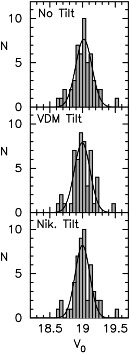
Figure 7: A histogram for the LMC variables that lie between the lines in Figure 5. These are the stars that we consider to be uncrowded M3-like unevolved RR1 variables. Three histograms are plotted: the first represents the data with no tilt correction and the other two include the tilt corrections of van der Marel & Cioni (2001) and Nikolaev et al. (2004) respectively. The curves are Gaussian fits to the data.

Table 1: Mean $\langle V\rangle$ and Location in the Period-Amplitude Diagram

Weight	Mean $\langle V\rangle$	N	Mean $\langle V\rangle$	N	Mean $\langle V\rangle$	N
	(below)		(between)		(above)
(1)	(2)	(3)	(4)	(5)	(6)	(7)
Wt. $\geq 0.5$	$19.31\pm 0.02$	54	$19.40\pm 0.02$	51	$19.43\pm 0.04$	22
Wt. $\geq 0.6$	$19.30\pm 0.02$	43	$19.40\pm 0.02$	33	$19.45\pm 0.05$	16
Wt. $\geq 0.7$	$19.28\pm 0.03$	31	$19.38\pm 0.02$	25	$19.37\pm 0.05$	8
Wt. $\geq 0.8$	$19.32\pm 0.03$	17	$19.35\pm 0.03$	13	$19.45\pm 0.06$	3
Wt. $\geq 0.9$	$19.31\pm 0.05$	9	$19.39\pm 0.03$	6	$19.40\pm 0.06$	2

Note. — The terms ‘below’, ‘between’ and ‘above’ refer to the location relative to the lines in Figure 5. The weights represent the probability that the stars lie between the envelope lines in Figure 3. Stars with $P<$0^d.29 are not included.

Table 2: Crowding Simulations

$V$	Amplitude	$V$	$V$	Amplitude
(RR)	(RR)	(Companion)	(Observed)	(Observed)
(1)	(2)	(3)	(4)	(5)
19.4	0.45	20.0	18.90	0.29
19.4	0.45	20.5	19.06	0.33
19.4	0.45	21.0	19.17	0.37
19.4	0.45	21.5	19.25	0.39
19.4	0.45	22.0	19.30	0.41
19.7	0.45	20.0	19.08	0.26
19.7	0.45	20.5	19.27	0.30
19.7	0.45	21.0	19.41	0.35
19.7	0.45	21.5	19.51	0.38
19.7	0.45	22.0	19.57	0.40

Note. — The simulated magnitudes listed in columns (1) and (3) combine to produce the magnitudes listed in column (4). Thus if an RR Lyrae variable with $V=19.4$ has an unresolved companion with $V=20.0$, its observed magnitude will be $V=18.90$. As a result of the blending, its original amplitude ($0.45$ mag) will be reduced to $0.29$ mag.

Table 3: Sample Magnitudes for Three Blended Stars

Star	$\log P$	Amplitude	$\langle V\rangle$	$\langle V\rangle$	Amplitude
		(observed)	(observed)	(RR + companion)	(true)
(1)	(2)	(3)	(4)	(5)	(6)
80.6475.3548	-0.486	0.36	19.46	19.70+21.25	0.45
80.6708.6879	-0.503	0.30	19.10	19.56+20.28	0.46
81.8398.799	-0.486	0.30	19.22	19.63+20.50	0.44

Note. — The simulated magnitudes listed in column (5) combine to produce the observed magnitudes of column (4). For example, our simulation implies that star $80.6475.3548$ is really an RR Lyrae with $V=19.70$ blended with an unresolved companion whose $V=21.25$ mag. As a result of the blending, the original $V$ amplitudes listed in column (6) are reduced to the observed amplitudes listed in column (3).

Table 4: Parameters of the Uncrowded, Unevolved M3-like RR1 Variables

Star	Period	$\langle V\rangle_{F}$	$\langle R\rangle_{F}$	Ext$(V)$	$V_{0}$	$V_{0}$(vdM)	$V_{0}$(Nik)	Weight
(1)	(2)	(3)	(4)	(5)	(6)	(7)	(8)	(9)
2.4789.946	0.326910	19.23	19.05	0.18	19.05	19.05	19.04	0.89
2.5150.896	0.337123	19.21	19.01	0.24	18.97	18.97	18.96	0.59
2.5151.982	0.344523	19.33	19.10	0.37	18.96	18.96	18.95	0.63
2.5269.422	0.318123	19.52	19.29	0.48	19.04	19.03	19.03	0.90
2.5511.772	0.302923	19.33	19.17	0.18	19.15	19.15	19.15	0.93
2.5633.1369	0.293763	19.30	19.13	0.27	19.03	19.03	19.03	0.71

Note. — The $V_{0}$ values are corrected for extinction; the $V_{0}$(vdM) and $V_{0}$(Nik) values are corrected for tilt as well, according to the LMC viewing angles derived by van der Marel & Cioni (2001) and by Nikolaev et al. (2004) respectively. The weight is the probability that the star lies between the envelope lines of Figure 3. Table 4 is presented in its entirety in the electronic edition of the Astronomical Journal. A portion is shown here for guidance regarding its form and content.

Table 5: Mean $V_{0}$ for Stars with Wt. $>0.5$

Location in	Mean $V_{0}$		N
Fig 5
Below the lines	$18.88\pm 0.02$		54
Between the lines	$19.02\pm 0.02$		51
Above the lines	$19.10\pm 0.05$		22

Note. — The $V_{0}$ values have been derived under the assumption that the stars’ temperatures can be computed from equation (2) and that their observed $(V-R)$ colors are correct. These two assumptions are valid for the stars that lie between the lines, but not for the others. This is discussed in the final paragraph of §2.3.

Table 6: Fitted Normal Parameter Estimates for Fig 7

Tilt correction	$\mu$	$\sigma$	N
None	19.02	0.16	51
van der Marel	19.00	0.15	51
Nikolaev	19.02	0.16	51

Table 7: Comparison with the DF05 Photometry

ID	Crowded?	$\langle V\rangle_{int}$	ID	$\langle V\rangle_{int}$
(MACHO)	(MACHO)	(MACHO)	(DF05)	(DF05)
6.7054.710	no	19.45	7864	19.46
13.5838.667	no	19.39	7648	19.38
6.6689.563	yes	19.23	2249	19.37
13.6079.604	yes	19.24	4749	19.31

References

- Alcock et al. (1996) Alcock, C. et al. 1996, AJ, 111, 1146
- Alcock et al. (1997) Alcock, C. et al. 1997, ApJ, 482, 89
- Alcock et al. (1999) Alcock, C. et al. 1999, PASP, 111, 1539
- (4) Alcock, C. et al. 2000a, AJ, 119, 2194
- (5) Alcock, C. et al. 2000b, ApJ, 542, 257
- Alcock et al. (2003) Alcock, C. et al. 2003, ApJ, 598, 597
- Alcock et al. (2004) Alcock, C. et al. 2004, AJ, 127, 334 (A04)
- Bailey (1913) Bailey, S. I. 1913, Harvard Ann. 78, 1
- Benedict et al. (2002) Benedict, G. F. et al. 2002, AJ, 123, 473
- Bono et al. (2001) Bono, G., Caputo, F., Castellani, V. Marconi, M. & Storm, J. 2001, MNRAS, 326, 1183
- Bono et al. (2003) Bono, G., Caputo, F., Castellani, V. Marconi, M., Storm, J. & Degl’Innocenti, S. 2003, MNRAS, 344, 1097
- Borissova et al. (2004) Borissova, J., Minniti, D., Rejkuba, M., Alves, D., Cook, K. H., & Freeman, K. C. 2004 A&A, 423, 97
- Borissova et al. (2006) Borissova, J., Minniti, D., Rejkuba, M., Alves, D. 2006 A&A, 460, 459
- Cacciari (2003) Cacciari, C. 2003, in New Horizons in Globular Cluster Astronomy, ed. G. Piotto, G. Meylan, S. G. Djorgovsli & M. Riello (ASP Conf. Ser. 296) (San Francisco: ASP), 329
- Cacciari et al. (2000) Cacciari, C., Clementini, G., Castelli, F. & Melandri, F. 2000, in IAU Colloq. 176, The Impact of Large-Scale Surveys on Pulsating Star Research, ed. L. Szabados & D. W. Kurtz (ASP Conf. Ser. 203) (San Francisco: ASP), 176
- Cacciari et al. (2005) Cacciari, C., Corwin, T. M. & Carney, B. W. 2005, AJ, 129, 267 (CCC)
- Carretta & Gratton (1997) Carretta, E. & Gratton, R. G. 1997, A&AS, 121, 95
- Cassisi et al. (2004) Cassisi, S., Castellani, M., Caputo, F. & Castellani, V. 2004, A&A, 426, 641
- (19) Castelli, F., Gratton, R. G. & Kurucz, R. L. 1997a, A&A, 318, 841
- (20) Castelli, F., Gratton, R. G. & Kurucz, R. L. 1997b, A&A, 324, 432
- Catelan (2004) Catelan, M. 2004, in IAU Colloq. 193, Variable Stars in the Local Group, ed. D. W. Kurtz & K. R. Pollard (ASP Conf. Ser. 310) (San Francisco: ASP), 113
- Clement et al. (2002) Clement, C. M., Muzzin, A. V., Rowe, J. F. & the MACHO Collaboration. 2002, BAAS, 34, 651
- Clement et al. (1985) Clement, C. M., Nemec, J. M., Robert, N., Wells, T., Dickens, R. J. & Bingham, E. A. 1985, AJ, 92, 825
- (24) Clement, C. M. & Shelton, I. 1997, AJ, 113, 1711
- Clementini et al. (1995) Clementini, G., Carretta, E., Gratton, R. G., Merighi, R., Mould, J. R. & McCarthy, J.K. 1995, AJ, 110, 2319
- Clementini et al. (2004) Clementini, G., Corwin, T. M., Carney, B. W. & Sumerel, A. N. 2004, AJ, 127, 938
- Clementini et al. (2003) Clementini, G., Gratton, R. G., Bragaglia, A., Carretta, E., Di Fabrizio, L. & Maio, M. 2003, AJ, 125, 1309 (C03)
- Corwin & Carney (2001) Corwin, T. M. & Carney, B.W. 2001, AJ, 122, 3183
- Corwin et al. (1999) Corwin, T. M., Carney, B.W. & Allen, D. M. 1999, AJ, 117, 1332
- Di Fabrizio et al. (2005) Di Fabrizio, L., Clementini, G., Maio, M., Bragaglia, A., Carretta, E., Gratton, R., Montegriffo, P. & Zoccali, M. 2005, A&A, 430, 603 (DF05)
- Freedman et al. (2001) Freedman, W. L. et al. 2001, ApJ, 553, 47
- Freeman et al. (1983) Freeman, K. C., Illingworth, G., & Oemler, A. Jr. 1983, ApJ, 272, 488
- Gladders & Yee (2000) Gladders, M. D. & Yee, H. K. C. 2000, AJ, 120, 2148
- Harris et al. (1997) Harris, J., Zaritsky, D., & Thompson, I. 1997, AJ, 114, 1933
- Harris (1996) Harris, W. E. 1996, AJ, 112, 1487
- Kaluzny et al. (1998) Kałużny, J., Hilditch, R. W., Clement, C., & Ruciński, S. M. 1998, MNRAS, 296, 347
- Kaluzny et al. (2000) Kałużny, J., Olech, A., Thompson, I., Pych, W., Krzemiński, W., & Schwarzenberg-Czerny, A. 2000, A&AS, 143, 215
- Kovács & Walker (1999) Kovács, G. & Walker, A. R. 1999, ApJ, 512, 271
- Kraft & Ivans (2003) Kraft, R. P. & Ivans, I.I. 2003, PASP, 115, 143
- Longmore et al. (1990) Longmore, A. J., Dixon, R., Skillen, I., Jameson, R. F., & Fernley, J. A. 1990, MNRAS, 247, 684
- McNamara et al. (2007) McNamara, D. H., Clementini, G. & Marconi, M. 2007, AJ, 133, 2752
- Marconi et al. (2003) Marconi, M., Caputo, F., Di Criscienzo, M. & Castellani, M. 2003, ApJ, 596, 299
- Minniti et al. (2003) Minniti, D., Borissova, J., Rejkuba, M., Alves, D. R., Cook, K. H., & Freeman, K.C. 2003, Science, 301, 1508
- Nikolaev et al. (2004) Nikolaev, S., Drake, A. J., Keller, S. C., Cook, K. H., Dalal, N., Griest, K., Welch, D. L., & Kanbur, S. M. 2004, ApJ, 601, 260
- Schlegel et al. (1998) Schlegel, D. J., Finkbeiner, D. P. & Davis, M. 1998, ApJ, 500, 525
- Schommer et al. (1992) Schommer, R. A., Olszewski, E. W., Suntzeff, N. B. & Harris, H. C. 1992, AJ, 103, 447
- Schwering & Israel (1991) Schwering, P. B. W. & Israel, F. P. 1991, A&A, 246, 231
- Simon & Clement (1993) Simon, N. R. & Clement, C. M. 1993, ApJ, 410, 526
- Simon & Lee (1981) Simon, N. R. & Lee, A. S. 1981, ApJ, 248, 291
- Simon & Teays (1982) Simon, N. R. & Teays, T. J. 1982, ApJ, 261, 586
- Sollima et al. (2006) Sollima, A., Cacciari, C. & Valenti, E. 2006, MNRAS, 372, 1675
- Smith et al. (2003) Smith, H. A. et al. 2003, PASP, 115, 43
- Storm et al. (1991) Storm, J., Carney, B. W., Freedman, W. L., & Madore, B. F. 1991, PASP, 103, 261
- Szeidl (1988) Szeidl, B. 1988, in Multimode Stellar Pulsations, ed. G. Kovács, L. Szabados, & B. Szeidl (Budapest: Konkoly Obs.), 45
- van den Bergh (2004) van den Bergh, S. 2004, AJ, 127, 1897
- Vandenberg et al. (2000) Vandenberg, D. A., Swenson, F. J., Iglesias, C. A., & Alexander, D. R. 2000, ApJ, 532, 430
- van der Marel (2001) van der Marel, R. P. 2001, AJ, 122, 1827
- van der Marel & Cioni (2001) van der Marel, R. P. & Cioni, M. L. 2001, AJ, 122, 1807
- Walker (1994) Walker, A. R. 1994, AJ, 108, 555
- Walker, A. R. & Nemec (1996) Walker, A. R. & Nemec, J. M. 1996, AJ, 112, 2026
- Zaritsky et al. (2004) Zaritsky, D., Harris, J., Thompson, I. B. & Grebel, E. K. 2004, AJ, 128, 1606