VLT / Infrared Integral Field Spectrometer Observations of Molecular Hydrogen Lines in the Knots in the Planetary Nebula NGC 7293 (the Helix Nebula)

Abstract

Knots are commonly found in nearby planetary nebulae (PNe) and star forming regions. Within PNe, knots are often found to be associated with the brightest parts of the nebulae and understanding the physics involved in knots may reveal the processes dominating in PNe. As one of the closest PNe, the Helix Nebula (NGC 7293) is an ideal target to study such small-scale ($\sim$300 AU) structures. We have obtained infrared integral spectroscopy of a comet-shaped knot in the Helix Nebula using SINFONI on the Very Large Telescope at high spatial resolution (50–125 mas). With spatially resolved 2 $\mu$m spectra, we find that the H₂ rotational temperature within the cometary knots is uniform. The rotational-vibrational temperature of the cometary knot (situated in the innermost region of the nebula, 2.5 arcmin away from the central star), is 1800 K, higher than the temperature seen in the outer regions (5–6 arcmin from the central star) of the nebula (900 K), showing that the excitation temperature varies across the nebula. The obtained intensities are reasonably well fitted with 27 km s^-1 C-type shock model. This ambient gas velocity is slightly higher than the observed [HeII] wind velocity of 13 km s^-1. The gas excitation can also be reproduced with a PDR (photo dominant region) model, but this requires an order of magnitude higher UV radiation. Both models have limitations, highlighting the need for models that treats both hydrodynamical physics and the PDR.

1 Introduction

In recent years it has become clear that knots of dense material are common in nebulae, including Planetary Nebulae (PNe; e.g. O’Dell et al., 2002) and star-forming regions (e.g. McCaughrean & Mac Low, 1997). In the one of the best studied PN case, that of the Helix Nebula (NGC 7293), knots in the inner regions have a comet-like shape (O’Dell & Handron, 1996) and are thus known as cometary knots. The Helix nebula is estimated to contain more than 20,000 cometary-shaped knots (Meixner et al., 2005). The apparent commonality of occurrence in PNe of these knots has lead to the assertion that all circumstellar nebulae are clumpy in structure (e.g. O’Dell et al., 2002; Speck et al., 2002; Matsuura et al., 2005b). As knots occupy the brightest parts of the planetary nebulae, understanding their physical nature is essential to understanding the dominant physics governing the nebula.

The origin of these knots remains unknown. When the knots form is also disputed: they may have been present during the preceding AGB (Asymptotic Giant Branch) phase (e.g. Dyson et al., 1989), or only have formed during the PN phase. The suggested formation mechanisms fall into two main scenarios. Firstly, photo-evaporation from condensations which pre-exist in the circumstellar envelope were considered. Speck et al. (2002) suggest that the UV radiation from the central star heats the surface of a condensation, emitting H$\alpha$ and H₂ on the facing side. Secondly, the interaction of a fast stellar wind with the slowly expanding AGB wind, during the early stage of PN phase, has been considered (e.g Vishniac, 1994; Pittard et al., 2005; García-Segura et al., 2006). Pittard et al. (2005) found that cometary knots may be formed through instabilities where a supersonic wind impacts a subsonic wind.

In addition to being seen as inhomogeneities within the ionized gas emission from nebulae, the knots also contain molecular gas (Speck et al., 2002, 2003). This yields a potential clue to their origin. Redman et al. (2003) argued that some molecular species formed in the AGB atmosphere can survive if molecules are shielded in clumps from UV radiations by extinction. But if the knots (re-)form during the ionized PN phase, the earlier AGB molecules were photo-dissociated, and the molecules reform within the knots, under conditions of relatively low density and higher UV intensity compared to the AGB wind. In these conditions only simple molecules are expected to be present (Woods, 2004).

Using seeing-limited observations (1.2 arcsec) of the H₂ v=1–0 S(1) line in a single knot, Huggins et al. (2002) found H₂ gas in both the head and the tail of the knot, following the distribution of ionised gas traced by H$\alpha$ and [NII]. In contrast, CO thermal emission was found to emanate only from the tail. Higher angular resolution images obtained with HST (Meixner et al., 2005) resolved the globular H₂ emission into crescent-shaped regions. With these previous studies, it is not clear whether the hydrogen molecules and ionised gas are co-located within the head or spatially separated.

The excitation mechanisms for molecular hydrogen in planetary nebula have long been controversial, with contention between fluorescent/thermal excitation in photon-dominant regions (PDR) or shock excitation. Tielens & Hollenbach (1985) and Black & van Dishoeck (1987) showed that vibrationally excited H₂ (by FUV pumping) traces the surface of dense regions in the process of becoming photo-ionised. On the other hand, molecules can form in a post-shock region (Neufeld & Dalgarno, 1989), and H₂ can be excited by shocks (Beckwith et al., 1980; Hollenbach & McKee, 1989). The cooling region after the shock can be resolved if it is C-type (continuous) shock, but the region is too small to be resolved for J-type (jump) shocks. A comparison of models with spatially resolved spectra, which covers multiple line ratios, will help understanding the excitation mechanism of H₂.

The Helix Nebula (NGC 7293) is one of the nearest PNe, with a largest diameter of more than half a degree (Hora et al., 2006) and a parallax distance of 219 pc (Harris et al., 2007). Because of its distance, small-scale structures inside the nebula are well resolved and this nebula is used as a proxy to understand the structures found in PNe.

We have observed a cometary knot in the Helix Nebula, using the adaptive-optics-assisted, near-infrared integral field spectrometer on the Very Large Telescope. We have achieved 50–100 mas spatial resolution. Our data provide the first spatially resolved spectra within a knot at 2 $\mu$m and further this is the highest spatial resolution image+spectra of this PN at this wavelength. Our observations of H₂ spectral line ratios allow us to derive the excitation temperatures within the knot, as well as differentiation between the possible excitation mechanisms of H₂.

2 Observations and Analysis

Table 1: Observing log

Target					Telluric Standard
		Pixel scale of the camera	Pixel scale in reduced data	Exp†	Name	Spec	K-mag‡
		mas2	mas2
K1		125$\times$250	125$\times$125	300s$\times$10	Hip 115329	G2V	7.552$\pm$0.017
				600s$\times$10
		50$\times$100	50$\times$50	600s$\times$10	Hip 023422	G2V	7.862$\pm$0.017

A knot in the Helix Nebula was observed by the Spectrograph for INtegral Field Observations in the Near Infrared (SINFONI; Eisenhauer et al., 2003; Bonnet et al., 2004) installed at the Cassegrain focus of the Very Large Telescope. The grating for the K-band was used. The wavelength band of the grating was mapped to the 2048 pixel detector in the dispersion direction. We used two plate-scales: the spatial resolutions are 125$\times$250 mas² and 50$\times$100 mas². For all of the observations, a nearby star (RA=22:29:33.017 Dec=$-$20:48:12.68) was used as Adaptive Optics (AO) guide star. The spatial resolution is usually determined by the pixel scale while using the 125$\times$250 mas² plate-scale (i.e. the images are undersampled), while for the 50$\times$100 mas² scale both the corrections of the AO system and the pixel scale are important. The spectral resolutions $\lambda/\Delta\lambda$ are 4490 and 5090 for the 125$\times$250 mas² and 50$\times$100 mas² cameras, respectively. The observing log is summarized in Table 1. The coordinates of our target knot K1 are 22:29:33.414, $-$20:48:04.73 (J2000) measured from the data used by O’Dell et al. (2004). This knot is noted as ID 6 in Meaburn et al. (1998) and is about 2.5 arcmin away from the central star (Fig. 1). It is located at the inner rim of the ring-shaped nebula filled with cometary knots.

The observing run was carried out on the first-half nights from 2^nd to 4^th of November 2005. The sky was clear on Nov 3, with occasional thin cloud passing on November 2 and 4. The telluric standards were observed immediately after the target. The telluric standard stars were used for flux and spectral-response calibration, as well as for the measurements of the point spread function. Model spectra from Pickles (1998) are used as template spectra for the telluric standard stars. The wavelength resolution of the model spectra is 4000 only, but we assume that this difference in wavelength resolution is not critical for our analysis of the emission lines.

The field of view was slightly jittered to minimize the influence of bad pixels. The sky level was measured at +10 arcmin away in the declination direction, which is outside of the bright part of the nebula. Some residual of the sky level was left, and we use the integral field to remove the residual sky level.

The ESO data reduction pipeline for SINFONI on GASGANO (Modigliani et al., 2007) was used. Distortion correction and flat correction were adopted. Wavelength calibration used the Ne and Ar wavelength lamps, linearly interpolated throughout the entire wavelength coverage. After the data reduction with GASGANO, the final pixel was re-sampled to a 125 and 50 mas scale for 125$\times$250 mas² and 50$\times$100 mas² plate scale images, respectively.

The absolute flux calibration has some uncertainty, due to the possibility of occasional thin cirrus (up to 0.2 mag) and the generic difficulty in the calibration of diffuse intensity using an AO-assisted point source. We reduced two 125  mas target spectra using two different exposure time independently, and the final spectra and images were obtained by average of these two data sets. The average of our measured flux over 2$\times$2 arcsec^-2 is $1.2\times 10^{-4}$ erg s^-1 cm^-2 sr^-1. Speck et al. (2002) gives the intensity of K1 at H₂ v=1–0 S(1) as $\sim 5$–$10\times 10^{-5}$ erg s^-1 cm^-2 sr^-1; the knots are not fully resolved (2 arcsec pixel^-1) and the flux of this knot is close to the detection limit ($\sim 1\times 10^{-4}$erg s^-1 cm^-2 sr^-1). A knot in the outer regions of the Helix, with a similar flux level to our knot in Speck et al. (2002)’s measurements, was observed by Meixner et al. (2005). They find a surface brightness of H₂ of $\sim 1\times 10^{-4}$ erg s^-1 cm^-2 sr^-1. We conservatively adopt a systematic calibration uncertainty of 50 percent. Further, the sky condition affects the correction of the atmospheric transmittance, especially shortward of 2 $\mu$m and longward of 2.4 $\mu$m, due to the variation of terrestrial H₂O. The relative intensities of lines below 2.0 $\mu$m and above 2.4 $\mu$m have an error of $\sim$30%. We ignore the extinction at 2 $\mu$m; as discussed later the extinction affects the absolute intensity less than 5 % ($A_{\lambda=2.128\mu\rm{m}}=0.05$ mag).

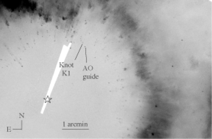
Figure 1: The location of the cometary knot K1 is plotted on the F658N ([NII]+H$\alpha$) image (O’Dell et al., 2004), together with the AO guide star. The star symbol indicates the place of the central star.

3 Description of the data

3.1 Morphology

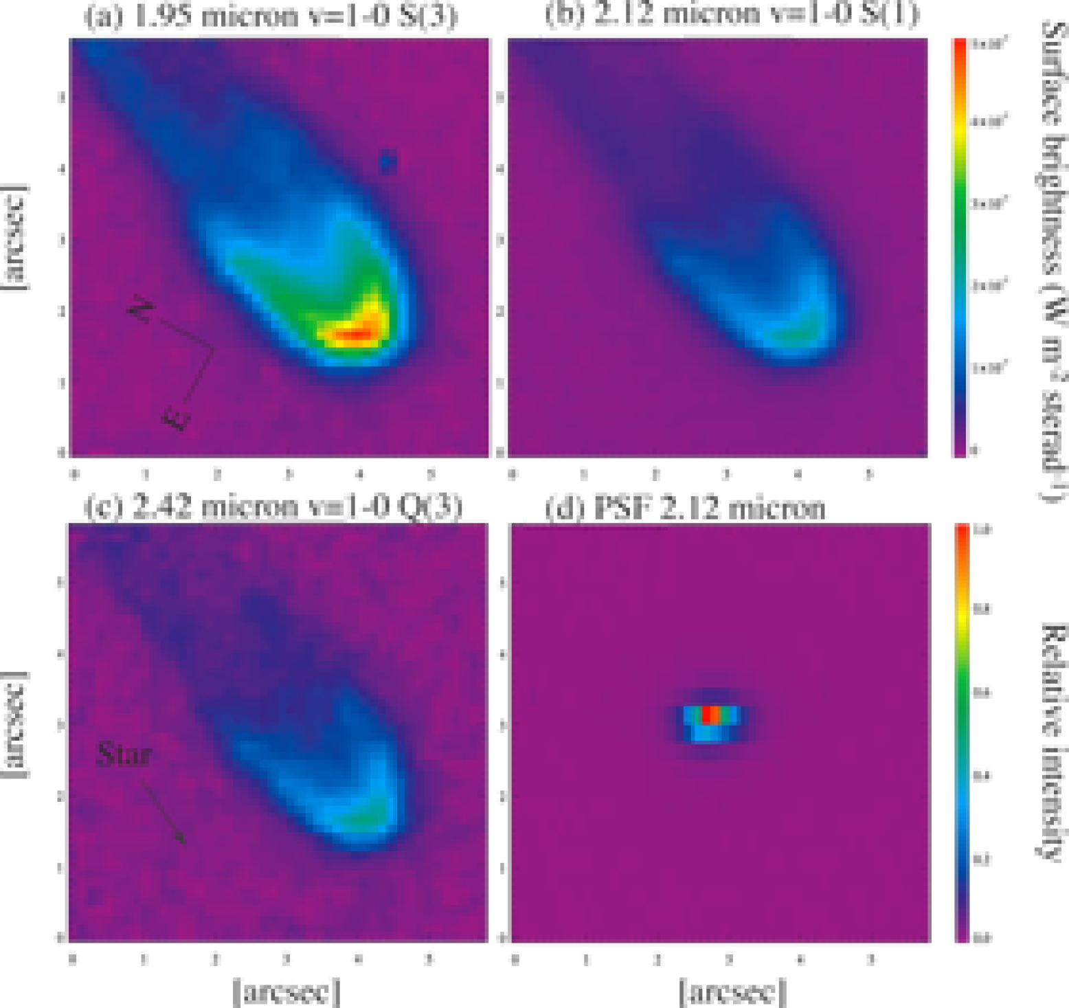
Figure 2: Images of the cometary knot K1, taken by 250 mas camera. The PSF at 2.12 $\mu$m is found in (d). The direction of the central star is marked in (c)

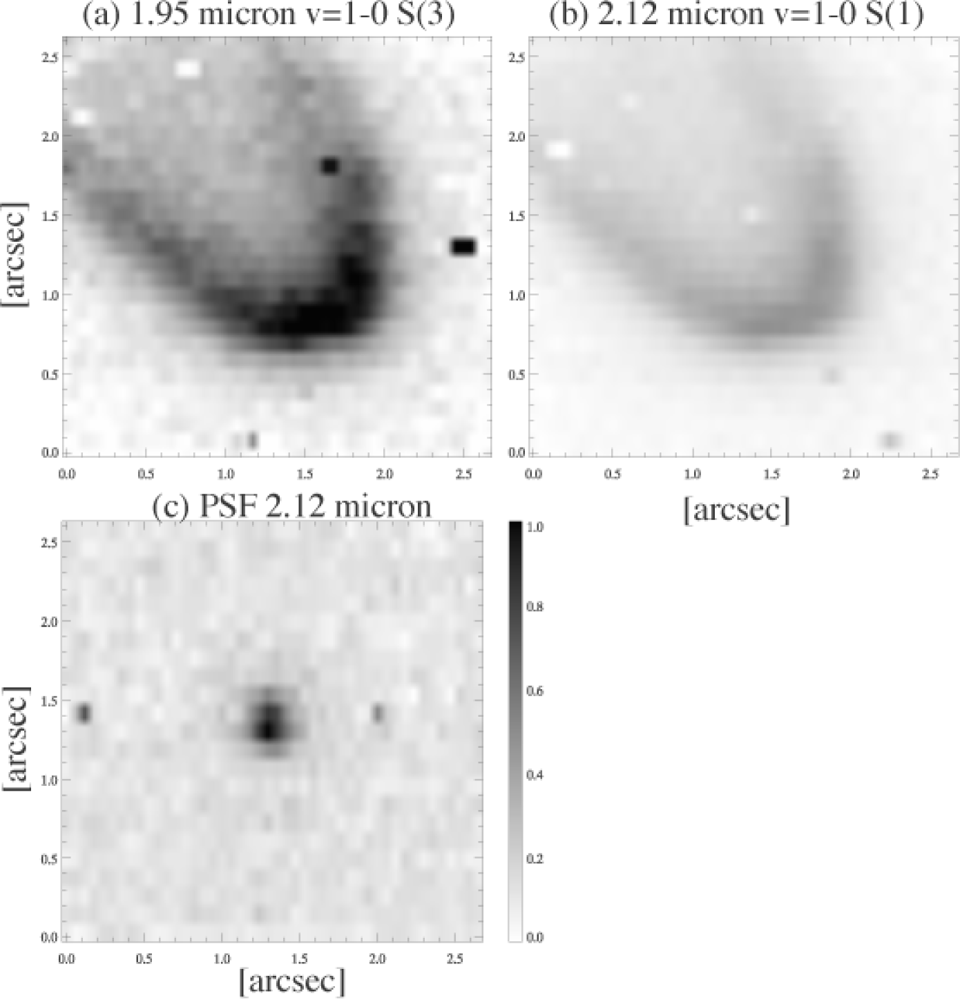
Figure 3: Image of the cometary knot K1, taken with the 100 mas camera. The PSF at 2.12 $\mu$m is found in (c).

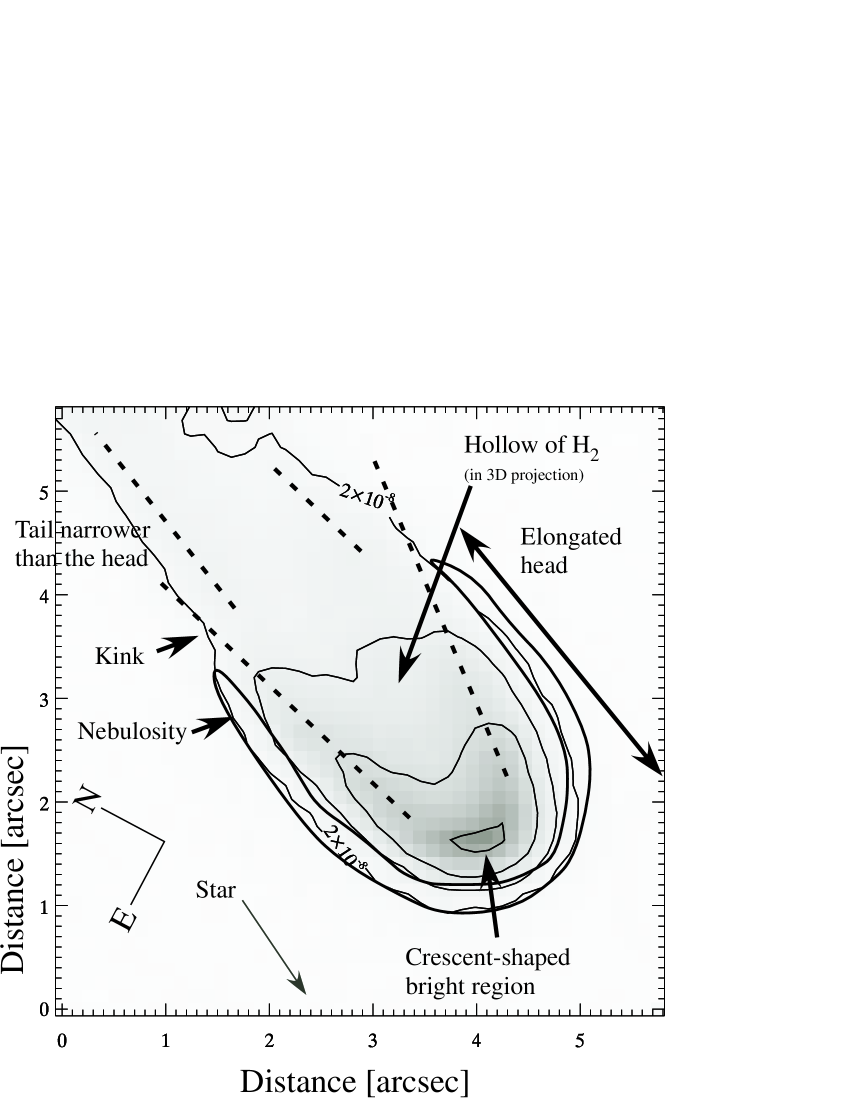
Figure 4: Annotated 2.12 $\mu$m image of the knot K1 (see text for details).

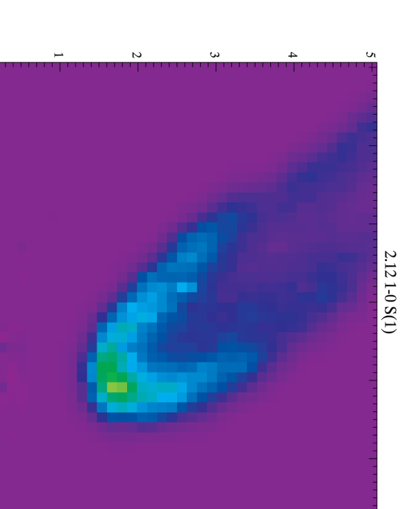
Figure 5: Deconvolved image at 2.12 $\mu$m. A fain emitting region at the rim near the crescent is found, as well as narrowing of the tail.

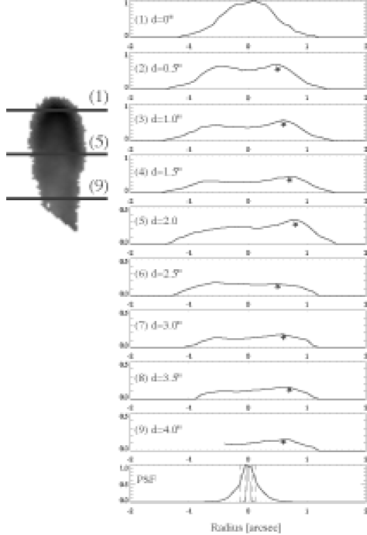
Figure 6: Cross cut of Fig. 2 along the radial axis, whose intensity is scaled to the maximum intensity of the knot. Approximate locations of cuts are indicated on the left panel. The data are smoothed with 250 mas bin along long axis of the knot. The intensity peaks on east side (right side in this figure) of the knot are marked with stars in each panel. The bottom panel shows the cross cut of the telluric standard (bold line), airy disk for 8.2 meter circular aperture (thin solid line), and pixel size (125 and 250 mas; thin dash lines). The spatial resolution is determined by the pixel scale (sampling rate). The star marks traces that the head is widen until at distance ($d$)=2.0 arcsec and then narrowing follows $d>$2.5. Tail of the PSF is less than 10 % of the peak at 0.5 arcsec.

Fig. 2 shows the image of the cometary knot K1 as seen in the three strongest H₂ lines. The knot shows an elongated head with a narrower tail. The brightest emission is found in a crescent near the tip of the head. The crescent ends in two linear segments, indicated by the dotted lines in Fig. 4 on the 2.12 $\mu$m v=1–0 S(1) image. These segments are not co-aligned and deviate from the direction of the narrower tail. Overall, this gives the impression of a ‘tadpole’ shape, as opposed to the cylindrical shape favoured by O’Dell & Handron (1996), although in either case the overall shape is largely axisymmetric. Both the linear segments and the tail are brighter on the eastern side of the knot.

The peak emission is located slightly behind the tip (Fig. 4). There is a faint nebulosity around the bright head. This faint nebulosity appears not to be the wing of the point spread function (PSF). The faint halo extends along the linear segments where the peak emission is much fainter. The higher resolution image (50 mas per pixel) in Fig. 3 also shows this faint nebulosity, suggesting that at least part of this faint nebulosity is real.

The apparent diameter at the head is about 2.5 arcsec including the faint rim, while the diameter decreases to about 2 arcsec along the tail. The transition from the linear segment to the narrower tail is visible as a kink, 2.8 arcsec from the head on east side. It is less clearly visible on the west side.

3.1.1 H₂ emission from the surface of knots

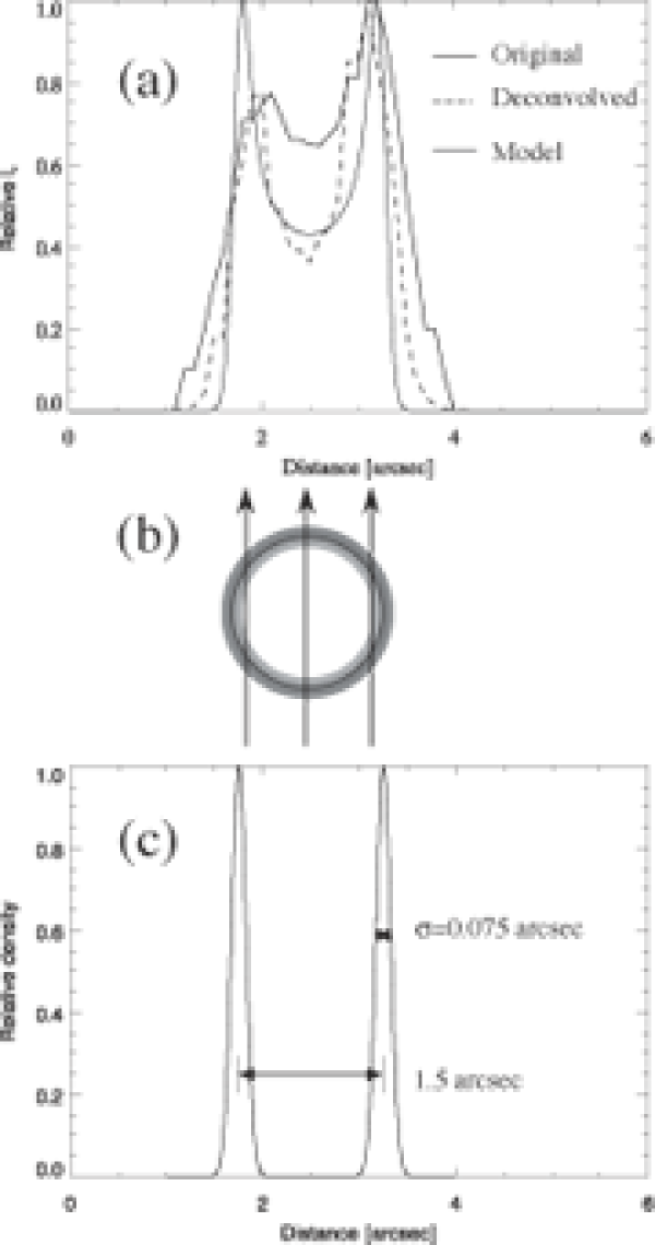
Figure 7: (a) Cross cut of the observed intensity and at 2.12 $\mu$m and PSF deconvolved profile along the radial direction in the head. The intensities are normalised at the peak. The location is 1 arcsec away from the brightest tip. Model profile in panel (a) is to demonstrate hollow shape in projected image if the knot is seen from the central star (panel b) with input parameters of the shape (panel c)

The deconvolved image (Fig. 5) shows a limb-brightened head of the knot. Within the head there may be an H₂ empty region. Fig.7 shows the radial cross-section of the head 1 arcsec inside from the brightest point. The intensity at the mid-point is about 65% of the peak in the raw image and about 40% in the deconvolved image. To demonstrate the shape, we modelled the radial profile in two dimensions, assuming a thin ring with a large hollow area inside (Fig.7 b and c). The diameter of the circular ring is 1.5 arcsec. The density structure of the ring is assumed to be a Gaussian with a width of 0.075 arcsec. The radial cut in the deconvolved image is reasonably well reproduced by this model (Fig. 7 top). The H₂ emitting region is probably a very thin surface of the knot, except at the tip.

3.1.2 Comparisons with HST [NII] and [OIII] images

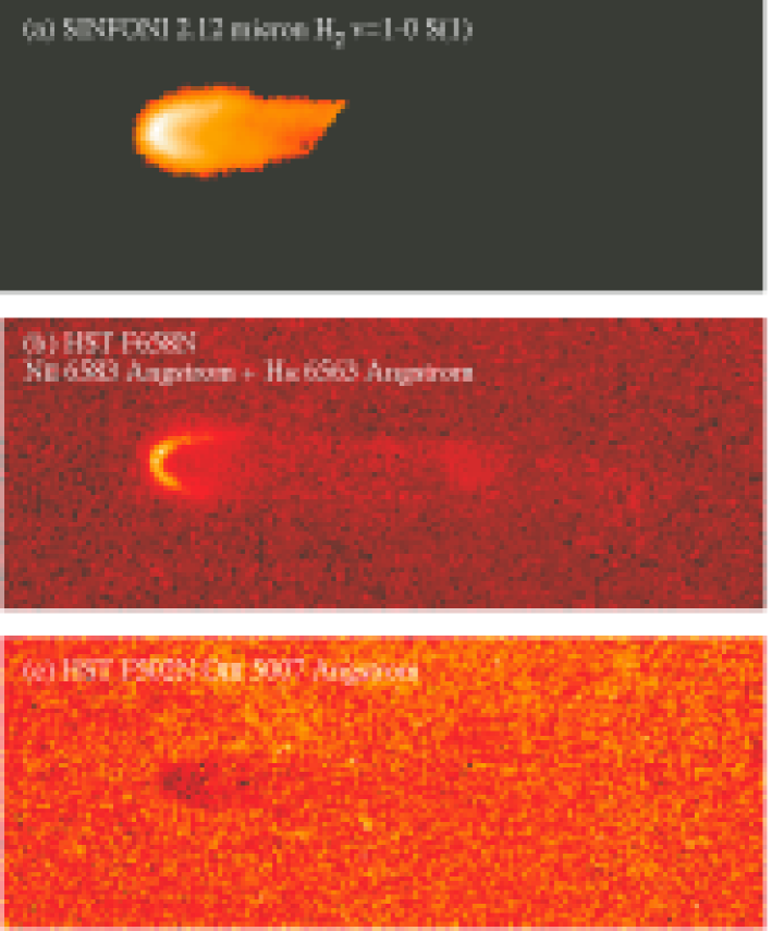
Figure 8: Comparison of the SINFONI 2.12 $\mu$m image and HST images. The SINFONI and HST images were aligned on the tip of the knot. Log intensity scale is used for all of the images. The size of the image is $22.3\times 8.5$ arcsec²

Figure 9: Cross cut of Fig. 8 along the long axis.

Fig. 8 shows the image of the knot K1 at 2.12 $\mu$m H₂ v=1–0 S(1), with a comparison of HST F658N (mainly [NII] and some contribution of H$\alpha$) and F502N ([OIII]) images from O’Dell et al. (2004). The precise alignment between SINFONI and HST images is unknown, and the images were registered such that the tip of the knot is located at the same place at [NII] and H₂ v=1–0 S(1).

The [OIII] image shows the knot in absorption; the tip is slightly off the peak from [NII] image (Fig. 9). This has also been found by O’Dell & Henney (2000) for other knots.

A cross section of the H₂ v=1–0 S(1) and [NII]+ H$\alpha$ images shows that the decay of the intensities towards the tail is very fast (almost immediate) for the ionized lines, and slower for the H₂ v=1–0 S(1). The main ionised region is a thin layer at the tip; the majority of the material remains molecular or neutral.

3.2 Spectra

Figure 10: Spectra within the knot K1 at twelve 0.675$\times$0.5 arcsec² areas defined in Fig. 11. The y-axis shows the spectral intensity from $-0.5\times 10^{8}$ to $6\times 10^{8}$ Jy sr^-1. The identifications of the H₂ transitions are indicated in panel (a).

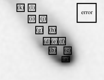
Figure 11: The twelve regions shown by boxes on the 2.12 $\mu$m image. The spectra are averaged within that area, which corresponds to the diagram in Fig. 12. The right top box is the area used to estimate the error of the intensities.

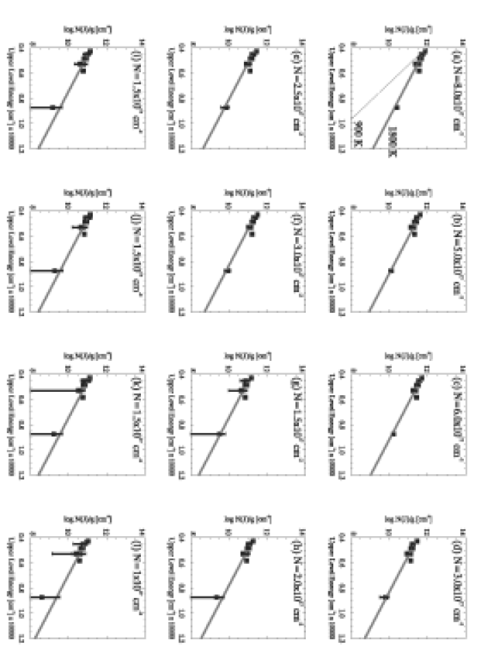
Figure 12: The energy diagrams for area (a)–(l) defined in Fig.  11; the column density for a given J upper level divided by the statistical weight as a function of upper state energy in cm^-1. The square shows the measured energy levels. The thick lines show the LTE case for 1800 K and for column densities as given in the diagrams. For a comparison, we plot the 900 K LTE line, as derived for knots in the outer region of the nebula (Cox et al., 1998) in (a). The column density for the 900 K line is $8\times 10^{18}$cm^-2. This temperature cannot fit the H₂ line intensities measured in the knot K1.

Fig. 10 shows the spectra of the knot K1 at twelve regions indicated in Fig. 11. Within each region of 5 by 5 pixels (except region (a) which has 5 by 4 pixels), the SINFONI data have been averaged. At most twelve H₂ lines (three of them with low signal-to-noise ratio) are detected by SINFONI. The intensities are summarised later in Table 2. The strongest detected line is the 1.95 $\mu$m H₂ v=1–0 S(3), and the 2.12 $\mu$m H₂ v=1–0 S(1) and 2.4 $\mu$m v=1–0 Q-branches are also strong. The H₂ lines are unresolved at the resolution of R=5090. The 2.07 $\mu$m v=2–1 S(3) and 2.15 $\mu$m v=2–1 S(2) 2.20 $\mu$m v=3-2 S(3) lines are only marginally detected.

Several high transition lines within this wavelength range are not detected, such as the 2.00 $\mu$m v=2–1 S(4), 2.38 $\mu$m v=3–2 S(1). The Br$\gamma$ line is not detected.

Table 2: Intensities of H₂ lines at area (a)–(c) and ratios with respect to the v=2–1 S(1) line.

Wav	Transition	Upper state energy		Statistical weight	Intensity $I_{\nu}$$\times 10^{7}$			Err§	Obs ratio¶
					(a)	(b)	(c)		(a)	(b)	(c)
$\mu$m		K	cm-1		W m-2sr-1
1.958	v=1–0 S(3)†	8365	5813	33	4.10	2.35	2.96	0.10	220	226	223
2.004	v=2–1 S(4)	14764	10262	13	$<$0.40§
2.034	v=1–0 S(2)	7584	5271	9	0.67	0.37	0.49	0.04	36	35	36
2.073	v=2–1 S(3)	13890	9654	33	0.08‡			0.09	4
2.128	v=1–0 S(1)	6956	4834	21	1.86	1.04	1.32	0.07	100	100	100
2.154	v=2–1 S(2)	13150	9139	9	0.07‡			0.08	3
2.201	v=3–2 S(3)	19086	13265	33	0.02‡			0.03
2.224	v=1–0 S(0)	6471	4497	5	0.42	0.24	0.31	0.06	22	23	23
2.248	v=2–1 S(1)	12550	8722	21	0.18	0.09	0.12	0.04	9	9	9
2.386	v=3–2 S(1)	17818	12384	21	$<$0.09§
2.407	v=1–0 Q(1)†	6149	4273	9	1.84	1.06	1.30	0.23	99	102	97
2.413	v=1–0 Q(2)†	6471	4497	5	0.55	0.29	0.39	0.12	29	28	29
2.424	v=1–0 Q(3)†	6956	4834	21	1.85	1.03	1.27	0.14	99	99	96
2.438	v=1–0 Q(4)†	7586	5272	9	0.57	0.31	0.38	0.18	30	30	28

^¶ Line ratio with respect to 2.128 $\mu$m v=1–0 S(1) line
^§3$\sigma$ of the noise level of the intensity in the error region indicated in Fig. 11.
^†These lines have a large ($\sim$30%) error in relative intensity calibration due to the influence of H₂O in the terrestrial atmosphere. They are excluded from the comparison with models.
^‡ Marginal detections

3.2.1 Energy diagram

Fig.  12 shows the energy diagram of the H₂ lines for several regions in the knot indicated in Fig.  11. Einstein coefficients from Turner et al. (1977) are used. The slopes in the diagrams show that the line intensities follow a $T=1800~{}$K Local Thermodynamic Equilibrium (LTE) distribution. At the bright area (a–c), the observed line intensities follow the 1800 K LTE line up to the upper energy of 8000 cm^-1. The systematic uncertainty in the absolute H₂ intensity (up to 50 per cent) affects the column density, but not the excitation temperature which is determined by the slope.

3.3 Line ratio map

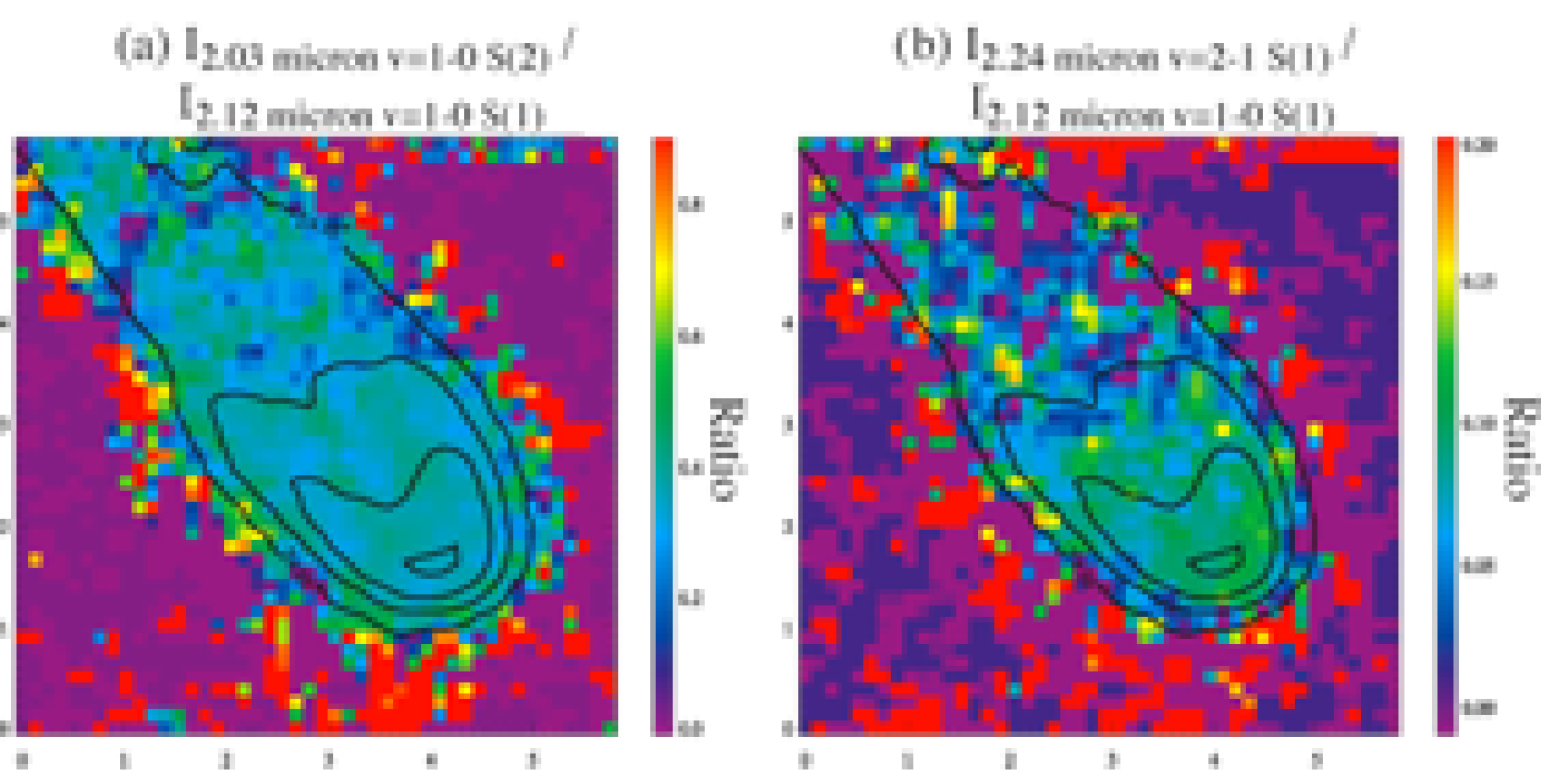
Figure 13: The line ratio maps of the cometary knot K1. The contour shows the surface brightness of 2.12 $\mu$m H₂ v=1–0 S(1) line at $0.2\times 10^{-7}$, $0.5\times 10^{-7}$, $1\times 10^{-7}$, $2\times 10^{-7}$ W m^-2 sr^-1.

Fig.  13 shows the line ratio maps within the knot. Fig.  13 (a) maps the rotational temperature variations within the knot, represented by the 2.03 $\mu$m v=1–0 S(2) and 2.12 $\mu$m v=1–0 S(1) lines. This rotational temperature is uniform within the errors throughout the knot. This uniform rotational temperature is expected from the energy diagram (Fig.  12), because all of the line intensities follow 1800 K LTE in any area.

The vibrational temperature seems to vary within the knot but this is within the uncertainty. Fig.  13 (b) shows the line ratio of 2.24 $\mu$m H₂ v=2–1 S(1) and 2.12 $\mu$m H₂ v=1–0 S(1). This is the only combination to obtain the vibrational temperature within our observed data. The line ratio tends to be highest at the tip ($\sim 0.1$) and to decrease towards the tail, although a careful treatment of v=1–0 S(0) line is needed.

4 Discussion

4.1 Excitation diagrams and temperatures

The H₂ excitation diagrams are fitted by a single LTE temperature of 1800 K. This is much higher than Cox et al. (1998) who obtained 900 K by fitting pure-rotational lines up to the S(7) transition. The region observed by Cox et al. (1998) is located at the western rim of the nebula, and is 5–6 arcmin away from the central star. The pixel size of their ISOCAM data was 6 arcsec and emission from multiple knots contributed to each single pixel. In contrast, our target is a single, isolated knot located at the innermost region of the flock of knots (2.5 arcmin from the central star).

O’Dell et al. (2007) also obtained an excitation temperature of 988 K from 5–15 $\mu$m spectra in the outer part of the nebula. O’Dell et al. (2007) state that the distance of that slit positions is similar to that of Cox et al. (1998). Although they do not provide detailed information on the slit positions and observing mode for their two Spitzer spectra, the Spitzer archive can provide this, suggesting their two slit positions are 5.6 and 4.2 arcmin from the central star, and the slit size is 3.6$\times$57 arcsec². Further three spectra at different slit positions are available in archive, but these do not fit the description of the data in O’Dell et al. (2007).

The difference in measured temperatures indicates that the excitation temperature of H₂ is not uniform within the Helix nebula: the H₂ molecules reach higher temperature within the inner region. From about 2.5 arcmin to 5 arcmin away from the central star, the excitation temperature decreases from 1800 K to 900–1000 K. This provides evidence for temperature variations within the nebula.

Hora et al. (2006) show that the [3.6]$-$[4.5] vs [4.5]$-$[8.0] colour varies within the nebula. All three bands are dominated by H₂ lines. Knots located at the inner rim of the main nebula are brighter in the 4.5 $\mu$m band. The strongest expected line in this band is the 4.69 $\mu$m H₂ 0–0 S(9), whose upper energy is the highest among the dominant H₂ lines within the IRAC filters. The colour-colour diagram of Hora et al. (2006) also suggests a higher excitation temperature in the inner region, and global variation in the excitation temperature in the entire nebula. Analysis of spectra with several slit positions within a nebula shows that the H₂ temperature is not uniform within a PN (Hora et al., 1999; Davis et al., 2003). Excitation temperature variations appear normal within a single PN.

Furthermore, H2 excitation temperatures in PNe have been found as high as 2000 K (Hora et al. 1999; Davis et al. 2003) and lower than 1000K (Cox et al., 1998; Bernard-Salas & Tielens, 2005; Matsuura & Zijlstra, 2005a). Variations in excitation temperature both between PNe and within a single PN appear to be normal

4.2 Column density

The H₂ line intensities are fitted using column densities in the range $1\times 10^{17}$–$8\times 10^{17}$ cm^-2. This range is smaller than the Cox et al. (1998) measurements of $3\times 10^{18}$ cm^-2. Our target is an isolated knot, while the low spatial resolution of the ISOCAM data almost included multiple knots within the field of view, hence the H₂ intensity is much higher (Speck et al., 2002).

The column density of H₂ can be converted to a hydrogen mass of $2\times 10^{-8}M_{\odot}$. Here we assume the knot has a column density of $4\times 10^{17}$ cm^-2 (i.e. to emit average intensity over 2$\times$2 arcsec² at the excitation temperature of 1800 K), the distance is 219 pc, the dimension of the knot is 2$\times$2 arcsec² and the density is uniform within this area. The estimated hydrogen mass is a factor of 1000 less than the estimate of O’Dell & Handron (1996), who used the extinction of the [OII] line as a mass tracer. Our infrared H₂ lines trace only highly excited H₂, as expected from the upper state energy ($>$6000 K). Colder H₂ gas is inefficient at emitting these lines (Cox et al., 1998).

In order to measure the mass of cold H₂ gas more directly, we need observations at UV wavelengths, where H₂ lines could be found in absorption. However, this approach may be compromised by the contribution to H₂ absorption by the ISM Adopting the hydrogen mass of O’Dell & Handron (1996) with a comparison of our estimated H₂ mass indicates that H₂ is heated only at the surface, but is in fact present throughout the knot. This favours a scenario where the detected H₂ was already present within the knot, i.e., it is not necessary to assume that it formed from chemical reactions from atomic/neutral hydrogen within this surface. However, this argument is based on an expected correlation between dust extinction and H₂. A direct detection is required to confirm the presence of a large, cold H₂ reservoir.

4.3 Excitation mechanisms of molecular hydrogen

The cometary knot K1 emits a 1–0 S(1) line intensity of $2\times 10^{-7}$ W m^-2 sterad^-1. The adopted uncertainty is a factor of two. The 2–1/1–0 S(1) line ratio is $\sim 0.1\pm 0.02$ at the tip, using the uncertainty on the response correction.

Burton et al. (1992) calculated the line intensities of 1–0 S(1) and 2–1 S(1) lines for J-type shocks, C-type shocks and in PDR. We found that within their model the measured line intensities and ratios can be fit equally well under several model conditions.

• A photo-dissociation region (PDR) heated by UV radiation where the density is $n=10^{6}$ cm^-3 and the UV strength is $G_{0}=1.2\times 10^{4}$ (within the range of $G_{0}=$1–1.2$\times 10^{4}$)

• C-type shocks with upstream density $n_{0}=10^{4}$ cm^-3 and shock velocity $v_{s}\sim 27$ km s^-1 (within the range of 27–28 km s^-1).

• J-type shocks $n_{0}=10^{6}$ cm^-3 and shock velocity $v_{s}\sim 9$ km s^-1(9–10 km s^-1).

Although there is some uncertainty in absolute intensity, the line ratio is the strongest constraint on the above conditions.

Meaburn et al. (1998) estimated the molecular hydrogen density of another knot to be $8.9\times 10^{5}$ cm^-3 using the extinction in the [OIII] 5007 Å  line. This knot appears brighter than K1, and larger in radius when observed in the [NII] line. We follow their method to estimate the density of the knot K1. The absorption at [OIII] is 0.73 with respect to the continuum (Sect.3.1.2). This corresponds to an extinction coefficient $c=0.15$, $E(B-V)=$0.14 mag, and an H₂ column density of $4.0\times 10^{20}$ cm^-2. If the diameter of the knot is 1.5  arcsec, an H₂ number density of $8\times 10^{4}$ cm^-3 is obtained for a distance of 219 pc. The derived H₂ density is consistent for PDR model of H₂ excitation in Burton et al. (1992).

The FUV (6–13.6 eV) flux at the knot K1 is about $G_{0}=8$, where $G_{0}$ is the FUV radiation measured in units of the Habing (1968) flux. This is based on Su et al. (2007)’s estimate assuming a luminosity of the central star of 76 $L_{\sun}$ and a distance of 219 pc. The required UV radiation in Burton et al. (1992)’s model is $G_{0}>1\times 10^{4}$, which is an order of magnitude higher than the estimated UV radiation field strength at the knot K1. We used the UCL-PDR model (Bell et al., 2005) to calculate the conditions independently. At an UV radiation field of $G_{0}=8$, we obtain a temperature below 100 K. Röllig et al. (2007) compare benchmark calculations of independent PDR codes, including the UCL-PDR model and Tielens & Hollenbach (1985)’s model that was incorporated in Burton et al. (1992)’s H₂ model. They find consistent gas temperatures among PDR models in their benchmark calculations. These results suggest that the PDR models can reproduce the measured LTE gas temperature (1800 K) of the H₂ lines in the knot K1 only, if the UV radiation strength is increased. A similar conclusion is derived by Cox et al. (1997) and O’Dell et al. (2005). The value for $G_{0}$ is defined as the flux between 6–13.6 Å  a narrow-band UV radiation field, adopted for interstellar radiation field. If we consider the continuous stellar spectrum of the central star, the UV flux increases by a factor of 10 (O’Dell et al., 2007). However, this remains a factor of 250 short of the required flux.

The speed of ambient gas for C-type shocks is $v_{s}\sim 27$ km s^-1 to fit the H₂ line intensities and line ratios, from theoretical work by Burton et al. (1992). The required velocity can vary by $\sim\pm 10$ km s^-1 depending on the assumed magnetic field strength and the iron fraction. The [HeII] and [OIII] lines show an expansion velocity of $13$ km s^-1 near the central star (Meaburn et al., 2005). Within an expanding nebula, hydrodynamic effects will cause significant velocity gradients (Schoenberner et al., 2005), as are observed in PNe (Gesicki et al., 2003). The overpressure of the ionised region dominates, and (if present) the pressure from the inner, hot bubble might be added. The same processes will occur for each knot at the ionized, facing edge. Meaburn et al. (1998, 2005) postulate turbulent velocities $\geq 10$ km s^-1 (i.e. larger than the sound speed). A C-type shock velocity could be associated with such motion. The gas density of PNe is typically $n_{0}\sim 10^{4}$ cm^-3. This is consistent with the required upstream density. C-type shock excitation of H₂ is possible. Stronger observational constraints on the velocity structure of the knot would be helpful.

The presence of magnetic fields has been reported in several young or pre-planetary nebulae using sub-mm polarization (Sabin et al., 2007). They find a magnetic field of $\sim$1mG at $5\times 10^{16}\,$cm from the central star in other PNe. The Helix knots are located 10 times further from the star than their measured location. A dipole field would decay as $r^{-3}$: this would leave a negligible field in the Helix. A solar-type field decays as $r^{-2}$, and a frozen toroidal field (as favoured by Sabin et al., 2007) may decay slower with radius. The formation of a knot may strengthen after its embedded magnetic field. The field required for the C-type shock is plausible within the knot, compared to the stronger fields detected in more compact shells. The inter-knot medium is likely to show a weaker field.

An upstream (wind) density of $10^{6}$ cm^-3 is required for the J-type shock model. Although the density within knots themselves are recorded at $10^{6}$ cm^-3 (O’Dell & Handron, 1996; Meaburn et al., 1998), it is unlikely that the upstream region has such a high density.

5 Conclusions

We have investigated the detailed structure of a single knot close to the inner edge of the main ring of the Helix nebula. We find that the rotational-vibrational temperature of H₂ is as high as 1800 K for this innermost cometary knot. The rotational temperature is uniform within the knot, and the vibrational temperature appears to follow the same distribution except for a possible decrease towards the tail. The derived temperature is much higher than previously measured (900 K) for knots in the outer region. The excitation temperature changes with radial distance from the central star. The studied knot has a wide head, with the H₂ distributed in a crescent.

We examine the possible molecular hydrogen excitation mechanisms. Based on the line intensities and ratios, C-type shocks can provide a fit using plausible local conditions, althought the required velocity is slightly higher than the observed one. This excitation requires the presence of an as-yet undetected magnetic field. A J-type shock model does not fit. We also tested the possibility that H₂ lines are excited in PDR, but PDR models have difficulties to reproduce the very high temperature, unless the UV field is increased by two orders of magnitude over the stellar radiation field. A further test of the models will require observations of the velocity structure of the head and tail. We also lack a synthesis model combining collisional and UV excitation, with hydrodynamical interactions.

6 acknowledgements

We appreciate technical support from ESO staff during the observations and the data-analysis. M.M. appreciates encouragement from Prof. Arimoto for this study. MM is grateful for hospitality at the UCL and SAAO during the visits. A discussion with Dr. M. Cohen in early stage of this research was very useful.

References

- Balick & Frank (2002) Balick B., Frank A., 2002, ARA&A 40, 439
- Beckwith et al. (1980) Beckwith S., Neugebauer G., Becklin E.E., Matthews K., Persson S.E., 1980, AJ 85, 886
- Bell et al. (2005) Bell T.A., Viti S., Williams D.A., Crawford I.A., Price R.J., 2005, MNRAS 357, 961
- Bernard-Salas & Tielens (2005) Bernard-Salas J., Tielens A.G.G.M., 2005, A&A 431, 523
- Bonnet et al. (2004) Bonnet H. et al., 2004, The ESO Messenger 117, 17
- Black & van Dishoeck (1987) Black J.H., van Dishoeck E.F., 1987, ApJ 322, 412
- Brand (2006) Brand P.W.J.L, 2006, astro-ph/0609234
- Burton et al. (1990) Burton M.G., Hollenbach D.J., Tielens A.G.G., 1990, ApJ 365, 620
- Burton et al. (1992) Burton M.G., Hollenbach D.J., Tielens A.G.G., 1992, ApJ 399, 563
- Cahn et al. (1992) Cahn J.H., Kaler J.B., Stanghellini L., 1992, A&AS 94, 399
- Cox et al. (1997) Cox P., Maillard J.-P., Huggins P.J., et al., 1997, A&A 321, 907
- Cox et al. (1998) Cox P., Boulanger F., Huggins P.J., et al., 1998, ApJ 495, L23
- Davis et al. (2003) Davis C.J., Smith M.D., Stern L., Kerr T.H., Chiar J.E., 2003, MNRAS 344, 262
- Dyson (2003) Dyson J.E., 2003, Ap&SS 285, 709
- Dyson et al. (1989) Dyson J.E., Hartquist T.W., Pettini M., Smith L.J., 1989, MNRAS 241, 625
- Dyson et al. (2006) Dyson J.E., Pittard J.M., Meaburn J., Falle S.A.E.G., 2006, A&A 457, 561
- Eisenhauer et al. (2003) Eisenhauer F., Abuter R., Bickert K., et al. 2003, SPIE 4841, 1548
- Ercolano et al. (2003) Ercolano B, Barlow M.J., Storey P.J., Liu X.-W., Rauch T., Werner K., 2003, MNRAS 344, 1145
- García-Segura et al. (2006) García-Segura G., López J. A., Steffen W., Meaburn J., & Manchado A. 2006, ApJ, 646, L61
- Gesicki et al. (2003) Gesicki K., Acker A., Zijlstra A.A., 2003, A&A, 400, 957
- Habing (1968) Habing H.J., 1968, Bull. Astr. Inst. Netherlands, 19, 421
- Harris et al. (2007) Harris H. C., et al. 2007, AJ, 133, 631
- Hora et al. (1999) Hora J.L., Latter W.B., Deutsch L.K., 1999, ApJS 124, 195
- Hora et al. (2006) Hora J.L., Latter W.B., Smith H.A., Marengo M., 2006, ApJ 652, 426
- Hollenbach & McKee (1989) Hollenbach D., McKee C.F., 1989, ApJ 342, 306
- Hollenbach & Natta (1995) Hollenbach D., Natta A., 1995, ApJ 455, 133
- Huggins et al. (2002) Huggins P.J., Forveille T., Bachiller R., Cox P., Ageorges N., Walsh J.R., 2002, ApJ 573, L55
- Huggins et al. (2005) Huggins P.J., Manley S.P., 2005, PASP 117, 665
- Kaufman & Neufeld (1996) Kaufman M.J., Neufeld D.A., 1996, ApJ 456, 611 Leahy, D. A.; Zhang, C. Y.; Kwok, Sun 1994, ApJ 422, 205
- Likkel et al. (2006) Likkel L., Dinerstein H.L., Lester D.F. Kindt A., Bartig K., 2006, AJ 131, 1515
- Matsuura & Zijlstra (2005a) Matsuura M., Zijlstra A.A., 2005a, High Resolution Infrared Spectroscopy in Astronomy, Edited by H.U. Käufl, R. Siebenmorgen, and A.F.M. Moorwood, Springer-Verlag, Berlin/Heidelberg, p. 423
- Matsuura et al. (2005b) Matsuura M., Zijlstra A.A., Molster F.J., Waters L.B.F.M., Nomura H., Sahai R., Hoare M.G., 2005b, MNRAS 359, 383
- McCaughrean & Mac Low (1997) McCaughrean M.J., Mac Low M.-M., 1997, AJ 113, 391
- Meaburn et al. (1998) Meaburn J., Clayton C.A., Bryce M., Walsh J.R., Holloway A.J., Steffen W., 1998, MNRAS 294, 201
- Meaburn et al. (2005) Meaburn J., Boumis P., López, J.A., Harman D.J., Bryce M., Redman M.P., Mavromatakis F., 2005, MNRAS 360, 963
- Meixner et al. (2005) Meixner M., McCullough P., Hartman J., Son M., Speck A., 2005, AJ 130, 1784
- Modigliani et al. (2007) Modigliani A., Hummel W., Amico P., et al., 2007 Proceedings ADA IV (astro-ph/0701297)
- Natta & Hollenbach (1998) Natta A., Hollenbach D., 1998, A&A 337, 517
- Neufeld & Dalgarno (1989) Neufeld D.A., Dalgarno A., 1989, ApJ 340, 869
- O’Dell & Handron (1996) O’Dell C.R., Handron K.D., 1996, AJ 111, 1630
- O’Dell & Henney (2000) O’Dell C.R., Henney W.J., Burkert A., 2000, AJ 119, 2910
- O’Dell et al. (2002) O’Dell, C. R., Balick, B., Hajian, A. R., Henney, W. J., & Burkert, A. 2002, AJ, 123, 3329
- O’Dell et al. (2005) O’Dell C.R., Henney W.J., Ferland G.J., 2005, AJ 130, 172
- O’Dell et al. (2007) O’Dell C.R., Henney W.J., Ferland G.J., 2007, AJ, in press (astro-ph/0701636)
- O’Dell et al. (2004) O’Dell C.R., McCullough P.R., Meixner M., 2004, AJ 128, 2339
- Pickles (1998) Pickles A.J., 1998, PASP 110, 863
- Pittard et al. (2005) Pittard J.M., Dyson J.E., Falle S.A.E.G., Hartquist T.W., 2005, MNRAS 361, 1077
- Redman et al. (2003) Redman M.P., Viti S., Cau P., Williams D.A., 2003, MNRAS 345, 1291
- Röllig et al. (2007) Röllig M., Abel N.P., Bell T., et al., 2007 A&A in press (astro-ph/0702231)
- Sabin et al. (2007) Sabin L., Zijlstra A.A., Greaves J.A., 2007, MNRAS in press (astro-ph/070154)
- Schoenberner et al. (2005) Schoenberner D., Jacob R., Steffen M. 2005, A&A 441, 573
- Speck et al. (2002) Speck A.K., Meixner M., Fong D., McCullough P.R., Moser D.E., Ueta T., 2002, AJ 123, 346
- Speck et al. (2003) Speck A.K., Meixner M., Jacoby G.H., Knezek P.M., 2003, PASP 115, 170
- Su et al. (2007) Su K.Y.L., Chu Y.-H., Rieke G.H., et al., 2007 2007, ApJ 657, L41
- Tielens & Hollenbach (1985) Tielens A.G.G.M., Hollenbach D., 1985, ApJ 291, 747
- Turner et al. (1977) Turner J., Kirby-Docken K., Dalgarno A., 1977, ApJS 35, 281
- Vishniac (1994) Vishniac E.T., 1994, ApJ 428, 186
- Woods (2004) Woods P.M., 2004, PhD Thesis, UMIST, UK
- Zuckerman & Gatley (1988) Zuckerman B., Gatley I., 1988, ApJ 324, 501