Splitting of Andreev levels in a Josephson junction by spin-orbit coupling

Abstract

We consider the effect of spin-orbit coupling on the energy levels of a single-channel Josephson junction below the superconducting gap. We investigate quantitatively the level splitting arising from the combined effect of spin-orbit coupling and the time-reversal symmetry breaking by the phase difference between the superconductors. Using the scattering matrix approach we establish a simple connection between the quantum mechanical time delay matrix and the effective Hamiltonian for the level splitting. As an application we calculate the distribution of level splittings for an ensemble of chaotic Josephson junctions. The distribution falls off as a power law for large splittings, unlike the exponentially decaying splitting distribution given by the Wigner surmise – which applies for normal chaotic quantum dots with spin-orbit coupling in the case that the time-reversal symmetry breaking is due to a magnetic field.

I Introduction

A Josephson junction is a weak link between two superconductors with an adjustable phase difference $\phi$. The weak link may be a tunnel barrier or a normal metal. Fig. 1 shows, for example, a Josephson junction consisting of a small piece of normal metal (a quantum dot), connected to the superconductors by a pair of narrow constrictions (quantum point contacts). The excitation spectrum below the superconducting gap $\Delta$ consists of discrete energies, called Andreev levels. In zero magnetic field, the energy levels $\varepsilon_{n}$ are determined by the normal-state transmission eigenvalues $T_{n}$ if $\Delta\ll\hbar/\tau_{\rm dw}$, where $\tau_{\rm dw}$ is the dwell time of an electron in the normal region (before it is converted into a hole by Andreev reflection at the superconductor). The relationship isBeenakker (1991)

$$\varepsilon_{n}=\Delta\sqrt{1-T_{n}\sin^{2}(\phi/2)}+{\cal O}(\Delta^{2}\tau_{\rm dw}/\hbar).$$ (1)

Each level is twofold spin-degenerate (Andreev doublet).

Recently the effect of spin-orbit coupling on Josephson junctions became a subject of investigationBezuglyi et al. (2002); Chtchelkatchev and Nazarov (2003); Krive et al. (2004); Dimitrova and Feigel’man (2006); Dell’Anna et al. (2007). This is a subtle effect for the following reason: On the one hand, in the absence of magnetic fields the normal-state transmission eigenvalues $T_{n}$ are Kramers degenerate because of the time-reversal invariance of the normal system. On the other hand, one would expect a breaking of the degeneracy of the Andreev doublets because the phase difference between the superconducting contacts breaks the time-reversal symmetry of the system. Still, to leading order in $\Delta\tau_{\rm dw}/\hbar$ the one-to-one relationship (1) between $\varepsilon_{n}$ and $T_{n}$ ensures that the Andreev levels remain degenerate for nonzero $\phi$. As was pointed out by Chtchelkatchev and NazarovChtchelkatchev and Nazarov (2003), to see a splitting of the Andreev doublets as a result of the combined effect of spin-rotation symmetry breaking by spin-orbit coupling and time-reversal symmetry breaking by the phase difference one has to go beyond the leading order in $\Delta\tau_{\rm dw}/\hbar$. This tunable level splitting was exploited in a proposal of Andreev qubits for quantum computationChtchelkatchev and Nazarov (2003).

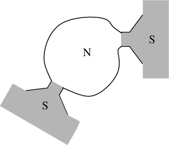
Figure 1: Sketch of a quantum dot Josephson junction: the quantum dot (N) is connected to two superconductors (S) by point contacts. Spin-orbit coupling splits the energy levels of the system when the superconductors have a nonzero phase difference.

In this work we examine the splitting of the Andreev doublets quantitatively by calculating the first order correction to the energy levels in the small parameter $\Delta\tau_{\rm dw}/\hbar$. We concentrate our attention on the case when the quantum point contacts support one propagating mode each. We give a simple relation between the effective Hamiltonian for the level splitting of Chtchelkatchev and NazarovChtchelkatchev and Nazarov (2003) and the Wigner-Smith time delay matrix,

$$Q=-iS^{\dagger}\frac{dS}{d\varepsilon},$$ (2)

where $S$ is the scattering matrix of the normal system. As an application, we calculate how the splittings are distributed for an ensemble of systems where the two superconductors are connected by a chaotic quantum dot, assuming that the spin-orbit coupling in the dot is strong enough that the dot Hamiltonian can be modeled as a member of the symplectic ensemble of Random Matrix Theory (RMT)Mehta (2004); Beenakker (1997). The present study in the regime $\Delta\ll\hbar/\tau_{\rm dw}$ complements earlier workAltland and Zirnbauer (1997); Béri et al. (2007) in the opposite regime $\Delta\gg\hbar/\tau_{\rm dw}$.

The paper is organized as follows. In Sec. II we employ the scattering matrix approach for calculating the first order correction in $\Delta\tau_{\rm dw}/\hbar$ to the Andreev levels, and obtain the effective Hamiltonian for the level splitting in terms of the time delay matrix $Q$. For simplicity, we consider the single-channel case in Sec. II and give the multichannel extension in an Appendix. We apply our single-channel formula to a calculation of the splitting distribution for an ensemble of chaotic Josephson junctions in Sec. III. We conclude in Sec. IV with a comparison of the splitting distribution of the Andreev doublets and the Wigner surmise of RMT.

II Splitting Hamiltonian and Wigner-Smith matrix

For energies below the superconducting gap $\Delta$ the Josephson junction supports bound states, with excitation energies given by the roots of the secular equationBeenakker (1991)

$${\rm Det}\,\left[\openone-\alpha(\varepsilon)^{2}r_{\rm A}^{\ast}S_{\rm e}(\varepsilon)r_{\rm A}S_{\rm h}(\varepsilon)\right]=0,$$ (3)

where

$$\alpha=\exp\left[-{\rm i}\arccos\left(\frac{\varepsilon}{\Delta}\right)\right],\,r_{\rm A}={\left(\begin{array}[]{cc}{\rm e}^{{\rm i}\phi/2}\openone&0\\ 0&{\rm e}^{-{\rm i}\phi/2}\openone\end{array}\right)},$$ (6)

and $S_{\rm e}(\varepsilon)$ and $S_{\rm h}(\varepsilon)$ are the scattering matrices of the normal system for electrons and holes. They are related as

$$S_{\rm h}(\varepsilon)=\mathcal{T}S_{\rm e}(-\varepsilon)\mathcal{T}^{-1},$$ (7)

where $\mathcal{T}=i\sigma_{2}K$ is the time-reversal operator for spin-$1/2$ particles. The matrix $\sigma_{2}$ is the second Pauli matrix acting on the spin degree of freedom and $K$ is the operator of complex conjugation. Relation (7) reflects the fact that in the normal part the dynamics of the holes is governed by the Hamiltoniande Gennes (1966)

$$H_{\rm h}=-\mathcal{T}H_{\rm e}\mathcal{T}^{-1},$$ (8)

the negative of the time reversed electron Hamiltonian $H_{\rm e}$.

We consider the case when the normal part is time-reversal invariant, which imposes the self duality condition $S=\sigma_{2}S^{T}\sigma_{2}$ on the scattering matrix. (The superscript $T$ refers to matrix transposition.) The elements of $S_{\rm e}(\varepsilon)$ change significantly if $\varepsilon$ is changed on the scale of $\hbar/\tau_{\rm dw}$, therefore to leading order in $\Delta\tau_{\rm dw}/\hbar$ one can neglect the energy dependence of $S_{\rm e}(\varepsilon)$, and take it at the Fermi energy, $S_{\rm e}(\varepsilon)\approx S_{\rm e}(0)$. Making use of the self-duality of the scattering matrix, and introducing the usual block structure

$$S=\left(\begin{array}[]{cc}r&t^{\prime}\\ t&r^{\prime}\end{array}\right),$$ (9)

the secular equation (3) can be simplified toBeenakker (1991)

$${\rm Det}\left[\left(1-\frac{\varepsilon^{2}}{\Delta^{2}}\right)-t^{\dagger}t\sin^{2}\left(\frac{\phi}{2}\right)\right]=0.$$ (10)

From this equation follows the relation (1) between the energies and the transmission eigenvalues.

The correction of order $\Delta^{2}\tau_{\rm dw}/\hbar$ comes from considering the energy dependence of the scattering matrix to first order, $S(\varepsilon)\approx S(0)+(dS/d\varepsilon)\varepsilon$. For simplicity, we restrict ourselves here to the case of two single-channel point contacts. (The extension to multichannel point contacts is given in App. A.) For single-channel point contacts the self-duality of the scattering matrix implies

$$r=\rho\openone_{2},\ r^{\prime}=\rho^{\prime}\openone_{2},\ t^{\prime}=\sigma_{2}t^{T}\sigma_{2},\ t=\sqrt{T}U,$$ (11)

where $\rho,\ \rho^{\prime}$ are complex numbers, $\openone_{2}$ is the $2\times 2$ unit matrix, $1\geq T\geq 0$ and $U$ is a $2\times 2$ unitary matrix. Writing the energy as $\varepsilon_{0}+\delta\varepsilon$ with

$$\varepsilon_{0}=\Delta\sqrt{1-T\sin^{2}(\phi/2)},$$ (12)

and keeping terms up to linear order in the small quantities $\delta\varepsilon={\cal O}(\Delta^{2}\tau_{\rm dw}/\hbar)$ and $\Delta\tau_{\rm dw}/\hbar$, one finds the eigenvalue equation

$${\rm Det}\left[\frac{\Delta^{2}}{4}\left(\sigma_{2}Q^{T}_{11}\sigma_{2}-Q_{11}\right)\sin(\phi)\right.\\ \left.\mbox{}-\frac{\Delta^{2}}{4}({\rm Tr}\ Q)\frac{\varepsilon_{0}}{\Delta}\sqrt{1-\frac{\varepsilon_{0}^{2}}{\Delta^{2}}}\ \openone_{2}-\delta\varepsilon\right]=0$$ (13)

for the energy correction $\delta\varepsilon$. The matrix $Q$ has the block structure

$$Q=\begin{pmatrix}Q_{11}&Q_{12}\\ Q_{21}&Q_{22}\end{pmatrix},$$ (14)

inherited from the transmission-reflection block structure (9) of the scattering matrix.

The second term in the determinant (13) shifts both eigenvalues by the same amount $\delta\varepsilon_{\rm shift}$, while the first, manifestly traceless term is responsible for the splitting $\pm\delta\varepsilon_{\rm split}$ of the doublet. We see that the splitting is determined by the effective Hamiltonian

$$H_{\rm eff}=\Delta\frac{\tau_{\rm dw}\Delta}{\hbar}\ \Sigma\ \sin(\phi),$$ (15)

with $\Sigma$ a traceless Hermitian $2\times 2$ matrix having matrix elements of order unity. This is the result of Chtchelkatchev and NazarovChtchelkatchev and Nazarov (2003). Our analysis gives an explicit relationQ11Q22 between the matrix $\Sigma$ and the time delay matrix $Q$,

$$\Sigma=\frac{\hbar}{4\tau_{\rm dw}}\left(\sigma_{2}Q^{T}_{11}\sigma_{2}-Q_{11}\right).$$ (16)

This is the key relation that will allow us, in the next section, to calculate the level splitting distribution from the known properties of the time delay matrix in a chaotic system.

Figure 2: A schematic illustration of the splitting of the Andreev doublet as a function of the phase difference $\phi$ for a single-channel Josephson junction with spin-orbit coupling. The energies are the sum of a degenerate part $\varepsilon_{0}+\delta\varepsilon_{\rm shift}$ that is even in $\phi$ and a splitting $\pm\delta\varepsilon_{\rm split}$ that is odd in $\phi$, as explained in the text. The maximal splitting is reached at $\phi=\pi/2$.

We conclude this section with a symmetry consideration. The shift $\delta\varepsilon_{\rm shift}$ is even in $\phi$, just like the zeroth order term $\varepsilon_{0}$. In contrast, the splitting $\delta\varepsilon_{\rm split}$ is odd in $\phi$. This is in accord with the symmetry of the Hamiltonian $H$ that gives the full excitation spectrum of the Josephson junction. Under time reversal, in our case of a time-reversal invariant normal part, it transforms as $\mathcal{T}H(\phi)\mathcal{T}^{-1}=H(-\phi)$, therefore, for an eigenstate $\Psi$ one has

$$\begin{array}[]{lll}H(\phi)\Psi(\phi)&=&\varepsilon(\phi)\Psi(\phi),\\ H(\phi)\mathcal{T}\Psi(-\phi)&=&\varepsilon(-\phi)\mathcal{T}\Psi(-\phi).\par\end{array}$$ (17)

An Andreev doublet is therefore of the form $\{\varepsilon(\phi),\varepsilon(-\phi)\}$. The decomposition of $\varepsilon(\phi)$ into even and odd parts in $\phi$ amounts to a decomposition of the doublet into a degenerate even part and an odd splitting part. The resulting $\phi$ dependence of the doublet is shown schematically in Fig. 2.

III Splitting distribution in chaotic Josephson junctions

As an application of our general result (16) we calculate how the level splittings are distributed for an ensemble of Josephson junctions where the normal part is a chaotic quantum dot. We assume that the spin-orbit coupling inside the dot is strong enough that the dot Hamiltonian can be modeled as a member of the symplectic ensemble of RMT, i.e. that the spin-orbit time $\tau_{\rm so}$ is much shorter than $\tau_{\rm dw}$.

The splitting distribution can be obtained from the known distribution of the scattering matrixBeenakker (1997), and of the dimensionless symmetrized Wigner-Smith matrixBrouwer et al. (1997),

$$Q_{E}=-i\ \frac{\hbar}{\tau_{\rm dw}}\,S^{-1/2}(dS/d\varepsilon)S^{-1/2}.$$ (18)

The distributions of $S$ and $Q_{E}$ are independentBrouwer et al. (1997), which makes it advantageous to express $Q$ in terms of $S$ and $Q_{E}$:

$$Q=\frac{\tau_{\rm dw}}{\hbar}S^{-1/2}Q_{E}S^{1/2}.$$ (19)

In the single-channel case one has

$$\begin{array}[]{c}Q_{E}=M_{1}\left(\begin{array}[]{cc}1/\gamma_{1}\ \openone_{2}&0\\ 0&1/\gamma_{2}\ \openone_{2}\end{array}\right)M_{1}^{\dagger},\\ \\ S=M_{2}\left(\begin{array}[]{cc}e^{i\varphi_{1}}\openone_{2}&0\\ 0&e^{i\varphi_{2}}\openone_{2}\end{array}\right)M_{2}^{\dagger}.\end{array}$$ (20)

The rates $\gamma_{n}$ are distributed according toBrouwer et al. (1997)

$$P(\gamma_{1},\gamma_{2})\propto|\gamma_{1}-\gamma_{2}|^{4}\ \gamma_{1}^{4}\gamma_{2}^{4}\ \exp[-{4(\gamma_{1}+\gamma_{2})}].$$ (21)

The distribution of the phases $\phi_{n}$ isBeenakker (1997)

$$P(\phi_{1},\phi_{2})\propto|e^{i\phi_{1}}-e^{i\phi_{2}}|^{4}.$$ (22)

The matrices of eigenvectors $M_{1}$ and $M_{2}$ are members of the group Sp(2) of $4\times 4$ unitary symplectic matrices, and are uniformly distributed with respect to the Haar measure of the groupBeenakker (1997); Brouwer et al. (1997). The Haar measure is given as

$$d\mu\propto\sqrt{|{\rm Det}g|}\Pi_{j}dx_{j},$$ (23)

in terms of the metric tensor $g$, defined by

$${\rm Tr}\left(dMdM^{\dagger}\right)=\sum_{ij}g_{ij}dx_{i}dx_{j}.$$ (24)

Here $\{x_{i}\}$ is a set of independent variables parameterizing the Sp(2) matrix $M$.

A convenient choice to parameterize Sp(2) is the decomposition

$$M=\left(\begin{array}[]{cc}\cos(\theta)&\sin(\theta)\ W\\ -\sin(\theta)\ W&\cos(\theta)\end{array}\right)\ \left(\begin{array}[]{cc}U&0\\ 0&V\end{array}\right),$$ (25)

where $W$, $U$ and $V$ are SU(2) matrices, and $\theta\in[0,\pi/2]$. It is seen that the SU(2)$\otimes$SU(2) factor corresponding to the block-diagonal matrix with $U$ and $V$ cancels from the spectral decomposition (20) of $Q_{E}$ and $S$. Using the Euler angle parameterization for SU(2),

$$\begin{array}[]{c}U\!\!=\!\!\!\!\ \left(\begin{array}[]{cc}e^{-i(\phi_{U}+\psi_{U})/2}\cos(\theta_{U}/2)&-e^{i(\psi_{U}-\phi_{U})/2}\sin(\theta_{U}/2)\\ e^{i(\phi_{U}-\psi_{U})/2}\sin(\theta_{U}/2)&e^{i(\phi_{U}+\psi_{U})/2}\cos(\theta_{U}/2)\end{array}\right)\!\!,\\ \\ \phi_{U}\in[0,2\pi],\ \psi_{U}\in[0,4\pi],\ \theta_{U}\in[0,\pi],\end{array}$$ (26)

and similarly for the matrices $V$, $W$, one finds that the Haar measure on Sp(2) corresponding to the chosen parameterization is

$$d\mu(M)\propto\sin^{3}(\theta)\cos^{3}(\theta)d\theta\!\prod_{j=U,V,W}\!\sin(\theta_{j})d\phi_{j}d\theta_{j}d\psi_{j}.$$ (27)

Figure 3: Main plot: Distribution of the maximal splitting of the Andreev levels (reached at $\phi=\pi/2$) in units of $\Delta^{2}\tau_{\rm dw}/\hbar$. The smooth curve is the prediction of Random Matrix Theory calculated from Eq. (29), the histogram is the result of a numerical simulation using the spin kicked rotator. Inset: comparison of the Andreev doublet splitting distribution (solid line) and the Wigner surmise (dashed line). For this comparison, the energies are rescaled such that the mean of the distributions is unity.

We define the maximal dimensionless splitting $q$ of the Andreev levels (reached at $\phi=\pi/2$) by the formula

$$\delta\varepsilon_{\rm split}=q\Delta\frac{\Delta\tau_{\rm dw}}{\hbar}\sin(\phi).$$ (28)

The distribution of $q$ is given by

$$\begin{array}[]{c}P(q)=\int d\mu(S)d\mu(Q_{E})\delta(q-\sqrt{-\rm{Det}(\Sigma)}),\\ \\ d\mu(Q_{E})=d\mu(M_{1})d\gamma_{1}d\gamma_{2}P(\gamma_{1},\gamma_{2}),\\ \\ d\mu(S)=d\mu(M_{2})d\varphi_{1}d\varphi_{2}P(\varphi_{1},\varphi_{2}).\\ \end{array}$$ (29)

Eq. (29) can be evaluated numerically. The resulting distribution is shown in Fig. 3. The first two moments of $q$ are

$$\langle q\rangle=0.181,\quad\sqrt{\langle q^{2}\rangle-\langle q\rangle^{2}}=0.152\ \ .$$ (30)

The splitting distribution near zero behaves as

$$P(q)\sim q^{2}\quad(q\rightarrow 0).$$ (31)

For large splittings we find

$$P(q)\sim q^{-6}\quad(q\rightarrow\infty).$$ (32)

In order to check our prediction (29) for the level splitting distribution, we have numerically simulated the chaotic quantum dot Josephson junction of Fig. 1 using the spin kicked rotatorScharf (1989); Bardarson et al. (2005). The spin kicked rotator is a dynamical model, from which one can extract scattering matrices characteristic of chaotic cavities. These scattering matrices are given by

$$S(\varepsilon)={\cal P}[e^{-i\varepsilon}-{\mathcal{F}}(1-{\cal P}^{T}{\cal P})]^{-1}{\mathcal{F}}{\cal P}^{T},$$ (33)

where $\mathcal{F}$ is a $2M\times 2M$ matrix giving the stroboscopic time evolution of the model and ${\cal P}$ is a $4\times 2M$ projection matrix projecting onto the two single-channel point contacts (the factors of $2$ in the dimensions are because of the spin). The quasienergy $\varepsilon$ plays the role of the energy variable, measured in units of $\hbar/t_{0}$ with $t_{0}$ the stroboscopic time. For a more detailed description of this numerical model we refer the reader to Ref. Bardarson et al., 2005.

Scattering matrices generated through Eq. (33) are inserted into the secular Eq. (3), and the roots are found by varying the quasienergy. The dwell time in this model is $\tau_{\rm dw}=M/2$ (again in units of $t_{0}$). We take $M=100$ and $\Delta=2\cdot 10^{-4}$ (in units of $\hbar/t_{0}$), so that $\Delta\tau_{\rm dw}/\hbar=10^{-2}\ll 1$. By sampling about $10^{5}$ different ${\cal F}$, $P$, and $\phi$ we numerically obtain the distribution $P(q)$ shown in Fig. 3 together with the analytical result (29). The agreement is very good.

IV Discussion

IV.1 Summary

We have investigated the effect of spin-orbit coupling on the subgap spectrum of single-channel Josephson junctions. Using the scattering matrix approach and considering the energy dependence of the scattering matrix to first order we obtained a simple relation, Eq. (16), between the effective Hamiltonian governing the level splitting and the quantum mechanical time delay matrix $Q=-iS^{\dagger}dS/d\varepsilon$. This relation allowed us to find the splitting distribution for an ensemble of chaotic Josephson junctions using the known properties of $Q$. We verified our result numerically by simulating the chaotic Josephson junction using the spin kicked rotator, and we found excellent agreement.

IV.2 Comparison of the splitting distribution with the Wigner surmise

In the inset of Fig. 3 we compare the splitting distribution of the Andreev doublet with the Wigner surmise of RMTMehta (2004),

$$P_{\rm W}(x)=\frac{32}{\pi^{2}}\ x^{2}\ \exp\left(-\frac{4x^{2}}{\pi}\right).$$ (34)

(For this comparison the energy scale is set such that the average splitting is unity.) The motivation behind this comparison is the fact that the Wigner surmise is also a splitting distribution: as shown in App. B it describes the distribution of the splittings of Kramers doublets for normal chaotic quantum dots with spin-orbit coupling in the case that the time-reversal symmetry is broken by a magnetic field.

At small splittings, both $P$ and $P_{\rm W}$ decay quadratically. This quadratic decay is a generic feature of the splitting of a Kramers degenerate level due to time-reversal symmetry breaking. It follows from the fact that the splitting Hamiltonian is a $2\times 2$ Hermitian traceless matrix without further symmetries and from a power counting argumentHaake (2001) similar to the one leading to the quadratic decay of $P_{\rm W}$.

While at small splittings the two distributions decay in the same way, we find qualitative differences in the opposite limit. At large splittings $P$ decays like a power law in contrast to the exponential decay of $P_{\rm W}$ [cf. Eqs. (32) and (34)].

We attribute the deviation of $P$ from the Wigner surmise to the nonuniform way in which time-reversal symmetry is broken: While the magnetic field in App. B acts uniformly throughout the normal quantum dot, the superconducting phase difference in the Josephson junction acts nonuniformly at the point contacts.

Appendix A Splitting Hamiltonian for multichannel Josephson junctions

We generalize the relation (16) between the splitting Hamiltonian and the time delay matrix to the case that each of the two point contacts supports $N/2$ propagating modes. (The single-channel case of Sec. II therefore corresponds to $N=2$.) In the multichannel case, after the steps leading to Eq. (13) one arrives at the equation

$${\rm Det}\left[H_{0}+\frac{\Delta^{2}}{2}\ K-\delta\varepsilon\right]=0,$$ (35)

where

$$H_{0}=\frac{\Delta^{2}}{2\varepsilon_{n}^{(0)}}\left[1-\left(\frac{\varepsilon_{n}^{(0)}}{\Delta}\right)^{2}-t^{\dagger}t\sin^{2}\left(\frac{\phi}{2}\right)\right],$$ (36)

$$\varepsilon_{n}^{(0)}=\Delta\sqrt{1-T_{n}\sin^{2}(\phi/2)},$$ (37)

and $K$ is a matrix with elements of order $\tau_{\rm dw}/\hbar$. An eigenvector of $t^{\dagger}t$ with eigenvalue $T_{n}$ is also an eigenvector of $H_{0}$ with zero eigenvalue. The first order correction to the zeroth order energy $\varepsilon_{n}^{(0)}$ is the first order perturbative correction to this zero eigenvalue.

We introduce the $N\times 2$ matrices $W_{n}$ and $W_{n}^{\prime}$ which contain the two orthonormal eigenvectors of, respectively, $t^{\dagger}t$ and $t^{\prime\dagger}t^{\prime}$, both corresponding to the eigenvalue $T_{n}$. In terms of these matrices we define the matrices $q_{1n}$ and $q_{2n}$ by

$$q_{1n}=W_{n}^{\dagger}Q_{11}W_{n},\quad q_{2n}=W_{n}^{\prime\dagger}Q_{22}W_{n}^{\prime}\ .$$ (38)

We find that the shift of the Andreev doublet at $\varepsilon_{n}^{(0)}$ is given by

$$\delta\varepsilon_{n}^{\rm shift}=-\frac{\Delta^{2}}{4}\frac{\varepsilon_{n}^{(0)}}{\Delta}\sqrt{1-\left(\varepsilon_{n}^{(0)}/\Delta\right)^{2}}\left({\rm Tr}\ q_{1n}+{\rm Tr}\ q_{2n}\right),$$ (39)

while the splitting $\delta\varepsilon_{n}^{\rm split}$ is given by the two eigenvalues of the traceless Hermitian matrix

$$H_{\rm eff}^{(n)}=\frac{\Delta^{2}}{4}\left(\sigma_{2}\ q_{1n}^{T}\sigma_{2}-q_{1n}\right)\sin(\phi).$$ (40)

Appendix B Splitting distribution for normal chaotic quantum dots

We calculate the splitting distribution of a Kramers degenerate level for normal chaotic quantum dots with spin-orbit coupling, in the case that the time-reversal symmetry is broken by a magnetic field.

The Hamiltonian of the system is decomposed into two parts,

$$H=H_{0}+A,\quad\quad H_{0}^{\dagger}=H_{0},\ A^{\dagger}=A,$$ (41)

where $H_{0}$ and $A$ are $2M\times 2M$ matrices (the factor of two is due to the spin). They satisfy

$${\cal T}H_{0}{\cal T}^{-1}=H_{0},\ \ {\cal T}A{\cal T}^{-1}=-A.$$ (42)

The matrix $H_{0}$ models the time-reversal invariant part of the Hamiltonian and $A$ is a time-reversal symmetry breaking term.

The eigenvalues of $H_{0}$ are doubly degenerate (Kramers degeneracy). Considering a doublet with energy $E_{0}$, with corresponding eigenvectors $u_{1}$, $u_{2}={\cal T}u_{1}$,

$$H_{0}u_{1}=E_{0}u_{1},\quad H_{0}u_{2}=E_{0}u_{2},$$ (43)

and treating $A$ as a perturbation, first order degenerate perturbation theory leads to the splitting of the Kramers doublet by an amount $\pm\delta\varepsilon_{\rm split}$. We find

$$\delta\varepsilon_{\rm split}=\sqrt{\langle u_{1},Au_{1}\rangle^{2}+|\langle u_{1},Au_{2}\rangle|^{2}}.$$ (44)

For chaotic billiards, the splitting distribution is given byMehta (2004)

$$P(\lambda)=\int dU\ \rho(U)\int dA\ P(A)\delta\bigl{(}\lambda-\delta\varepsilon_{\rm split}\bigr{)},$$ (45)

where $U$ is the matrix of eigenvectors of $H_{0}$, distributed according to $\rho(U)$. (The form of $\rho(U)$ is not needed for the derivation.) The matrix $A$ has distribution

$$P(A)\propto\exp\left(-v^{2}{\rm Tr}\ A^{2}\right),$$ (46)

where $v$ is a positive number. Using the fact that $P(A)dA$ is invariant under a unitary transformation with the matrix of eigenvectors of $H_{0}$, one finds

$$P(\lambda)=\int da\ db\ dc\ P(a,b,c)\delta(\lambda-\sqrt{a^{2}+b^{2}+c^{2}}),$$ (47)

where

$$P(a,b,c)\propto\exp[-2v^{2}(a^{2}+b^{2}+c^{2})].$$ (48)

After changing to polar coordinates the integral (47) can be evaluated straightforwardly, and after rescaling from $\lambda$ to $x$, defined by $\int dx\ P(x)x=1$, one arrives at the Wigner surmise (34).

References

- Beenakker (1991) C. W. J. Beenakker, Phys. Rev. Lett. 67, 3836 (1991); 68, 1442(E) (1992).
- Bezuglyi et al. (2002) E. V. Bezuglyi, A. S. Rozhavsky, I. D. Vagner, and P. Wyder, Phys. Rev. B 66, 052508 (2002).
- Krive et al. (2004) I. V. Krive, S. I. Kulinich, R. I. Shekhter, and M. Jonson, J. Low Temp. Phys. 30, 554 (2004).
- Chtchelkatchev and Nazarov (2003) N. M. Chtchelkatchev and Y. V. Nazarov, Phys. Rev. Lett. 90, 226806 (2003).
- Dimitrova and Feigel’man (2006) O. V. Dimitrova and M. V. Feigel’man, JETP 102, 652 (2006).
- Dell’Anna et al. (2007) L. Dell’Anna, A. Zazunov, R. Egger, and T. Martin, Phys. Rev. B 75, 085305 (2007).
- Beenakker (1997) C. W. J. Beenakker, Rev. Mod. Phys. 69, 731 (1997).
- Mehta (2004) M. L. Mehta, Random Matrices (Elsevier Ltd., 2004), 3rd ed.
- Altland and Zirnbauer (1997) A. Altland and M. R. Zirnbauer, Phys. Rev. B 55, 1142 (1997).
- Béri et al. (2007) B. Béri, J. H. Bardarson, and C. W. J. Beenakker, Phys. Rev. B 75, 165307 (2007).
- de Gennes (1966) P. G. de Gennes, Superconductivity of Metals and Alloys (Benjamin, New York, 1966).
- Brouwer et al. (1997) P. W. Brouwer, K. M. Frahm, and C. W. J. Beenakker, Phys. Rev. Lett. 78, 4737 (1997).
- Scharf (1989) R. Scharf, J. Phys. A 22, 4223 (1989).
- Bardarson et al. (2005) J. H. Bardarson, J. Tworzydło, and C. W. J. Beenakker, Phys. Rev. B 72, 235305 (2005).
- Haake (2001) F. Haake, Quantum Signatures of Chaos, Springer Series in Synergetics (Springer, 2001), 2nd ed.
- (16) With a little algebra one can show that the replacement of with in the definition (16) of amounts to a unitary transformation. It is, therefore, a matter of choice to use or to obtain the level splitting.