Simulated Annealing: Rigorous finite-time guarantees
for optimization on continuous domains^∗

Abstract

Simulated annealing is a popular method for approaching the solution of a global optimization problem. Existing results on its performance apply to discrete combinatorial optimization where the optimization variables can assume only a finite set of possible values. We introduce a new general formulation of simulated annealing which allows one to guarantee finite-time performance in the optimization of functions of continuous variables. The results hold universally for any optimization problem on a bounded domain and establish a connection between simulated annealing and up-to-date theory of convergence of Markov chain Monte Carlo methods on continuous domains. This work is inspired by the concept of finite-time learning with known accuracy and confidence developed in statistical learning theory.

Optimization is the general problem of finding a value of a vector of variables $\theta$ that maximizes (or minimizes) some scalar criterion $U(\theta)$. The set of all possible values of the vector $\theta$ is called the optimization domain. The elements of $\theta$ can be discrete or continuous variables. In the first case the optimization domain is usually finite, such as in the well-known traveling salesman problem; in the second case the optimization domain is a continuous set. An important example of a continuous optimization domain is the set of 3-D configurations of a sequence of amino-acids in the problem of finding the minimum energy folding of the corresponding protein [1].

In principle, any optimization problem on a finite domain can be solved by an exhaustive search. However, this is often beyond computational capacity: the optimization domain of the traveling salesman problem with $100$ cities contains more than $10^{155}$ possible tours. An efficient algorithm to solve the traveling salesman and many similar problems has not yet been found and such problems remain reliably solvable only in principle [2]. Statistical mechanics has inspired widely used methods for finding good approximate solutions in hard discrete optimization problems which defy efficient exact solutions [3, 4, 5, 6]. Here a key idea has been that of simulated annealing [3]: a random search based on the Metropolis-Hastings algorithm, such that the distribution of the elements of the domain visited during the search converges to an equilibrium distribution concentrated around the global optimizers. Convergence and finite-time performance of simulated annealing on finite domains has been evaluated in many works, e.g. [7, 8, 9, 10].

On continuous domains, most popular optimization methods perform a local gradient-based search and in general converge to local optimizers; with the notable exception of convex criteria where convergence to the unique global optimizer occurs [11]. Simulated annealing performs a global search and can be easily implemented on continuous domains. Hence it can be considered a powerful complement to local methods. In this paper, we introduce for the first time rigorous guarantees on the finite-time performance of simulated annealing on continuous domains. We will show that it is possible to derive simulated annealing algorithms which, with an arbitrarily high level of confidence, find an approximate solution to the problem of optimizing a function of continuous variables, within a specified tolerance to the global optimal solution after a known finite number of steps. Rigorous guarantees on the finite-time performance of simulated annealing in the optimization of functions of continuous variables have never been obtained before; the only results available state that simulated annealing converges to a global optimizer as the number of steps grows to infinity, e.g. [12, 13, 14, 15].The background of our work is twofold. On the one hand, our notion of approximate solution to a global optimization problem is inspired by the concept of finite-time learning with known accuracy and confidence developed in statistical learning theory [16, 17]. We actually maintain an important aspect of statistical learning theory which is that we do not introduce any particular assumption on the optimization criterion, i.e. our results hold regardless of what $U$ is. On the other hand, we ground our results on the theory of convergence, with quantitative bounds on the distance to the target distribution, of the Metropolis-Hastings algorithm and Markov Chain Monte Carlo (MCMC) methods, which has been one of the main achievements of recent research in statistics [18, 19, 20, 21].

In this paper, we will not develop any ready-to-use optimization algorithm. We will instead introduce a general formulation of the simulated annealing method which allows one to derive new simulated annealing algorithms with rigorous finite-time guarantees on the basis of existing theory. The Metropolis-Hastings algorithm and the general family of MCMC methods have many degrees of freedom. The choice and comparison of specific algorithms goes beyond the scope of the paper.

The paper is organized in the following sections. In Simulated annealing we introduce the method and fix the notation. In Convergence we recall the reasons why finite-time guarantees for simulated annealing on continuous domains have not been obtained before. In Finite-time guarantees we present the main result of the paper. In Conclusions we state our findings and conclude the paper.

1 Simulated annealing

The original formulation of simulated annealing was inspired by the analogy between the stochastic evolution of the thermodynamic state of an annealing material towards the configurations of minimal energy and the search for the global minimum of an optimization criterion [3]. In the procedure, the optimization criterion plays the role of the energy and the state of the annealed material is simulated by the evolution of the state of an inhomogeneous Markov chain. The state of the chain evolves according to the Metropolis-Hastings algorithm in order to simulate the Boltzmann distribution of thermodynamic equilibrium. The Boltzmann distribution is simulated for a decreasing sequence of temperatures (“cooling”). The target distribution of the cooling procedure is the limiting Boltzmann distribution, for the temperature that tends to zero, which takes non-zero values only on the set of global minimizers [7].

The original formulation of the method was for a finite domain. However, simulated annealing can be generalized straightforwardly to a continuous domain because the Metropolis-Hastings algorithm can be used with almost no differences on discrete and continuous domains The main difference is that on a continuous domain the equilibrium distributions are specified by probability densities. On a continuous domain, Markov transition kernels in which the distribution of the elements visited by the chain converges to an equilibrium distribution with the desired density can be constructed using the Metropolis-Hastings algorithm and the general family of MCMC methods [22].

We point out that Boltzmann distributions are not the only distributions which can be adopted as equilibrium distributions in simulated annealing [7]. In this paper it is convenient for us to adopt a different type of equilibrium distribution in place of Boltzmann distributions.

1.1 Our setting

The optimization criterion is $U:\bm{\Theta}\rightarrow[0,\,1]$, with $\bm{\Theta}\subset\mathbb{R}^{N}$. The assumption that $U$ takes values in the interval $[0,\,1]$ is a technical one. It does not imply any serious loss of generality. In general, any bounded optimization criterion can be scaled to take values in $[0,\,1]$. We assume that the optimization task is to find a global maximizer; this can be done without loss of generality. We also assume that $\bm{\Theta}$ is a bounded set.

We consider equilibrium distributions defined by probability density functions proportional to $[U(\theta)+\delta]^{J}$ where $J$ and $\delta$ are two strictly positive parameters. We use $\pi^{(J)}$ to denote an equilibrium distribution, i.e. $\pi^{(J)}(d\theta)\propto[U(\theta)+\delta]^{J}\pi_{Leb}(d\theta)$ where $\pi_{Leb}$ is the standard Lebesgue measure. Here, $J^{-1}$ plays the role of the temperature: if the function $U(\theta)$ (Figure 1.a) plus $\delta$ is taken to a positive power $J$ then as $J$ increases (i.e. as $J^{-1}$ decreases) $[U(\theta)+\delta]^{J}$ (Figure 1.b-d) becomes increasingly peaked around the global maximizers. The parameter $\delta$ is an offset which guarantees that the equilibrium densities are always strictly positive, even if $U$ takes zero values on some elements of the domain. The offset $\delta$ is chosen by the user and we show later that our results allow one to make an optimal selection of $\delta$. The zero-temperature distribution is the limiting distribution, for $J\rightarrow\infty$, which takes non-zero values only on the set of global maximizers. It is denoted by $\pi^{(\infty)}$.

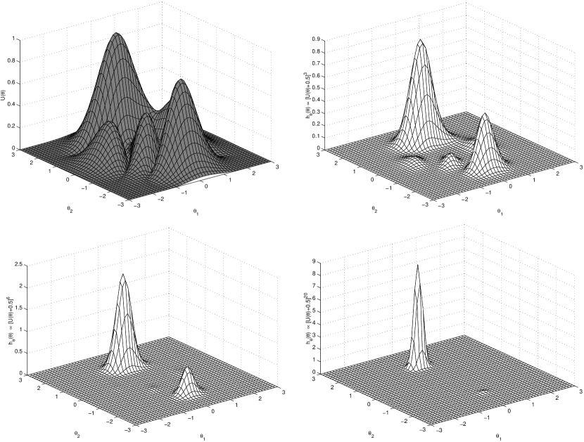
Figure 1: The function $U(\theta)$ (upper left) and some probability densities of the form $h_{\bm{\theta}}(\theta)\propto[U(\theta)+\delta]^{J}$ for $\delta=0.5$ and $J=3$ (upper right), $J=6$ (lower left) and $J=20$ (lower right).

In the generic formulation of the method, the Markov transition kernel of the $k$-th step of the inhomogeneous chain has equilibrium distribution $\pi^{(J_{k})}$ where $\{J_{k}\}_{k=1,2,\dots}$ is the “cooling schedule”. The cooling schedule is a non-decreasing sequence of positive numbers according to which the equilibrium distribution become increasingly sharpened during the evolution of the chain. We use $\bm{\theta}_{k}$ to denote the state of the chain and $P_{\bm{\theta}_{k}}$ to denote its probability distribution. The distribution $P_{\bm{\theta}_{k}}$ obviously depends on the initial condition $\bm{\theta}_{0}$. However, in this work, we don’t need to make this dependence explicit in the notation.

Remark 1: If, given an element $\theta$ in $\bm{\Theta}$, the value $U(\theta)$ can be computed directly, we say that $U$ is a deterministic criterion, e.g. the energy landscape in protein structure prediction [1]. In problems involving random variables, the value $U(\theta)$ may be the expected value $U(\theta)=\int g(x,\theta)p_{\bm{x}}(x;\theta)dx$ of some function $g$ which depends on both the optimization variable $\theta$, and on some random variable $\bm{x}$ which has probability density $p_{\bm{x}}(x;\theta)$ (which may itself depend on $\theta$). In such problems it is usually not possible to compute $U(\theta)$ directly, either because evaluation of the integral requires too much computation, or because no analytical expression for $p_{\bm{x}}(x;\theta)$ is available. Typically one must perform stochastic simulations in order to obtain samples of $\bm{x}$ for a given $\theta$, hence obtain sample values of $g(\bm{x},\theta)$, and thus construct a Monte Carlo estimate of $U(\theta)$. The Bayesian design of clinical trials is an important application area where such expected-value criteria arise [23]. The authors of this paper investigate the optimization of expected-value criteria motivated by problems of aircraft routing [24]. In the particular case that $p_{\bm{x}}(x;\theta)$ does not depend on $\theta$, the optimization task is often called “empirical risk minimization”, and is studied extensively in statistical learning theory [16, 17]. The results of this paper apply in the same way to the optimization of both deterministic and expected-value criteria. The MCMC method developed by Müller [25, 26] allows one to construct simulated annealing algorithms for the optimization of expected-value criteria. Müller [25, 26] employs the same equilibrium distributions as those described in our setting; in his context $J$ is restricted to integer values.

In Figure 2, we illustrate the basic iteration of a generic simulated annealing algorithm with equilibrium distributions $\pi^{(J)}(d\theta)$ for the optimization of deterministic and expected-value criteria.

Figure 2: The basic iterations of simulated annealing with equilibrium distributions $\pi^{(J)}(d\theta)$, for the maximization of deterministic and expected-value criteria (see Remark 1). In the algorithms, $q_{\tilde{\bm{\theta}}}$ is the density of the “proposal distribution” of the Metropolis step. The iteration for the expected value criterion has been proposed by Müller [25, 26].

2 Convergence

The rationale of simulated annealing is as follows: if the temperature is kept constant, say $J_{k}=J$, then the distribution of the state of the chain $P_{\bm{\theta}_{k}}$ tends to the equilibrium distribution $\pi^{(J)}$; if $J\rightarrow\infty$ then the equilibrium distribution $\pi^{(J)}$ tends to the zero-temperature distribution $\pi^{(\infty)}$; as a result, if the cooling schedule $J_{k}$ tends to infinity, one obtains that $P_{\bm{\theta}_{k}}$ “follows” $\pi^{(J_{k})}$ and that $\pi^{(J_{k})}$ tends to $\pi^{(\infty)}$ and eventually that the distribution of the state of the chain $P_{\bm{\theta}_{k}}$ tends to $\pi^{(\infty)}$. The theory shows that, under conditions on the cooling schedule and the Markov transition kernels, the distribution of the state of the chain $P_{\bm{\theta}_{k}}$ actually converges to the target zero-temperature distribution $\pi^{(\infty)}$ as $k\rightarrow\infty$ [12, 13, 14, 15]. Convergence to the zero-temperature distribution implies that asymptotically the state of the chain eventually coincides with a global optimizer with probability one.

The difficulty which must be overcome in order to obtain finite step results on simulated annealing algorithms on a continuous domain is that usually, in an optimization problem defined over continuous variables, the set of global optimizers has zero Lebesgue measure (e.g. a set of isolated points). If the set of global optimizers has zero measure then the set of global optimizers has null probability according to the equilibrium distributions $\pi^{(J)}$ for any finite $J$ and, as a consequence, according to the distributions $P_{\bm{\theta}_{k}}$ for any finite $k$. Put another way, the probability that the state of the chain visits the set of global optimizers is constantly zero after any finite number of steps. Hence the confidence of the fact that the solution provided by the algorithm in finite time coincides with a global optimizer is also constantly zero. Notice that this is not the case for a finite domain, where the set of global optimizers is of non-null measure with respect to the reference counting measure [7, 8, 9, 10].

It is instructive to look at the issue also in terms of the rate of convergence to the target zero-temperature distribution. On a discrete domain, the distribution of the state of the chain at each step and the zero-temperature distribution are both standard discrete distributions. It is then possible to define a distance between them and study the rate of convergence of this distance to zero. This analysis allows one to obtain results on the finite-time behavior of simulated annealing [7, 8]. On a continuous domain and for a set of global optimizers of measure zero, the target zero-temperature distribution $\pi^{(\infty)}$ ends up being a mixture of probability masses on the set of global optimizers. In this situation, although the distribution of the state of the chain $P_{\bm{\theta}_{k}}$ still converges asymptotically to $\pi^{(\infty)}$, it is not possible to introduce a sensible distance between the two distributions and a rate of convergence to the target distribution cannot even be defined (weak convergence), see [12, Theorem 3.3]. This is the reason that until now there have been no guarantees on the performance of simulated annealing on a continuous domain after a finite number of computations: by adopting the zero-temperature distribution $\pi^{(\infty)}$ as the target distribution it is only possible to prove asymptotic convergence in infinite time to a global optimizer.

Remark 2: The standard distance between two distributions, say $\mu_{1}$ and $\mu_{2}$, on a continuous support is the total variation norm $\|\mu_{1}-\mu_{2}\|_{TV}=\sup_{A}|\mu_{1}(A)-\mu_{2}(A)|$, see e.g. [21]. In simulated annealing on a continuous domain the distribution of the state of the chain $P_{\bm{\theta}_{k}}$ is absolutely continuous with respect to the Lebesgue measure (i.e. $\pi_{Leb}(A)=0\Rightarrow P_{\bm{\theta}_{k}}(A)=0$), by construction for any finite $k$. Hence if the set of global optimizers has zero Lebesgue measure then it has zero measure also according to $P_{\bm{\theta}_{k}}$. The set of global optimizers has however measure 1 according to $\pi^{(\infty)}$. The distance $\|P_{\bm{\theta}_{k}}-\pi^{(\infty)}\|_{TV}$ is then constantly $1$ for any finite $k$.

It is also worth mentioning that if the set of global optimizers has zero measure then asymptotic convergence to the zero-temperature distribution $\pi^{(\infty)}$ can be proven only under the additional assumptions of continuity and differentiability of $U$ [12, 13, 14, 15].

3 Finite-time guarantees

In general, optimization algorithms for problems defined on continuous variables can only find approximate solutions in finite time [27]. Given an element $\theta$ of a continuous domain how can we assess how good it is as an approximate solution to an optimization problem? Here we introduce the concept of approximate global optimizer to answer this question. The definition is given for a maximization problem in a continuous but bounded domain. We use two parameters: the value imprecision $\epsilon$ (greater than or equal to 0) and the residual domain $\alpha$ (between 0 and 1) which together determine the level of approximation. We say that $\theta$ is an approximate global optimizer of $U$ with value imprecision $\epsilon$ and residual domain $\alpha$ if the function $U$ takes values strictly greater than $U(\theta)+\epsilon$ only on a subset of values of $\theta$ no larger than an $\alpha$ portion of the optimization domain. The formal definition is as follows.

Definition 1

Let $U:\bm{\Theta}\rightarrow\mathbb{R}$ be an optimization criterion where $\bm{\Theta}\subset\mathbb{R}^{N}$ is bounded. Let $\pi_{Leb}$ denote the standard Lebesgue measure. Let $\epsilon\geq 0$ and $\alpha\in[0,\,1]$ be given numbers. Then $\theta$ is an approximate global optimizer of $U$ with value imprecision $\epsilon$ and residual domain $\alpha$ if $\pi_{Leb}\{\theta^{\prime}\in\bm{\Theta}:U(\theta^{\prime})>U(\theta)+\epsilon\}\leq\alpha\,\pi_{Leb}(\bm{\Theta})\,.$

In other words, the value $U(\theta)$ is within $\epsilon$ of a value which is greater than the values that $U$ takes on at least a $1-\alpha$ portion of the domain. The smaller $\epsilon$ and $\alpha$ are, the better is the approximation of a true global optimizer. If both $\alpha$ and $\epsilon$ are equal to zero then $U(\theta)$ coincides with the essential supremum of $U$.

Our definition of approximate global optimizer carries an important property, which holds regardless of what the criterion $U$ is: if $\epsilon$ and $\alpha$ have non-zero values then the set of approximate global optimizers always has non-zero Lebesgue measure. It follows that the probability that the chain visits the set of approximate global optimizers can be non-zero. Hence, it is sensible to study the confidence of the fact that the solution found by simulated annealing in finite time is an approximate global optimizer.

Remark 3: The intuition that our notion of approximate global optimizer can be used to obtain formal guarantees on the finite-time performance of optimization methods based on a stochastic search of the domain is already apparent in the work of Vidyasagar [17, 28]. Vidyasagar [17, 28] introduces a similar definition and obtains rigorous finite-time guarantees in the optimization of expected value criteria based on uniform independent sampling of the domain. Notably, the number of independent samples required to guarantee some desired accuracy and confidence turns out to be polynomial in the values of the desired imprecision, residual domain and confidence. Although the method of Vidyasagar is not highly sophisticated, it has had considerable success in solving difficult control system design applications [28, 29]. Its appeal stems from its rigorous finite-time guarantees which exist without the need for any particular assumption on the optimization criterion.

Here we show that finite-time guarantees for simulated annealing can be obtained by selecting a distribution $\pi^{(J)}$ with a finite $J$ as the target distribution in place of the zero-temperature distribution $\pi^{(\infty)}$. The fundamental result is the following theorem which allows one to select in a rigorous way $\delta$ and $J$ in the target distribution $\pi^{(J)}$. It is important to stress that the result holds universally for any optimization criterion $U$ on a bounded domain. The only minor requirement is that $U$ takes values in $[0,\,1]$.

Theorem 1

Let $U:\bm{\Theta}\rightarrow[0,\,1]$ be an optimization criterion where $\bm{\Theta}\subset\mathbb{R}^{N}$ is bounded. Let $J\geq 1$ and $\delta>0$ be given numbers. Let $\bm{\theta}$ be a multivariate random variable with distribution $\pi^{(J)}(d\theta)\propto[U(\theta)+\delta]^{J}\pi_{Leb}(d\theta)$. Let $\alpha\in(0,\,1]$ and $\epsilon\in[0,\,1]$ be given numbers and define

$$\sigma=\frac{1}{\mbox{$\displaystyle 1+\left[\frac{1+\delta}{\epsilon+1+\delta}\right]^{\,J}\left[\frac{1}{\alpha}\frac{1+\delta}{\epsilon+\delta}-1\right]\frac{1+\delta}{\delta}$}}\,\,.$$ (1)

Then the statement “$\bm{\theta}$ is an approximate global optimizer of $U$ with value imprecision $\epsilon$ and residual domain $\alpha$” holds with probability at least $\sigma$.

Proof. See Appendix A.

The importance of the choice of a target distribution $\pi^{(J)}$ with a finite $J$ is that $\pi^{(J)}$ is absolutely continuous with respect to the Lebesgue measure. Hence, the distance $\|P_{\bm{\theta}_{k}}-\pi^{(J)}\|_{\mbox{TV}}$ between the distribution of the state of the chain $P_{\bm{\theta}_{k}}$ and the target distribution $\pi^{(J)}$ is a meaningful quantity.

Convergence of the Metropolis-Hastings algorithm and MCMC methods in total variation norm is a well studied problem. The theory provides simple conditions under which one derives upper bounds on the distance to the target distribution which are known at each step of the chain and decrease monotonically to zero as the number of steps of the chain grows. The theory has been developed mainly for homogeneous chains [18, 19, 20, 21].

In the case of simulated annealing, the factor that enables us to employ these results is the absolute continuity of the target distribution $\pi^{(J)}$ with respect to the Lebesgue measure. However, simulated annealing involves the simulation of inhomogeneous chains. In this respect, another important fact is that the choice of a target distribution $\pi^{(J)}$ with a finite $J$ implies that the inhomogeneous Markov chain can in fact be formed by a finite sequence of homogeneous chains (i.e. the cooling schedule $\{J_{k}\}_{k=1,2,\dots}$ can be chosen to be a sequence that takes only a finite set of values). In turn, this allows one to apply the theory of homogeneous MCMC methods to study the convergence of $P_{\bm{\theta}_{k}}$ to $\pi^{(J)}$ in total variation norm.

On a bounded domain, simple conditions on the ‘proposal distribution’ in the iteration of the simulated annealing algorithm allows one to obtain upper bounds on $\|P_{\bm{\theta}_{k}}-\pi^{(J)}\|_{\mbox{TV}}$ that decrease geometrically to zero as $k\rightarrow\infty$, without the need for any additional assumption on $U$ [18, 19, 20, 21].

It is then appropriate to introduce the following finite-time result.

Theorem 2

Let the notation and assumptions of Theorem 1 hold. Let $\bm{\theta}_{k}$, with distribution $P_{\bm{\theta}_{k}}$, be the state of the inhomogeneous chain of a simulated annealing algorithm with target distribution $\pi^{(J)}$. Then the statement “$\bm{\theta}_{k}$ is an approximate global optimizer of $U$ with value imprecision $\epsilon$ and residual domain $\alpha$” holds with probability at least $\sigma-\|P_{\bm{\theta}_{k}}-\pi^{(J)}\|_{\mbox{TV}}$.

The proof of the theorem follows directly from the definition of the total variation norm.

It follows that if simulated annealing is implemented with an algorithm which converges in total variation distance to a target distribution $\pi^{(J)}$ with a finite $J$, then one can state with confidence arbitrarily close to 1 that the solution found by the algorithm after the known appropriate finite number of steps is an approximate global optimizer with the desired approximation level. For given non-zero values of $\epsilon$, $\alpha$ the value of $\sigma$ given by (1) can be made arbitrarily close to 1 by choice of $J$; while the distance $\|P_{\bm{\theta}_{k}}-\pi^{(J)}\|_{\mbox{TV}}$ can be made arbitrarily small by taking the known sufficient number of steps.

It can be shown that there exists the possibility of making an optimal choice of $\delta$ and $J$ in the target distribution $\pi^{(J)}$. In fact, for given $\epsilon$ and $\alpha$ and a given value of $J$ there exists an optimal choice of $\delta$ which maximizes the value of $\sigma$ given by (1). Hence, it is possible to obtain a desired $\sigma$ with the smallest possible $J$. The advantage of choosing the smallest $J$, consistent with the required approximation and confidence, is that it will decrease the number of steps required to achieve the desired reduction of $\|P_{\bm{\theta}_{k}}-\pi^{(J)}\|_{\mbox{TV}}$.

4 Conclusions

We have introduced a new formulation of simulated annealing which admits rigorous finite-time guarantees in the optimization of functions of continuous variables. First, we have introduced the notion of approximate global optimizer. Then, we have shown that simulated annealing is guaranteed to find approximate global optimizers, with the desired confidence and the desired level of accuracy, in a known finite number of steps, if a proper choice of the target distribution is made and conditions for convergence in total variation norm are met. The results hold for any optimization criterion on a bounded domain with the only minor requirement that it takes values between 0 and 1.

In this framework, simulated annealing algorithms with rigorous finite-time guarantees can be derived by studying the choice of the proposal distribution and of the cooling schedule, in the generic iteration of simulated annealing, in order to ensure convergence to the target distribution in total variation norm. To do this, existing theory of convergence of the Metropolis-Hastings algorithm and MCMC methods on continuous domains can be used [18, 19, 20, 21].

Vidyasagar [17, 28] has introduced a similar definition of approximate global optimizer and has shown that approximate optimizers with desired accuracy and confidence can be obtained with a number of uniform independent samples of the domain which is polynomial in the accuracy and confidence parameters. In general, algorithms developed with the MCMC methodology can be expected to be equally or more efficient than uniform independent sampling.

Acknowledgments

Work supported by EPSRC, Grant EP/C014006/1, and by the European Commission under projects HYGEIA FP6-NEST-4995 and iFly FP6-TREN-037180. We thank S. Brooks, M. Vidyasagar and D. M. Wolpert for discussions and useful comments on the paper.

Appendix A Proof of Theorem 1

Let $\bar{\alpha}\in(0,\,1]$ and $\rho\in(0,\,1]$ be given numbers. Let $U_{\delta}(\theta):=U(\theta)+\delta$. Let $\pi_{\delta}$ be a normalized measure such that $\pi_{\delta}(d\theta)\propto U_{\delta}(\theta)\pi_{Leb}(d\theta)$. In the first part of the proof we find a lower bound on the probability that $\bm{\theta}$ belongs to the set

$$\{\theta\in\bm{\Theta}:\pi_{\delta}\{\theta^{\prime}\in\bm{\Theta}:\rho\,U_{\delta}(\theta^{\prime})>U_{\delta}(\theta)\}\leq\bar{\alpha}\}\,.$$

Let $y_{\bar{\alpha}}:=\inf\{y:\pi_{\delta}\{\theta\in\bm{\Theta}:U_{\delta}(\theta)\leq y\}\geq 1-\bar{\alpha}\}$. To start with we show that the set $\{\theta\in\bm{\Theta}:\pi_{\delta}\{\theta^{\prime}\in\bm{\Theta}:\rho\,U_{\delta}(\theta^{\prime})>U_{\delta}(\theta)\}\leq\bar{\alpha}\}$ coincides with $\{\theta\in\bm{\Theta}:U_{\delta}(\theta)\geq\rho\,y_{\bar{\alpha}}\}$. Notice that the quantity $\pi_{\delta}\{\theta\in\bm{\Theta}:U_{\delta}(\theta)\leq y\}$ is a right-continuous non-decreasing function of $y$ because it has the form of a distribution function (see e.g. [30, p.162] and [17, Lemma 11.1]). Therefore we have $\pi_{\delta}\{\theta\in\bm{\Theta}:U_{\delta}(\theta)\leq y_{\bar{\alpha}}\}\geq 1-\bar{\alpha}$ and

$$y\geq\rho\,y_{\bar{\alpha}}\quad\Rightarrow\quad\pi_{\delta}\{\theta^{\prime}\in\bm{\Theta}:\rho\,U_{\delta}(\theta^{\prime})\leq y\}\geq 1-\bar{\alpha}\quad\Rightarrow\quad\pi_{\delta}\{\theta^{\prime}\in\bm{\Theta}:\rho\,U_{\delta}(\theta^{\prime})>y\}\leq\bar{\alpha}\,.$$

Moreover,

$$y<\rho\,y_{\bar{\alpha}}\quad\Rightarrow\quad\pi_{\delta}\{\theta^{\prime}\in\bm{\Theta}:\rho\,U_{\delta}(\theta^{\prime})\leq y\}<1-\bar{\alpha}\quad\Rightarrow\quad\pi_{\delta}\{\theta^{\prime}\in\bm{\Theta}:\rho\,U_{\delta}(\theta^{\prime})>y\}>\bar{\alpha}$$

and taking the contrapositive one obtains

$$\pi_{\delta}\{\theta^{\prime}\in\bm{\Theta}:\rho\,U_{\delta}(\theta^{\prime})>y\}\leq\bar{\alpha}\quad\Rightarrow\quad y\geq\rho\,y_{\bar{\alpha}}.$$

Therefore $\{\theta\in\bm{\Theta}:U_{\delta}(\theta)\geq\rho\,y_{\bar{\alpha}}\}\equiv\{\theta\in\bm{\Theta}:\pi_{\delta}\{\theta^{\prime}\in\bm{\Theta}:\rho\,U_{\delta}(\theta^{\prime})>U_{\delta}(\theta)\}\leq\bar{\alpha}\}$. We now derive a lower bound on $\pi^{(J)}\{\theta\in\bm{\Theta}:U_{\delta}(\theta)\geq\rho\,y_{\bar{\alpha}}\}$. Let us introduce the notation $A_{\bar{\alpha}}:=\{\theta\in\bm{\Theta}:U_{\delta}(\theta)<y_{\bar{\alpha}}\}$, $\bar{A}_{\bar{\alpha}}:=\{\theta\in\bm{\Theta}:U_{\delta}(\theta)\geq y_{\bar{\alpha}}\}$, $B_{\bar{\alpha},\rho}:=\{\theta\in\bm{\Theta}:U_{\delta}(\theta)<\rho\,y_{\bar{\alpha}}\}$ and $\bar{B}_{\bar{\alpha},\rho}:=\{\theta\in\bm{\Theta}:U_{\delta}(\theta)\geq\rho\,y_{\bar{\alpha}}\}$. Notice that $B_{\bar{\alpha},\rho}\subseteq A_{\bar{\alpha}}$ and $\bar{A}_{\bar{\alpha}}\subseteq\bar{B}_{\bar{\alpha},\rho}$. The quantity $\pi_{\delta}\{\theta\in\bm{\Theta}:U_{\delta}(\theta)<y\}$ as a function of $y$ is the left-continuous version of $\pi_{\delta}\{\theta\in\bm{\Theta}:U_{\delta}(\theta)\leq y\}$[30, p.162]. Hence, the definition of $y_{\bar{\alpha}}$ implies $\pi_{\delta}(A_{\bar{\alpha}})\leq 1-\bar{\alpha}$ and $\pi_{\delta}(\bar{A}_{\bar{\alpha}})\geq\bar{\alpha}$. Notice that

$$\pi_{\delta}(A_{\bar{\alpha}})\leq 1-\bar{\alpha}\quad \Rightarrow\quad\frac{\delta\pi_{Leb}(A_{\bar{\alpha}})}{\left[\int_{\bm{\Theta}}U_{\delta}(\theta)\pi_{Leb}(d\theta)\right]}\leq 1-\bar{\alpha}\,,$$

$$\pi_{\delta}(\bar{A}_{\bar{\alpha}})\geq\bar{\alpha}\quad \Rightarrow\quad\frac{(1+\delta)\pi_{Leb}(\bar{A}_{\bar{\alpha}})}{\left[\int_{\bm{\Theta}}U_{\delta}(\theta)\pi_{Leb}(d\theta)\right]}\geq\bar{\alpha}\,.$$

Hence, ${\pi_{Leb}(\bar{A}_{\bar{\alpha}})}>0$ and

$$\frac{\pi_{Leb}(A_{\bar{\alpha}})}{\pi_{Leb}(\bar{A}_{\bar{\alpha}})}\leq\frac{1-\bar{\alpha}}{\bar{\alpha}}\frac{1+\delta}{\delta}\,.$$

Notice that ${\pi_{Leb}(\bar{A}_{\bar{\alpha}})}>0$ implies ${\pi_{Leb}(\bar{B}_{\bar{\alpha},\rho})}>0$. We obtain

$$\pi^{(J)}\{\theta\in\bm{\Theta}:U_{\delta}(\theta)\geq\rho\,y_{\bar{\alpha}}\}=\frac{1}{\mbox{$\displaystyle 1+\frac{\int_{B_{\bar{\alpha},\rho}}U_{\delta}(\theta)^{J}\pi_{Leb}(d\theta)}{\int_{\bar{B}_{\bar{\alpha},\rho}}U_{\delta}(\theta)^{J}\pi_{Leb}(d\theta)}$}}$$

$$\geq\frac{1}{\mbox{$\displaystyle 1+\frac{\int_{B_{\bar{\alpha},\rho}}U_{\delta}(\theta)^{J}\pi_{Leb}(d\theta)}{\int_{\bar{A}_{\bar{\alpha}}}U_{\delta}(\theta)^{J}\pi_{Leb}(d\theta)}$}}\geq\frac{1}{\mbox{$\displaystyle 1+\frac{\rho^{\,J}y_{\bar{\alpha}}^{J}}{y_{\bar{\alpha}}^{J}}\frac{\pi_{Leb}(B_{\bar{\alpha},\rho})}{\pi_{Leb}(\bar{A}_{\bar{\alpha}})}$}}$$

$$\geq\frac{1}{\mbox{$\displaystyle 1+\rho^{\,J}\frac{\pi_{Leb}(A_{\bar{\alpha}})}{\pi_{Leb}(\bar{A}_{\bar{\alpha}})}$}}\geq\frac{1}{\mbox{$\displaystyle 1+\rho^{\,J}\frac{1-\bar{\alpha}}{\bar{\alpha}}\frac{1+\delta}{\delta}$}}\,.$$

Since $\{\theta\in\bm{\Theta}:U_{\delta}(\theta)\geq\rho\,y_{\bar{\alpha}}\}\equiv\{\theta\in\bm{\Theta}:\pi_{\delta}\{\theta^{\prime}\in\bm{\Theta}:\rho\,U_{\delta}(\theta^{\prime})>U_{\delta}(\theta)\}\leq\bar{\alpha}\}$ the first part of the proof is complete.

In the second part of the proof we show that the set $\{\theta\in\bm{\Theta}:\pi_{\delta}\{\theta^{\prime}\in\bm{\Theta}:\rho\,U_{\delta}(\theta^{\prime})>U_{\delta}(\theta)\}\leq\bar{\alpha}\}$ is contained in the set of approximate global optimizers of $U$ with value imprecision $\tilde{\epsilon}:=(\rho^{-1}-1)(1+\delta)$ and residual domain $\tilde{\alpha}:=\frac{1+\delta}{\tilde{\epsilon}+\delta}\,\bar{\alpha}$. Hence, we show that $\{\theta\in\bm{\Theta}:\pi_{\delta}\{\theta^{\prime}\in\bm{\Theta}:\rho\,U_{\delta}(\theta^{\prime})>U_{\delta}(\theta)\}\leq\bar{\alpha}\}\subseteq\{\theta\in\bm{\Theta}:\pi_{Leb}\{\theta^{\prime}\in\bm{\Theta}:U(\theta^{\prime})>U(\theta)+\tilde{\epsilon}\}\leq\tilde{\alpha}\,\pi_{Leb}(\bm{\Theta})\}.$ We have

$$U(\theta^{\prime})>U(\theta)+\tilde{\epsilon}\quad\Leftrightarrow\quad\rho\,U_{\delta}(\theta^{\prime})>\rho\,[U_{\delta}(\theta)+\tilde{\epsilon}]\quad\Rightarrow\quad\rho\,U_{\delta}(\theta^{\prime})>U_{\delta}(\theta)$$

which is proven by noticing that $\rho\,[U_{\delta}(\theta)+\tilde{\epsilon}]\geq U_{\delta}(\theta)\,\,\Leftrightarrow\,\,1-\rho\geq U(\theta)(1-\rho)$and $U(\theta)\in[0,\,1]$. Hence $\{\theta^{\prime}\in\bm{\Theta}:\rho\,U_{\delta}(\theta^{\prime})>U_{\delta}(\theta)\}\,\supseteq\,\{\theta^{\prime}\in\bm{\Theta}:U(\theta^{\prime})>U(\theta)+\tilde{\epsilon}\}\,.$ Therefore $\pi_{\delta}\{\theta^{\prime}\in\bm{\Theta}:\rho\,U_{\delta}(\theta^{\prime})>U_{\delta}(\theta)\}\leq\bar{\alpha}\,\Rightarrow\,\pi_{\delta}\{\theta^{\prime}\in\bm{\Theta}:U(\theta^{\prime})>U(\theta)+\tilde{\epsilon}\}\leq\bar{\alpha}\,.$ Let $Q_{\theta,\tilde{\epsilon}}:=\{\theta^{\prime}\in\bm{\Theta}:U(\theta^{\prime})>U(\theta)+\tilde{\epsilon}\}$ and notice that

$$\pi_{\delta}\{\theta^{\prime}\in\bm{\Theta}:U(\theta^{\prime})>U(\theta)+\tilde{\epsilon}\}=\frac{\mbox{$\displaystyle\int_{Q_{\theta,\tilde{\epsilon}}}U(\theta^{\prime})\pi_{Leb}(d\theta^{\prime})+\delta\pi_{Leb}(Q_{\theta,\tilde{\epsilon}})$}}{\mbox{$\displaystyle\int_{\bm{\Theta}}U(\theta^{\prime})\pi_{Leb}(d\theta^{\prime})+\delta\pi_{Leb}(\bm{\Theta})$}}\,.$$

We obtain

$$\pi_{\delta}\{\theta^{\prime}\in\bm{\Theta}:U(\theta^{\prime})>U(\theta)+\tilde{\epsilon}\}\leq\bar{\alpha} \Rightarrow\,\tilde{\epsilon}\,\pi_{Leb}(Q_{\theta,\tilde{\epsilon}})+\delta\pi_{Leb}(Q_{\theta,\tilde{\epsilon}})\leq\bar{\alpha}(1+\delta)\pi_{Leb}(\bm{\Theta})$$

$$\Rightarrow\,\pi_{Leb}\{\theta^{\prime}\in\bm{\Theta}:U(\theta^{\prime})>U(\theta)+\tilde{\epsilon}\}\leq\tilde{\alpha}\,\pi_{Leb}(\bm{\Theta})\,.$$

Hence we can conclude that

$$\pi_{\delta}\{\theta^{\prime}\in\bm{\Theta}:\rho\,U_{\delta}(\theta^{\prime})>U_{\delta}(\theta)\}\leq\bar{\alpha}\,\,\Rightarrow\,\,\pi_{Leb}\{\theta^{\prime}\in\bm{\Theta}:U(\theta^{\prime})>U(\theta)+\tilde{\epsilon}\}\leq\tilde{\alpha}\,\pi_{Leb}(\bm{\Theta})$$

and the second part of the proof is complete.

We have shown that given $\bar{\alpha}\in(0,\,1]$, $\rho\in(0,\,1]$, $\tilde{\epsilon}:=(\rho^{-1}-1)(1+\delta)$, $\tilde{\alpha}:=\frac{1+\delta}{\tilde{\epsilon}+\delta}\,\bar{\alpha}$ and

$$\sigma:=\frac{1}{\mbox{$\displaystyle 1+\rho^{\,J}\frac{1-\bar{\alpha}}{\bar{\alpha}}\frac{1+\delta}{\delta}$}}=\frac{1}{\mbox{$\displaystyle 1+\left[\frac{1+\delta}{\tilde{\epsilon}+1+\delta}\right]^{\,J}\left[\frac{1}{\tilde{\alpha}}\frac{1+\delta}{\tilde{\epsilon}+\delta}-1\right]\frac{1+\delta}{\delta}$}}\,,$$

the statement “$\bm{\theta}$ is an approximate global optimizer of $U$ with value imprecision $\tilde{\epsilon}$ and residual domain $\tilde{\alpha}$” holds with probability at least $\sigma$. Notice that $\tilde{\epsilon}\in[0,\,1]$ and $\tilde{\alpha}\in(0,\,1]$ are linked through a bijective relation to $\rho\in[\frac{1+\delta}{2+\delta},\,1]$ and $\bar{\alpha}\in(0,\,\frac{\tilde{\epsilon}+\delta}{1+\delta}]$. The statement of the theorem is eventually obtained by expressing $\sigma$ as a function of desired $\tilde{\epsilon}=\epsilon$ and $\tilde{\alpha}=\alpha$. $\Box$

References

- [1] D. J. Wales. Energy Landscapes. Cambridge University Press, Cambridge, UK, 2003.
- [2] D. Achlioptas, A. Naor, and Y. Peres. Rigorous location of phase transitions in hard optimization problems. Nature, 435:759–764, 2005.
- [3] S. Kirkpatrick, C. D. Gelatt, and M. P. Vecchi. Optimization by Simulated Annealing. Science, 220(4598):671–680, 1983.
- [4] E. Bonomi and J. Lutton. The -city travelling salesman problem: statistical mechanics and the Metropolis algorithm. SIAM Rev., 26(4):551–568, 1984.
- [5] Y. Fu and P. W. Anderson. Application of statistical mechanics to NP-complete problems in combinatorial optimization. J. Phys. A: Math. Gen., 19(9):1605–1620, 1986.
- [6] M. Mézard, G. Parisi, and R. Zecchina. Analytic and Algorithmic Solution of Random Satisfiability Problems. Science, 297:812–815, 2002.
- [7] P. M. J. van Laarhoven and E. H. L. Aarts. Simulated Annealing: Theory and Applications. D. Reidel Publishing Company, Dordrecht, Holland, 1987.
- [8] D. Mitra, F. Romeo, and A. Sangiovanni-Vincentelli. Convergence and finite-time behavior of simulated annealing. Adv. Appl. Prob., 18:747–771, 1986.
- [9] B. Hajek. Cooling schedules for optimal annealing. Math. Oper. Res., 13:311–329, 1988.
- [10] J. Hannig, E. K. P. Chong, and S. R. Kulkarni. Relative Frequencies of Generalized Simulated Annealing. Math. Oper. Res., 31(1):199–216, 2006.
- [11] S. Boyd and L. Vandenberghe. Convex Optimization. Cambridge University Press, Cambridge, UK, 2004.
- [12] H. Haario and E. Saksman. Simulated annealing process in general state space. Adv. Appl. Prob., 23:866–893, 1991.
- [13] S. B. Gelfand and S. K. Mitter. Simulated Annealing Type Algorithms for Multivariate Optimization. Algorithmica, 6:419–436, 1991.
- [14] C. Tsallis and D. A. Stariolo. Generalized simulated annealing. Physica A, 233:395–406, 1996.
- [15] M. Locatelli. Simulated Annealing Algorithms for Continuous Global Optimization: Convergence Conditions. J. Optimiz. Theory App., 104(1):121–133, 2000.
- [16] V. N. Vapnik. The Nature of Statistical Learning Theory. Cambridge University Press, Springer, New York, US, 1995.
- [17] M. Vidyasagar. Learning and Generalization: With Application to Neural Networks. Springer-Verlag, London, second edition, 2003.
- [18] S. P. Meyn and R. L. Tweedie. Markov Chains and Stochastic Stability. Springer-Verlag, London, 1993.
- [19] J. S. Rosenthal. Minorization Conditions and Convergence Rates for Markov Chain Monte Carlo. J. Am. Stat. Assoc., 90(430):558–566, 1995.
- [20] K. L. Mengersen and R. L. Tweedie. Rates of convergence of the Hastings and Metropolis algorithm. Ann. Stat., 24(1):101–121, 1996.
- [21] G. O. Roberts and J. S. Rosenthal. General state space Markov chains and MCMC algorithms. Prob. Surv., 1:20–71, 2004.
- [22] C. P. Robert and G. Casella. Monte Carlo Statistical Methods. Springer-Verlag, New York, second edition, 2004.
- [23] D.J. Spiegelhalter, K.R. Abrams, and J.P. Myles. Bayesian approaches to clinical trials and health-care evaluation. John Wiley & Sons, Chichester, UK, 2004.
- [24] A. Lecchini-Visintini, W. Glover, J. Lygeros, and J. M. Maciejowski. Monte Carlo Optimization for Conflict Resolution in Air Traffic Control. IEEE Trans. Intell. Transp. Syst., 7(4):470–482, 2006.
- [25] P. Müller. Simulation based optimal design. In J. O. Berger, J. M. Bernardo, A. P. Dawid, and A. F. M. Smith, editors, Bayesian Statistics 6: proceedings of the Sixth Valencia International Meeting, pages 459–474. Oxford: Clarendon Press, 1999.
- [26] P. Müller, B. Sansó, and M. De Iorio. Optimal Bayesian design by Inhomogeneous Markov Chain Simulation. J. Am. Stat. Assoc., 99(467):788–798, 2004.
- [27] L. Blum, C. Cucker, M. Shub, and S. Smale. Complexity and Real Computation. Springer-Verlag, New York, 1998.
- [28] M. Vidyasagar. Randomized algorithms for robust controller synthesis using statistical learning theory. Automatica, 37(10):1515–1528, 2001.
- [29] R. Tempo, G. Calafiore, and F. Dabbene. Randomized Algorithms for Analysis and Control of Uncertain Systems. Springer-Verlag, London, 2005.
- [30] B.V. Gnedenko. Theory of Probability. Chelsea, New York, fourth edition, 1968.