Order 1 autoregressive process of finite length

Abstract

The stochastic processes of finite length defined by recurrence relations request additional relations specifying the first terms of the process analogously to the initial conditions for the differential equations. As a general rule, in time series theory one analyzes only stochastic processes of infinite length which need no such initial conditions and their properties are less difficult to be determined. In this paper we compare the properties of the order 1 autoregressive processes of finite and infinite length and we prove that the time series length has an important influence mainly if the serial correlation is significant. These different properties can manifest themselves as transient effects produced when a time series is numerically generated. We show that for an order 1 autoregressive process the transient behavior can be avoided if the first term is a Gaussian random variable with standard deviation equal to that of the theoretical infinite process and not to that of the white noise innovation.

I Introduction

The purpose of the statistical processing of time series is to find a stochastic model which can generate time series having the same statistical properties as the observed series. One of the most common statistical model is the autoregressive moving average (ARMA) process having many applications in economy, finance, signal theory, geophysics, etc. box1976 . Lately, especially the applications of the autoregressive (AR) models have become more frequent in physics as well. For example they are used in the analysis of the wind speed fluctuations hall2007 , radar signals gao2006 , climatic phenomena variability mar2004 , electroencephalographic activity liley2003 , heart interbeat time series guzman2003 , the daily temperature fluctuations kiraly2002 , X-ray emmision from the active galactic nuclei timmer2000 , sunspots variability palus1999 , etc. As a result of their simple mathematical properties and their direct physical interpretation, the realizations of AR(1) processes have been used as artificial series to analyze some numerical algorithms for monotonic trend removal vamos2007 , some surrogate data test for nonlinearity kugiu2002 or for renormalization group analysis blender2001 .

A stochastic process $\{X_{t},t=0,\pm 1,\pm 2,...\}$ is called autoregressive process of order $p$, denoted AR$(p)$, if $\{X_{t}\}$ is stationary and for any $t$ we have

$$X_{t}-\phi_{1}X_{t-1}-...-\phi_{p}X_{t-p}=Z_{t}~{},$$ (1)

where $\{Z_{t}\}$ is a Gaussian white noise with zero mean and variance $\sigma^{2}$, and $\phi_{1},\phi_{2},...,\phi_{p}$ are real constants. The above relation may be rewritten in the compact form $\phi(B)X_{t}=Z_{t}$ where

$$\phi(z)=1-\phi_{1}z-...-\phi_{p}z^{p}$$ (2)

and $B$ is the shift operator, $BX_{t}=X_{t-1}$. Equation (1) has a unique solution if the polynomial (2) does not vanish for $|z|=1$ brock1991 . If in addition $\phi(z)\neq 0$ for all $|z|<1$, then the process is causal, i.e., there exists a sequence of constants $\{\psi_{j}\}$ such that $\sum_{j=1}^{\infty}|\psi_{j}|<\infty$ and

$$X_{t}=\sum_{j=0}^{\infty}\psi_{j}Z_{t-j}~{},\qquad t=0,\pm 1,...$$ (3)

Hence, a causal process is characterized by the property that the random variable $X_{t}$ can be expressed only in terms of noises at previous moments and at the same moment. The properties of AR$(p)$ processes have been studied in detail and they are the basis of the linear stochastic theory of time series (brock1991 , brock1996 , Hamilt1994 ).

The stochastic process defined above is an idealized mathematical object which has no direct correspondent in practice. Each time series obtained by measurements is a sequence of real numbers $x_{t}$ and one makes the assumption that each of those numbers is a realization of a random variable $X_{t}$. To recover the statistical information regarding the stochastic process we need a large number of time series generated in the same conditions, a situation occurring rarely in practice. Usually we have only one single time series and the recognition of the stochastic process that generated it is very difficult. In addition the finite length (sometimes very short) of the data series render the problem even harder. Therefore it is important to analyze a finite stochastic process satisfying the same recurrence relation as the idealized infinite stochastic process (1).

In the following we analyze the properties of an AR$(1)$ stochastic process of finite length allowing us to make detailed analytical and numerical computations. We compare the results obtained with the ideal case of the infinite stochastic process and we discuss the conclusions which can be obtained from its power spectrum.

II AR(1) process

A stochastic AR(1) process is defined by the simplified form of the relation (1)

$$X_{t}=\phi X_{t-1}+Z_{t}~{}.$$ (4)

By definition an AR(1) process has an infinite length. In this case the polynomial (2) has the form $\phi(z)=1-\phi z$ and then the causality condition reduces to $|\phi|<1$. Because the relation (4) is so simple, we can analyze more directly the significance of this condition. By successively applying (4) $\tau$ times we obtain

$$X_{t}=Z_{t}+\phi Z_{t-1}+...+\phi^{\tau-1}Z_{t-\tau+1}+\phi^{\tau}X_{t-\tau}~{}.$$ (5)

Because the process $\{X_{t}\}$ is stationary, the random variables $X_{t}$ and $X_{t-\tau}$ have the same norm and then the norm of the last term in (5) is $\phi^{\tau}$ times the norm of the left term. So for any positive number $\varepsilon<1$, there exists $\tau>\ln\varepsilon/\ln|\phi|>0$ such that the last term from the right side can be neglected

$$X_{t}=Z_{t}+\phi Z_{t-1}+...+\phi^{\tau-1}Z_{t-\tau+1}+\mathcal{O}(\varepsilon)$$ (6)

for $\varepsilon\rightarrow 0$. This is the definition relation of a causal process (3) where $\psi_{j}=\phi^{j}$. From relation (6) one observes that the influence of the noise reduces as the time moves away from $t$.

In the nonstationary case $|\phi|=1$, all the terms in (5) have unitary coefficients and for any delay $\tau$ none of them can be neglected. Every random variable $X_{t}$ is an infinite sum of terms with the same norm, hence its norm is infinite.

II.1 Causal AR(1) process

In the following we analyze the basic properties of the causal stationary process AR$(1)$ using the relation (4). If we take the mean of this relation we obtain $E\left\{X_{t}\right\}=0.$ Its square is

$$X_{t}^{2}=\phi^{2}X_{t-1}^{2}+2\phi X_{t-1}Z_{t}+Z_{t}^{2}.$$

In accordance with relation (6) the random variables $X_{t-1}$ and $Z_{t}$ are independent, that is $E\left\{X_{t-1}Z_{t}\right\}=0$. If we take the mean of the last relation we obtain a relation between the variance of successive random variables

$$\sigma_{t}^{2}=\phi^{2}\sigma_{t-1}^{2}+\sigma^{2}.$$

Because the AR$\left(1\right)$ process is stationary, it follows that for every $t$ we have the same value for the variance $\sigma_{t}\equiv\sigma_{s}$ and then

$$\sigma_{s}^{2}=\frac{\sigma^{2}}{1-\phi^{2}}.$$ (7)

In order to compute the autocovariance function we multiply (4) with $X_{t-\tau}$ and we take the mean. Because the mean of $X_{t}$ vanishes and $E\left\{X_{t-1}Z_{t}\right\}=0$, we obtain

$$\gamma\left(\tau\right)\equiv E\left\{X_{t}X_{t-\tau}\right\}=\phi\gamma\left(\tau-1\right).$$

By applying successively this relation and taking into account that $\gamma\left(0\right)=\sigma_{s}^{2}$, we have

$$\gamma\left(\tau\right)=\sigma_{s}^{2}\phi^{\tau}~{}.$$ (8)

The spectral density is the Fourier transform of the autocovariance function

$$f\left(\nu\right)=\frac{1}{2\pi}\sum_{\tau=-\infty}^{\infty}e^{-2\pi i\tau\nu}\gamma\left(\tau\right),$$ (9)

where the positive number $\nu$ is the frequency. By direct calculation with $\gamma\left(\tau\right)$ given by (8) we obtain

$$f\left(\nu\right)=\frac{\sigma^{2}}{2\pi}\frac{1}{1-2\phi\cos 2\pi\nu+\phi^{2}}.$$ (10)

Due to the periodicity of this function, we reduce its domain of definition to the interval $\nu\in[0,0.5]$.

When $\phi\rightarrow 1$, the standard deviation $\sigma_{s}$ given by (7) and the covariance function $\gamma(\tau)$ given by (8) become both of them infinite. The spectral density (10) becomes infinite only for $\nu=0$.

II.2 Acausal AR(1) process

Let us analyze the basic properties for the stationary acausal AR$(1)$ process, that is when $|\phi|>1$ in (4). The relation (6) is no more true because now $\phi^{\tau}$ increases when $\tau$ increases. If we divide (5) by $\phi^{\tau}$, then

$$\phi^{-\tau}X_{t}=\phi^{-\tau}Z_{t}+\phi^{-\tau+1}Z_{t-1}+...+\phi^{-1}Z_{t-\tau+1}+X_{t-\tau}~{}.$$

For every positive $\varepsilon<1$, there exists $\tau>-\ln\varepsilon/\ln|\phi|>0$ such that the term from the left side can be neglected and then

$$X_{t-\tau}=-\phi^{-1}Z_{t-\tau+1}-...-\phi^{-\tau+1}Z_{t-1}-\phi^{-\tau}Z_{t}+\mathcal{O}(\varepsilon)$$ (11)

for $\varepsilon\rightarrow 0$. Hence, the random variable at moment $t-\tau$ can be expressed in terms of the noise values at the future moments. It means that the direction of this process is reversed to that of the causal process (3).

The same conclusion can be drawn from (4) if we write it in the form

$$X_{t-1}=\phi^{-1}X_{t}-\phi^{-1}Z_{t}~{}.$$

In this way we obtain a stationary causal process AR$(1)$ because $|\phi^{-1}|<1$, but in reverse temporal direction and with the variance of the noise $\phi^{-1}\sigma$. It means that the formulas for the acausal AR(1) process can be obtained from those for the causal one by replacing $\phi$ with $\phi^{-1}$ and $\sigma$ with $\phi^{-1}\sigma$. We shall derive these formulas directly as well in order to verify this assertion.

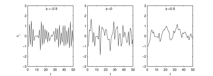
Figure 1: Realizations of an anticorrelated AR(1) process ($\phi=-0.9$), of an uncorrelated one ($\phi=0$), and of a correlated one ($\phi=0.9$).

From (11) it follows that the random variables $X_{t-1}$ and $Z_{t}$ are not independent, that is $E\left\{X_{t-1}Z_{t}\right\}\neq 0$. In this case $E\left\{X_{t}Z_{t}\right\}=0$, and then we write (4) in the form

$$\phi X_{t-1}=X_{t}-Z_{t}$$

and we square it

$$\phi^{2}X_{t-1}^{2}=X_{t}^{2}-2X_{t}Z_{t}+Z_{t}^{2}.$$

If we take the mean instead of (7) we obtain

$$\sigma_{s}^{2}=\frac{\sigma^{2}}{\phi^{2}-1}.$$

In order to compute the autocovariance function we multiply (4) by $X_{t+\tau}$ and instead of (8) we obtain

$$\gamma\left(\tau\right)=\sigma_{s}^{2}\phi^{-\tau}~{}.$$

Finally, relation (10) is the same.

II.3 Anticorrelated AR(1) process

Let us remark that the values of the parameter $\phi$ can be both positive and negative. In order to qualitatively characterize the difference between the two situations we use the fact that, if $\phi=0$, the AR(1) process is reduced to a white noise with uncorrelated terms and a vanishing autocovariance function for $\tau>0$. When $\phi>0$, from (4) it follows that the fluctuations due to the white noise are superposed over the term $|\phi|X_{t-1}$ which memorizes a part of the previous value of the time series. Hence, the larger $\phi$ is, the closer from each other the successive values of the time series are, and the fluctuations due to the white noise are smaller. Therefore, in comparison with a realization of a white noise, for $\phi>0$ the graphical representation of an AR(1) process is less fluctuant and resembles to a deterministic trajectory disturbed by a random fluctuation (see Fig. 1). The autocovariance function (8) is positive and tends to zero for $\tau\rightarrow\infty$.

If $\phi<0$, then the white noise is superposed over the term $-|\phi|X_{t-1}$ which has an opposite sign to the previous term of the time series. Consequently the white noise fluctuations are enhanced and the series values fluctuate with a larger amplitude than the white noise, as shown in Fig. 1. The successive values of the autocovariance function (8) are of opposite signs and the time series is called anticorrelated.

III AR(1) power spectrum

In Fig. 2 we have plotted the power spectrum (10) for $\phi=0.5$ and $\sigma=1$ on a linear scale and on a log-log one. The logarithmic coordinates strongly distort the shape of the graphic because by taking the logarithm, the origin of the Ox axis is send to $-\infty$ and any neighborhood of the origin is transformed into an infinite length interval. We have separated the graphic into three regions (A, B, and C) in order to evidence the deformations. For small frequencies (region A) the spectral density is strongly stretched such that a plateau appears with a value given by

$$f(0)=\frac{\sigma^{2}}{2\pi(1-\phi)^{2}}\ .$$ (12)

From relation (10) one observes that the plateau corresponds to the small values of $\nu$, when the variable term at the denominator can be neglected in comparison with the constant term. Using the quadratic approximation for cosine function we obtain the condition that the graph of the AR$(1)$ power spectrum has a plateau

$$\nu\ll\frac{1-\phi}{2\pi\sqrt{\phi}}.$$ (13)

One remarks that if $\phi$ tends to 1, then the plateau appears at smaller values of the frequency.

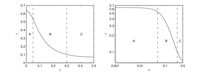
Figure 2: The power spectrum of an AR(1) process for $\phi=0.5$ and $\sigma=1$ on a linear scale and on a log-log one.

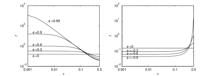
Figure 3: Power spectra of an AR(1) process for $\sigma=1$ and different values of $\phi$.

The region C of the spectral density for large frequencies is almost parallel to the $Ox$ axis in linear coordinates. In logarithmic coordinates it is strongly squeezed and acquires a significant slope. The region B of median frequencies is not compressed so much, but its almost exponential shape in linear coordinates becomes o curve with a considerable part having a constant slope. The relative length of the three frequency regions depends on the minimum value $\nu_{\min}$ of the frequency scale in the plot. If $\nu_{\min}$ is not small enough, then the plateau may remain outside the graphic.

As a global characteristic of the AR(1) power spectrum we introduce the difference of its extreme values, quantity which we call the spectrum amplitude and is denoted by $A$. For $\nu\in[0,0.5]$ the spectral density (10) is monotonic and its extreme values occur at $\nu=0$ and $\nu=0.5$. Using (12) and

$$f(0.5)=\frac{\sigma^{2}}{2\pi(1+\phi)^{2}}\ ,$$ (14)

we have for the spectrum amplitude

$$A=|f(0)-f(0.5)|=\frac{4|\phi|\sigma^{2}}{\left(1-\phi^{2}\right)^{2}}~{}.$$ (15)

The extreme values of the power spectrum (12) and (14) become equal for $\phi=0$ when the power spectrum is a line parallel with $Ox$ axis and $A=0$. One can see that for $\phi\rightarrow 1$, both $f(0)$ and $A$ tend to infinity.

In Fig. 3 we present the variation of the power spectrum with respect to $\phi$. Although in linear coordinates the power spectrum corresponding to $-\phi$ is the reflection of that corresponding to $\phi$ with respect to a line parallel to $Oy$ axis, in log-log scale they have very different shapes. This difference occurs because, as shown in Fig. 2, the small frequency region is stretched whereas that of large frequency is compressed. In accordance with (12), for $\phi>0$ the plateau height $f(0)$ increases with $\phi$ and the extreme region for large frequencies of the power spectrum $f(0.5)$ given by (14) has smaller values for smaller $\phi$.

From Fig. 3a and Fig. 2b it results that the AR(1) processes have some fractal features. For $\phi=0.9$ and especially for $\phi=0.99$, a large region of the power spectrum is linear with a slope near $-2$. Also for small values of $\phi$ (for example $\phi=0.5$ in Fig. 2b) a significant region of the power spectrum can be considered linear (fractal). In order to compute the slope of the power spectrum for arbitrary $\phi$, we denote by $\xi=\log x$ and $\eta=\log y$ the double-logarithmic coordinates such that a function $y=f\left(x\right)$ is written in the new coordinates as

$$\eta=\log_{10}f\left(10^{\xi}\right).$$

The slope of the log-log plot is

$$\beta\left(x\right)=\frac{d\eta}{d\xi}=-x\frac{d}{dx}\left(\ln f\left(x\right)\right).$$

If we apply this relation to the function (10), we obtain the slope of the AR(1) power spectrum

$$\beta(\nu;\phi)=-\frac{4\pi\phi\nu\sin 2\pi\nu}{1+\phi^{2}-2\phi\cos 2\pi\nu}\ .$$ (16)

In Fig. 4 we have plotted the absolute value of this function in log-log scale and we observe that for $\phi\gtrsim 0.9$ there exist values of $\beta$ near $-2$. We can verify this behavior substituting $\phi=1$ in (16)

$$\beta(\nu;1)=-2\pi\nu\cot\pi\nu\ .$$

Obviously this case is artificial because for $\phi=1$ we obtain the Brownian motion, not the AR(1) process. Then we have $\lim_{\nu\rightarrow 0}\beta(\nu;1)=-2$ which corresponds to the plateau in Fig. 4. If $\phi<1$, then $\beta(0;\phi)=0$ and in Fig. 4 the curve is decreasing for small frequencies. For $\phi<0.9$ there is only one maximum value for $\beta$ that corresponds to the center of the ”linear” (fractal) region of the power spectrum.

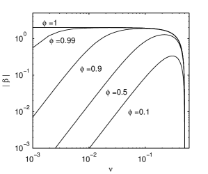
Figure 4: The absolute value of the slope of the AR(1) power spectrum for $\sigma=1$ and different values of $\phi$.

IV Finite AR(1) process

The time series appearing in practice have a finite length and usually they are considered finite samples of an AR(1) process of infinite length. The first terms of the sample are correlated with the preceding terms of the realization which has not been recorded. But the first terms of a numerically generated time series can not be related with realizations of other preceding random variables. Therefore, a numerically generated time series is never strictly a realization of a finite sample of an ideal stationary stochastic process of infinite length. For instance, the index $t$ in relations (1) and (4) cannot be an arbitrary integer. Because the relations defining the process are recursive, the first terms must be defined by additional relations. As we shall show in the following, the manner in which these additional relations are chosen can essentially modify the properties of the stochastic process. We shall call finite AR(1) process a stochastic process of finite length satisfying a recursive relation (1).

Let $T$ denote the length of a finite AR(1) process, that is $t=1,2,...,T$. The first term $X_{1}$ must be chosen independently and then we obtain another process instead of that studied in the previous section, denoted by $\{\widehat{X}_{t}\}$. Because $\widehat{X}_{t}$ satisfies the relation (4) for $t>1$, if we apply this relation successively we can express the terms of the stochastic process as a finite sum

$$\widehat{X}_{t}=Z_{t}+\phi Z_{t-1}+....+\phi^{t-2}Z_{2}+\phi^{t-1}\widehat{X}_{1}.$$ (17)

In the following we consider only the causal AR$(1)$ processes, i.e., we suppose $|\phi|<1$. As shown in the previous section, the acausal process is equivalent with a causal one generated in reverse order.

If $\widehat{X}_{1}$ is a Gaussian random variable with variance $\widehat{\sigma}_{1}$ and zero mean, then from (17) it follows that $\widehat{X}_{t}$ is the sum of $t$ Gaussian random variables, hence it has also a Gaussian distribution with variance

$$\widehat{\sigma}_{t}^{2}=\sigma^{2}\left(1+\phi^{2}+\phi^{4}+...+\phi^{2(t-2)}\right)+\widehat{\sigma}_{1}^{2}\phi^{2\left(t-1\right)}~{}.$$

Applying the formula for the sum of a geometric series we have

$$\widehat{\sigma}_{t}^{2}=\sigma_{s}^{2}+\left(\widehat{\sigma}_{1}^{2}-\sigma_{s}^{2}\right)\phi^{2\left(t-1\right)}~{},$$ (18)

where we have used (7). The variance of the finite AR(1) process has a constant term equal with the variance of the infinite AR(1) process (7) and a variable term which tends asymptotically to zero because $|\phi|<1$. In this case the finite AR(1) process is nonstationary presenting transient effects, i.e., its variance approximates the theoretical one $\widehat{\sigma}_{t}\simeq\sigma_{s}$ only after a time interval $t_{0}$ for which $\phi^{2t_{0}}$ can be neglected.

IV.1 Quasistationary finite AR(1) process

For $\widehat{\sigma}_{1}=\sigma_{s}$ the variable term in (18) vanishes and $\widehat{\sigma}_{t}=\sigma_{s}$ for all $t\leqslant T$. Hence, if for a finite AR(1) process we choose $\widehat{X}_{1}=(\sigma_{s}/\sigma)Z_{1}$, then all the terms have the same variance. This choice is natural because it is more reasonable to take the first term of the finite AR(1) process similar to the stationary infinite AR(1) process and not to the white noise. Because for $\widehat{\sigma}_{1}\neq\sigma_{s}$ the calculations become more complicated, we deal only with the case $\widehat{\sigma}_{1}=\sigma_{s}$.

Let us show that for $\widehat{\sigma}_{1}=\sigma_{s}$ the properties of the finite AR(1) process are very identical to those of a finite sample of a stationary infinite AR(1) process. The autocovariance function $\widehat{\gamma}(\tau;t)=E\{\widehat{X}_{t}\widehat{X}_{t-\tau}\}$ can be calculated only if $|\tau|<T$ and $\tau<t\leqslant T+\tau$. Unlike the autocovariance function (8) the quantity $\widehat{\gamma}\left(\tau;t\right)$ does not depend only on $\tau$ since it exists only for certain values of $t$. Therefore $\{\widehat{X}_{t}\}$ is not a stationary stochastic process in a strict mathematical meaning. However, when it exists, we can show that $E\{\widehat{X}_{t}\widehat{X}_{t-\tau}\}=\phi E\{\widehat{X}_{t-1}\widehat{X}_{t-\tau}\}$ proceeding in the same way as for (8). Then instead of (8) we obtain

$$\widehat{\gamma}\left(\tau;t\right)=\phi^{\tau}\widehat{\sigma}_{t-\tau}^{2}~{}.$$ (19)

If we choose $\widehat{\sigma}_{1}=\sigma_{s}$, then $\widehat{\sigma}_{t-\tau}=\sigma_{s}$ is constant and when $\widehat{\gamma}\left(\tau;t\right)$ exists it is identical to the covariance function $\gamma\left(\tau\right)$ in (8). Hence, if we want to numerically model a stationary infinite AR(1) process, then we have to use a finite AR(1) process $\{\widehat{X}_{t}\}$ with $\widehat{\sigma}_{1}=\sigma_{s}$.

IV.2 Brownian motion

Let us analyze now the finite AR(1) process satisfying (4) for $\phi=1$. This is the well known Brownian motion. In this case $\widehat{X}_{1}=Z_{1}$ and then (17) becomes

$$\widehat{X}_{t}=Z_{t}+Z_{t-1}+...+Z_{2}+Z_{1}.$$ (20)

Because $\widehat{X}_{t}$ is the sum of $t$ gaussian random variables, it results that its variance is the sum of the variances of the terms of the sum

$$\widehat{\sigma}_{t}^{2}=t\sigma^{2}.$$ (21)

If we write the relation (20) in the form

$$\widehat{X}_{t+\tau}=Z_{t+\tau}+...+Z_{t+1}+\widehat{X}_{t}~{},$$

multiply it with $\widehat{X}_{t}$ and take the mean, then we obtain

$$E\{\widehat{X}_{t+\tau}\widehat{X}_{t}\}=\widehat{\sigma}_{t}^{2}=t\sigma^{2}.$$ (22)

The relation between the Brownian motion and the quasistationary finite AR(1) process can be clarified if in (18) we take $\widehat{\sigma}_{1}=\sigma$ corresponding to the choice of the first term for the Brownian motion $\widehat{X}_{1}=Z_{1}$

$$\widehat{\sigma}_{t}^{2}=\sigma_{s}^{2}\left(1-\phi^{2t}\right)~{}.$$ (23)

Figure 4 shows the variation of $\widehat{\sigma}_{t}^{2}$ for different values of $\phi$. For a given $\phi$, at the beginning there is a nonstationary transient period before the stationary state of the AR(1) process is reached. As $\phi$ tends to $1$, the transient region is expanded and at the limit it becomes infinite, such that for $\phi=1$ an entirely nonstationary process is obtained, i.e., the Brownian motion. So the Brownian motion corresponds to the transient region extended to the infinity, whereas the stationary infinite AR(1) process corresponds to the stationary part of the graph. Therefore to obtain a quasistationary finite AR(1) process for $\phi$ very close to $1$ the only possibility is to choose $\widehat{\sigma}_{1}=\sigma_{s}$ completely eliminating the transient region.

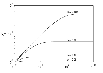
Figure 5: The standard deviation of a finite AR(1) process for different values of $\phi$ when the first term coincides with the white noise $\widehat{\sigma}_{1}=\sigma$. The transient region extends when $\phi$ takes greater values.

V Periodogram

For a finite AR(1) process the definition (9) can not be applied. Therefore we use the periodogram which is defined as the square of the absolute value of the discrete Fourier transform of the stochastic process of finite length stoica1997 . Here we consider only a finite equidistant set of frequencies for which we define the amplitude

$$A_{n}=\frac{1}{\sqrt{T}}\sum_{t=1}^{T}\widehat{X}_{t}\omega_{T}^{\left(t-1\right)\left(n-1\right)},\quad n=1,2,...,T,$$ (24)

where $\omega_{T}=\exp\left(-2\pi i/T\right)$. The corresponding terms of the periodogram are

$$I_{n}=\left|A_{n}\right|^{2}~{}.$$ (25)

Replacing (24) in (25) we have

$$I_{n}=\frac{1}{T}\sum_{t=1}^{T}\sum_{s=1}^{T}\widehat{X}_{t}\omega_{T}^{\left(t-1\right)\left(n-1\right)}\widehat{X}_{s}\omega_{T}^{-\left(s-1\right)\left(n-1\right)}~{}.$$

Because $\omega_{T}^{t-1}\omega_{T}^{-s+1}=\exp\left\{-\frac{2\pi i}{T}\left(t-s\right)\right\}$, we introduce a new variable $\tau=t-s$ and then

$$I_{n}=\frac{1}{T}\sum_{t=1}^{T}\widehat{X}_{t}^{2}+\frac{1}{T}\sum_{\tau=1}^{T-1}\left[\omega_{T}^{\tau\left(n-1\right)}+\omega_{T}^{-\tau\left(n-1\right)}\right]\sum_{t=1}^{T-\tau}\widehat{X}_{t}\widehat{X}_{t+\tau}.$$ (26)

The terms $I_{n}$ of the periodogram are random variables and their mean $E\left\{I_{n}\right\}$ tends to the spectral density $f(\nu)$ given by (10) when $T\rightarrow\infty$ brock1991 . We shall show this property only for the two particular cases considered in the previous section for which the calculations are shorter.

V.1 The periodogram of the quasistationary finite AR(1) process

According to the analysis in the previous section, if $\widehat{\sigma}_{1}=\sigma_{s}$, then $E\{\widehat{X}_{t}^{2}\}=\sigma_{s}^{2}$ and $E\{\widehat{X}_{t}\widehat{X}_{t+\tau}\}=\sigma_{s}^{2}\phi^{\tau}$ and the average of relation (26) reads

$$E\left\{I_{n}\right\}=\sigma_{s}^{2}+\frac{1}{T}\sigma_{s}^{2}\sum_{\tau=1}^{T-1}\left(T-\tau\right)\phi^{\tau}\left[\omega_{T}^{\tau\left(n-1\right)}+\omega_{T}^{-\tau\left(n-1\right)}\right].$$

The sums in this formula are equal to

$$\sum_{\tau=1}^{T-1}\left(T-\tau\right)x^{\tau}=\frac{xT}{1-x}-\frac{x\left(1-x^{T}\right)}{\left(1-x\right)^{2}}$$ (27)

where $x=\phi\omega_{T}^{\pm\left(n-1\right)}$. Since the first term is proportional to $T$, it is larger than the second term, therefore we write the periodogram mean as a sum of a dominant term and a correction

$$E\left\{I_{n}\right\}=\frac{\sigma^{2}}{1-2\phi\cos\frac{2\pi}{T}(n-1)+\phi^{2}}(1+\rho_{n})~{}.$$ (28)

When the correction $\rho_{n}$ can be neglected, this formula is an approximation of the spectral density of the stationary infinite AR(1) process (10)

$$E\left\{I_{n}\right\}\simeq 2\pi f\left(\nu_{n}\right),$$

where $\nu_{n}=\left(n-1\right)/T$. Since (28) is a periodic function, we shall consider for the index $n$ only the values $n=1,2,...,[(T+1)/2]$, where $[\cdot]$ is the integer part function, so that $\nu_{n}\in[0,0.5]$. Relation (28) can be written as well as

$$E\left\{I_{n}\right\}=\frac{\sigma^{2}}{(1-\phi)^{2}+4\phi\sin^{2}\pi\nu_{n}}(1+\rho_{n})~{}.$$ (29)

Now we shall analyze the dependence of the correction $\rho_{n}$ on the parameters $n$, $T$ and $\phi$. Taking into account that in (27) $x^{T}=\phi^{T}$, from a direct computation it follows that $\rho_{n}$ can be written as a product of two factors depending each of them only on two of the three parameters

$$\rho_{n}=r(\phi,T)~{}\eta(\phi,\nu_{n})~{},$$ (30)

where

$$r(\phi,T)=\frac{1}{T}\frac{2\phi(1-\phi^{T})}{1-\phi^{2}}$$ (31)

and

$$\eta(\phi,\nu_{n})=\frac{2\phi-(1+\phi^{2})\cos 2\pi\nu_{n}}{1+\phi^{2}-2\phi\cos 2\pi\nu_{n}}~{}.$$ (32)

The derivative of the function $\eta$ with respect to $\nu_{n}$ indicates that it is monotonic increasing for any fixed value $\phi\in(-1,1)$. For the extreme values of $\nu_{n}$, the function $\eta$ is independent on the values of $\phi$, i.e., $\eta(\phi,0)=-1$ and $\eta(\phi,0.5)=1$. In Fig. 6 we have plotted $\eta$ with respect to $\nu_{n}$ for different values of $\phi$. For $\phi=0$ the function reduces to a cosine function $\eta(0,\nu_{n})=-\cos 2\pi\nu_{n}$ which, as $|\phi|$ increases, is distorted into a constant function, i.e.,

$$\lim_{\phi\rightarrow\pm 1}\eta(\phi,\nu_{n})=\pm 1~{}.$$ (33)

The absolute value of this factor is always smaller or equal to $1$.

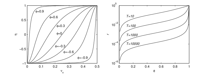
Figure 6: Correction of the periodogram of the quasistationary finite AR(1) process in comparison with the power spectrum of the stationary infinite AR(1) process.

The second factor in the correction (30) given by (31) is plotted in Fig. 6 for $\phi>0$ and a few values of $T$. It is a monotonic increasing function with respect to $\phi$ and

$$\lim_{\phi\rightarrow 1}r(\phi,T)=1~{}.$$ (34)

From (33) and (34) it follows that when $\phi\rightarrow 1$ the correction (30) is also approximately equal to $1$, so that the approximation (28) of the AR(1) power spectrum is wrong in the very dominant order. Reversely, for a given value of $\phi$, the relation (31) allows us to find the value of $T$ so that the correction $r$ should have the desired value.

If $T$ is even, then these conclusions hold for $\phi<0$ too, since $r$ changes only its sign $r(-\phi,T)=-r(\phi,T)$. But if $T$ is odd, then $\phi^{T}$ changes its sign and the function $r(\phi,T)$ acquires a different form. The most important modification is that, for $\phi\rightarrow-1$ the factor $r$ becomes infinite. Thus, in this case, the periodogram of the quasistationary finite AR(1) process is completely different from the power spectrum of the stationary infinite AR(1) process.

If the length $T$ is large enough such that the correction $\rho_{n}$ in (29) could be neglected, then the graphical representation of the finite AR(1) power spectrum is identical to that discussed in Section III. For example, when $T=1000$ and $\phi=0.9$ the correction (30) is $\rho_{n}=0.0095\,\eta(\phi,\nu_{n})<0.0095$ and it can be neglected. But for $T=1000$ and $\phi=0.99$ we have a much greater correction $\rho_{n}=0.0995\,\eta(\phi,\nu_{n})$. In Fig. 6 one can see that for $\phi$ near $1$, the factor $\eta$ is approximately $1$ excepting for very small frequencies. Therefore the correction $r$ is constant for almost all frequencies and the periodogram (29) differs from the spectral density (10) by the constant factor $1+\rho_{n}$. In log-log scale this constant factor shifts the periodogram parallel to the AR(1) power spectrum (see Fig. 7).

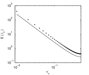
Figure 7: The periodogram of an finite AR(1) process with $T=100$ and $\phi=0.99$ (point markers) in comparison with the power spectrum of an infinite AR(1) process with the same $\phi$ (continuous line).

Because $\nu_{1}=0$, in a log-log scale the minimum frequency for a periodogram of a finite AR(1) process is $\nu_{2}=1/T$. Then the condition that the periodogram has a plateau can be obtained from (13)

$$T\gg\frac{2\pi\sqrt{\phi}}{1-\phi}~{}.$$ (35)

For example, when $\phi=0.99$ we have $T\gg 600$ and in Fig. 7 one can see that for $T=100$ the periodogram has no plateau.

V.2 The periodogram of the Brownian motion

The periodogram of the Brownian motion is obtained by replacing (21) and (22) in the formula resulting by averaging (26)

$$E\left\{I_{n}\right\} = \frac{\sigma^{2}}{2}\left(T+1\right)+\frac{\sigma^{2}}{2T}\sum_{\tau=1}^{T-1}\left(T-\tau\right)\left(T-\tau+1\right)$$ (36)

$$\left(\omega_{T}^{\tau\left(n-1\right)}+\omega_{T}^{-\tau\left(n-1\right)}\right).$$

After some calculations we obtain

$$E\left\{I_{n}\right\}=\frac{\sigma^{2}T}{8\sin^{2}\left(\frac{\pi}{T}\left(n-1\right)\right)}+\frac{\sigma^{2}\cos\left(\frac{2\pi}{T}\left(n-1\right)\right)}{2\sin^{2}\left(\frac{\pi}{T}\left(n-1\right)\right)}.$$ (37)

The dominant term in (37) is different from that in (29) for $\phi=1$ only by the factor $T/2.$ The relation (37) does not hold for $n=1$ because in the calculations we used relations incompatible with that special value. If in (36) we take $n=1$, then

$$E\left\{I_{1}\right\}=\frac{\sigma^{2}}{3}\left(T+1\right)\left(T^{2}-T+3\right).$$ (38)

In Fig. 8 we have plotted the dominant term of the periodogram (37) for $T=1000$. The most part of the graphic is a straight line since, if in (37) we consider $n\ll T$, then $E\left\{I_{n}\right\}\varpropto n^{-2}$. So in a log-log scale we obtain a straight line with the slope $-2$ and since the small frequencies region is strongly delated the most part of the graphic has this property. Figure 8 shows that outside of the plateau, the periodogram of the Brownian motion is parallel to the periodograms of quasistationary finite AR(1) processes with $\phi$ close to $1$ and the distance between them equals $\log(T/2)$ as shown above. This behavior is due to the fact that for $1-\phi\ll 1$ the value of the sine function at the denominator in (29) is dominant. Only for $\nu_{n}$ small enough the quantities (29) and (37) are significantly different.

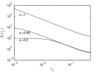
Figure 8: The periodogram of the Brownian motion in comparison with the periodograms of the quasistationary finite AR(1) process with $\phi=0.9$ and $0.99$.

VI Conclusions

Although the finite and infinite AR(1) processes are defined by the same recurrence relation, their properties can be very different when the serial correlation is large and the length of the finite AR(1) process is small. This difference is minimized if the first term of the finite AR(1) process is chosen such that its standard deviation should be equal to the standard deviation of the infinite AR(1) process. However, even in this case the periodogram of the finite AR(1) process for $\phi$ close to $\pm 1$ can significantly differ from the power spectrum of the infinite AR(1) process. That is why to numerically generate a time series as a realization of an AR(1) process we must take into account that the series length must be larger than the threshold value (35).

Although the AR(1) process is the simplest stochastic process describing the serial correlation only by means of a single parameter, it has remarkable properties which make it very useful as a first step in time series modeling. However, one has to take care that it is only one in the infinity of existing stochastic models and it is possible that an autoregressive structure to be incorrectly assigned to a time series. For example, although the autocovariance function (8) has an exponential decay, sometimes one attempted to model a $1/f$ noise characterized by a power law decay with autoregressive processes kau1999 , coza2003 . Therefore, it is necessary a thorough analysis of the AR(1) process properties not only in its infinite idealized form, but in the finite one as well. If the time series is not long enough, it is very likely that essential characteristics of the AR(1) process should be lost, as for example the existence of the plateau at small frequencies, and misinterpretations can occur.

- (1) G. E. P. Box and G. M. Jenkins, Time Series Analysis: Forcasting and Control, 2nd ed. (Holden-Day, San Francisco, 1976).
- (2) S. Hallerberg, E. G. Altmann, D. Holstein, and H. Kantz, Phys. Rev. E 75, 016706 (2007).
- (3) J. Gao, J. Hu, W. Tung, Y. Cao, N. Sarshar, V.P. Roychowdhury, Phys. Rev. E 73, 016117 (2006).
- (4) D. Maraun, H.W. Rust, J. Timmer, Nonlinear Processes in Geophysics 11, 495-503 (2004).
- (5) D. T. Liley, P. J. Cadusch, M. Gray, and P. J. Nathan, Phys. Rev. E 68, 051906 (2003).
- (6) L. Guzman-Vargas and F. Angulo-Brown, Phys. Rev. E 67, 052901 (2003).
- (7) A. Király and I. M. Jánosi, Phys. Rev. E 65, 051102 (2002).
- (8) J. Timmer, U. Schwarz, H.U. Voss, I. Wardinski, T. Belloni, G. Hasinger, M. van der Klis, J. Kurths, Phys. Rev. E 61, 1342 (2000).
- (9) M. Palus, D. Novotna, Phys. Rev. Lett. 83, 3406 (1999).
- (10) C. Vamoş, Phys. Rev. E 75, 036705 (2007).
- (11) D. Kugiumtzis, Phys. Rev. E 66, 025201 (2002).
- (12) R. Blender, Phys. Rev. E 64, 067101 (2001).
- (13) P.J. Brockwell and R. Davis, Time Series: Theory and Methods, (Springer-Verlag, New York, 1991).
- (14) P.J. Brockwell and R. Davis, Introduction to Time Series and Forecasting, (Springer-Verlag, New York, 1996).
- (15) J.D. Hamilton, Time Series Analysis, (Princeton University Press, 1994).
- (16) P. Stoica and R. L. Moses, Introduction to Spectral Analysis (Prentice-Hall, New Jersey, 1997).
- (17) B. Kaulakys, Physics Letters A 257, 37 (1999).
- (18) A. Coza, V.V. Morariu, Physica A 320, 449 (2003).