Quantum Entanglement Capacity with Classical Feedback

Abstract

For any quantum discrete memoryless channel, we define a quantity called quantum entanglement capacity with classical feedback ($E_{B}$), and we show that this quantity lies between two other well-studied quantities. These two quantities - namely the quantum capacity assisted by two-way classical communication ($Q_{2}$) and the quantum capacity with classical feedback ($Q_{B}$) - are widely conjectured to be different: there exists quantum discrete memoryless channel for which $Q_{2}>Q_{B}$. We then present a general scheme to convert any quantum error-correcting codes into adaptive protocols for this newly-defined quantity of the quantum depolarizing channel, and illustrate with Cat (repetition) code and Shor code. We contrast the present notion with entanglement purification protocols by showing that whilst the Leung-Shor protocol can be applied directly, recurrence methods need to be supplemented with other techniques but at the same time offer a way to improve the aforementioned Cat code. For the quantum depolarizing channel, we prove a formula that gives lower bounds on the quantum capacity with classical feedback from any $E_{B}$ protocols. We then apply this formula to the $E_{B}$ protocols that we discuss to obtain new lower bounds on the quantum capacity with classical feedback of the quantum depolarizing channel.

I Introduction

Quantum information theoryN7 ; B5 studies transmission and manipulation of information in systems that must be treated quantum mechanically, and it is markedly different from classical information theoryB2 ; N8 in which the capacity of a classical discrete memoryless channel is uniquely given by a single numerical value representing the amount of information that can be transmitted asymptotically without error per channel use. Moreover, this value is unaffected by the use of classical feedback. However, for quantum discrete memoryless channels, capacities are affected by side classical communication and shared entanglements1 ; 6 ; 7 . In addition, we can use a quantum channel to transmit either classical or quantum information and therefore we can define, for every quantum discrete memoryless channel, various capacities: $C$, unassisted classical capacity; $C_{B}$, classical capacity assisted by classical feedback; $C_{2}$, classical capacity assisted by independent classical information; $C_{E}$, entanglement-assisted classical capacity; $Q$, unassisted quantum capacity; $Q_{B}$, quantum capacity assisted by classical feedback; $Q_{2}$, quantum capacity assisted by independent classical information; and finally $Q_{E}$, entanglement-assisted quantum capacity.

So far, some progress has been made to compute the capacities for specific channels17 ; 6 ; 13 . However, search for a general formula only succeeded in a few cases7 ; 39 ; 2 ; 3 ; 8 , and progress in this direction has been hindered by the additivity conjecture28 ; 29 ; 41 ; 9 . While we are far from obtaining a formula for all these capacities, a natural question to ask is whether we can relate these capacities. Some relations such as $C\geq Q$ are trivial but others can be hard. Some capacities are even incomparable, i.e. depending on the channel, either one may be greater than the other. For the comparable capacities, we also want to show whether the inequalities are strict or saturable. Our present knowledge of these relations is summarized in 1 ; 5 .

One of the conjectural relations is $Q_{2}>Q_{B}$, that there exist quantum channels whose quantum capacity assisted by two-way classical communication exceeds their quantum capacity assisted by classical feedback. While we cannot prove the conjecture, the aim of this work is to define, for any quantum discrete memoryless channel, a quantity called quantum entanglement capacity with classical feedback ($E_{B}$). We show that this capacity lies between $Q_{B}$ and $Q_{2}$, and it has two different well-defined operational meanings. For the quantum depolarizing channel, we demonstrate a general scheme to convert quantum error-correcting codes (QECC) into $E_{B}$ protocols, and these in turn imply new lower bounds on the quantum capacity with classical feedback ($Q_{B}$).

This work is also closely related to entanglement purification protocols (EPP)35 ; N18 ; LS1 ; 51 ; N17 , procedures by which two parties can extract pure-state entanglement out of some shared mixed entangled states. For example,

$$00: \ket{\Phi^{+}}=\frac{1}{\sqrt{2}}(\ket{\uparrow\uparrow}+\ket{\downarrow\downarrow})$$

$$01: \ket{\Psi^{+}}=\frac{1}{\sqrt{2}}(\ket{\uparrow\downarrow}+\ket{\downarrow\uparrow})$$

$$10: \ket{\Phi^{-}}=\frac{1}{\sqrt{2}}(\ket{\uparrow\uparrow}-\ket{\downarrow\downarrow})$$

$$11: \ket{\Psi^{-}}=\frac{1}{\sqrt{2}}(\ket{\uparrow\downarrow}-\ket{\downarrow\uparrow})$$ (1)

are the so-called Bell basis and each of these states is considered equivalent to an ebit, a basic unit of entanglement in quantum information theory. At the beginning of these entanglement purification protocols, two persons Alice and Bob share a large number of the generalized Werner statesN14

$$\rho_{F}=F\ket{\Phi^{+}}\bra{\Phi^{+}}+\frac{1-F}{3}\big{(}\ket{\Phi^{-}}\bra{\Phi^{-}}+\ket{\Psi^{+}}\bra{\Psi^{+}}+\ket{\Psi^{-}}\bra{\Psi^{-}}\big{)},$$ (2)

say $\rho_{F}^{\otimes N}$, and they are allowed to communicate classically, apply unitary transformations and perform projective measurements. In the end the quantum states $\Upsilon$ shared by Alice and Bob are to be a close approximation of the maximally entangled states $(\ket{\Phi^{+}}\bra{\Phi^{+}})^{\otimes M}$, or more precisely we require the fidelity between $\Upsilon$ and $(\ket{\Phi^{+}}\bra{\Phi^{+}})^{\otimes M}$ approaches one as $N$ goes to infinity. We then define the yield of such protocols to be $M/N$. Entanglement purification protocols (EPP) are further divided into 1-EPP and 2-EPP according to whether the sender and receiver are allowed to communicate uni- or bi-directionally.

One of the main reasons why this is considered general is the equivalence between an entanglement purification protocol on the Werner state $\rho_{F}$ and a protocol to faithfully transmit quantum states through the $\frac{(4F-1)}{3}$-depolarizing channel established in 35 . A $p$-depolarizing channel is a simple qubit channel such that a qubit passes through the channel undisturbed with probability $p$ and outputs as a completely random qubit with probability $1-p$. Specifically, the yield of a 1-EPP on the Werner state $\rho_{F}$ is equal to the unassisted quantum capacity of a $\frac{(4F-1)}{3}$-depolarizing channel ($Q$); and the yield of a 2-EPP on the Werner state $\rho_{F}$ is equal to the quantum capacity assisted by two-way classical communication of a $\frac{(4F-1)}{3}$-depolarizing channel ($Q_{2}$). The equivalence was proved by noting that the EPR pair $\ket{\Phi^{+}}$ becomes the Werner state $\rho_{F}$ if Alice passes the second half through the $\frac{(4F-1)}{3}$-depolarizing channel. The present study of the amount of entanglements Alice and Bob can share by using the depolarizing channel and classical feedback is clearly related, and we will exploit the similarities and differences to obtain new results and ask new questions.

I.1 Structure of the paper

In section I.2, we review some previous entanglement purification protocols that will be used in this paper. In section II, we define a new quantity called quantum entanglement capacity with classical feedback ($E_{B}$) and this quantity is shown to lie between $Q_{B}$ and $Q_{2}$. We will then give an alternate operational meaning of $E_{B}$. In section III, we describe how one can turn a QECC into an $E_{B}$ protocol and illustrate the idea with Cat (repetition) code and Shor code. We then connect the present notion to the modified recurrence method and Leung-Shor method. In section IV, we compute new lower bounds on $Q_{B}$ implied by these $E_{B}$ protocols. Finally, we conclude with a characteristic of the threshold of Cat code and other further research directions.

I.2 Previous works

I.2.1 Universal hashing

Universal hashing, introduced in 35 , requires only one-way classical communication and hence is a 1-EPP. The hashing method works by having Alice and Bob each perform some local unitary operations on the corresponding members of the shared bipartite quantum states. They then locally measure some of the pairs to gain classical information about the identities of the the remaining unmeasured pairs. It was shown that each measurement can be made to reveal almost 1 bit of information about the unmeasured Bell states pairs. Since the information associated with a quantum state $\rho_{F}$ is given by its von Neumann entropy $S(\rho_{F})$, we know from typical subspace argument that, with probability approaching 1 and by measuring $NS(\rho_{F})$ pairs, Alice and Bob can figure out the identities of all pairs including the unmeasured ones. Once the identities of the Bell states are known, Alice and Bob can convert them into the standard states $\Phi^{+}$ easily. Therefore this protocol distills a yield of $\Big{(}N-NS(\rho_{F})\Big{)}/N=1-S(\rho_{F})$.

I.2.2 The recurrence method and the modified recurrence method

Figure 1: The recurrence method.

The recurrence methodN12 ; 35 is illustrated in figure 1. Alice and Bob put the quantum states $\rho_{F}^{\otimes N}$ into groups of two and apply XOR operations to the corresponding members of the quantum states $\rho_{F}^{\otimes 2}$, one as the source and one as the target. They then take projective measurements on the target states along the z-axis, and compare their measurement results with the side classical communication channel. If they get identical results, the source pair “passed”; otherwise the source pair “failed”. Alice and Bob then collect all the “passed” pairs, and iterate this process until it becomes more beneficial to pass on to the universal hashing. If we denote the quantum states by $\rho=p_{00}\ket{\Phi^{+}}\bra{\Phi^{+}}+p_{01}\ket{\Psi^{+}}\bra{\Psi^{+}}+p_{10}\ket{\Phi^{-}}\bra{\Phi^{-}}+p_{11}\ket{\Psi^{-}}\bra{\Psi^{-}}$, then this protocol has the following recurrence relation:

$$p^{\prime}_{00}=(p_{00}^{2}+p_{10}^{2})/p_{pass}; p^{\prime}_{01}=(p_{01}^{2}+p_{11}^{2})/p_{pass};$$ (3)

$$p^{\prime}_{10}=2p_{01}p_{11}/p_{pass}; p^{\prime}_{11}=2p_{00}p_{10}/p_{pass};$$

and

$$p_{pass}=p_{00}^{2}+p_{01}^{2}+p_{10}^{2}+p_{11}^{2}+2p_{00}p_{10}+2p_{01}p_{11}.$$ (4)

This is known as the recurrence method. As mentioned in 35 , C. Macchiavello has found that if we apply a unilateral $\pi$ rotation $\sigma_{x}$ followed by a bilateral $\pi/2$ rotation $B_{x}$, faster convergence is achieved and this is known as the modified recurrence method. Computationally, one has to switch the $p_{10}$ and $p_{11}$ components after each recurrence.

I.2.3 The Leung-Shor method

Figure 2: The Leung-Shor method.

The Leung-Shor methodLS1 is illustrated in figure 2. Alice and Bob share the quantum states $\rho_{F}^{\otimes N}$ and put them into groups of four. They then apply the quantum circuit shown in figure 2 and take measurements on the third and fourth pairs along the x- and z-axis respectively. Using the side classical communication channel, they can compare their results with each other. If they get identical results on both measurements, they keep the first and second pairs and apply universal hashing35 . If either of the two results disagrees, they throw away all four pairs.

The four pairs can be described by an 8-bit binary string as in (1), and since these are mixed states they are in fact probability distribution over all $256(=2^{8})$ possible 8-bit binary strings. The quantum circuit consists only of XOR gates and therefore maps the 8-bit binary strings, along with their underlying probability distribution, bijectively to themselves. If we let the probability distributions before and after the quantum gates to be $P(a_{1}a_{2}b_{1}b_{2}c_{1}c_{2}d_{1}d_{2})$ and $P^{\prime}(a_{1}a_{2}b_{1}b_{2}c_{1}c_{2}d_{1}d_{2})$ respectively, then the yield of this method is:

$$\frac{p_{pass}}{2}\bigg{(}1-\frac{H(Q(a_{1}a_{2}b_{1}b_{2}))}{2}\bigg{)}$$ (5)

where $p_{pass}=\sum_{a_{1},a_{2},b_{1},b_{2},c_{2},d_{1}\in\{0,1\}}P^{\prime}(a_{1}a_{2}b_{1}b_{2}0c_{2}d_{1}0)$ is the “pass” probability, $Q(a_{1}a_{2}b_{1}b_{2})=\sum_{c_{2},d_{1}\in\{0,1\}}P^{\prime}(a_{1}a_{2}b_{1}b_{2}0c_{2}d_{1}0)/p_{pass}$ is the post-measurement probability distribution and $H(Q(a_{1}a_{2}b_{1}b_{2}))$ is the Shannon entropy function.

II A quantity that lies between $Q_{B}$ and $Q_{2}$

In this section, we define, for any quantum discrete memoryless channel, a quantity called quantum entanglement capacity with classical feedback $E_{B}$. We will show that this quantity is less than the quantum capacity with two-way classical communication $Q_{2}$ and is greater than the quantum capacity with classical feedback $Q_{B}$.

II.1 Definition of $E_{B}$

Quantum entanglement capacity with classical feedback of a QDMC can be loosely described as the maximal asymptotic rate at which the sender Alice can share the entangled state $\ket{\Phi^{+}}\in\mathcal{H}_{2}^{\otimes 2}$ with the receiver Bob with the assistance of a classical feedback channel. Precisely, let the QDMC be described by

$$\mathcal{N}:\mathcal{B}(\mathcal{H}_{d_{1}})\longrightarrow\mathcal{B}(\mathcal{H}_{d_{2}})$$

$$\rho\mapsto\rho^{\prime}=\sum_{i}E_{i}\rho E_{i}^{\dagger},$$

where $\sum_{j}E_{j}^{\dagger}E_{j}=I$ and $\{E_{i}\}$ is a set of linear operators which map the input Hilbert space $\mathcal{H}_{d_{1}}$ to the output Hilbert space $\mathcal{H}_{d_{2}}$. Then in the first round of any $E_{B}$ protocols, Alice prepares a quantum state $\alpha_{1}=\ket{\Upsilon}\bra{\Upsilon}\in\mathcal{B}(\mathcal{H}_{d_{1}}^{\otimes N}\otimes\mathcal{H}_{a})$, where $\mathcal{H}_{a}$ is the Hilbert space representing the ancilla system in her laboratory and she sends the first part of the quantum state to Bob via the quantum channel $\mathcal{N}$:

$$\mathcal{N}:\mathcal{B}(\mathcal{H}_{d_{1}}) \longrightarrow \mathcal{B}(\mathcal{H}_{d_{2}})$$

$$\rho_{1}=tr_{(d_{1}^{N-1}\times a)}(\ket{\Upsilon}\bra{\Upsilon}) \mapsto \rho_{1}^{\prime}=\sum_{i}E_{i}\rho_{1}E_{i}^{\dagger}.$$

After sending $\rho_{1}$, Alice’s quantum system is described by $\alpha_{1}^{\prime}=tr_{d_{1}}(\alpha_{1})\in\mathcal{B}(\mathcal{H}_{d_{1}}^{\otimes(N-1)}\otimes\mathcal{H}_{a})$. On the other hand, Bob is now in possession of the quantum state $\rho_{1}^{\prime}$ he just received from Alice as well as the ancilla system in his laboratory, and therefore his quantum system can be described by $\beta_{1}^{\prime}=\rho_{1}^{\prime}\otimes\beta_{1}=\rho_{1}^{\prime}\otimes\ket{0}\bra{0}^{\otimes\log_{2}b}\in\mathcal{B}(\mathcal{H}_{d_{2}}\otimes\mathcal{H}_{b})$. Next Bob performs local quantum operation on his quantum system:

$$\mathbf{B}:\mathcal{B}(\mathcal{H}_{d_{2}}\otimes\mathcal{H}_{b}) \longrightarrow \mathcal{B}(\mathcal{H}_{d_{2}}\otimes\mathcal{H}_{b})$$

$$\beta_{1}^{\prime} \mapsto \beta_{1}^{\prime\prime}=\sum_{i}B_{i}\beta_{1}^{\prime}B_{i}^{\dagger}$$

where $\sum_{i}B_{i}^{\dagger}B_{i}=I$. Bob then uses the feedback channel to send classical information to Alice. Note that if Bob’s operation comprised quantum measurements, this classical information could include the measurement results$(i)$. Upon learning the classical information sent by Bob, Alice’s quantum system transforms from $\alpha_{1}^{\prime}$ to $\alpha_{1,(i)}^{\prime}$ and she performs operation on her quantum system:

$$\mathbf{A_{(i)}}:\mathcal{B}(\mathcal{H}_{d_{1}}^{\otimes(N-1)}\otimes\mathcal{H}_{a}) \longrightarrow \mathcal{B}(\mathcal{H}_{d_{1}}^{\otimes(N-1)}\otimes\mathcal{H}_{a})$$

$$\alpha_{1,(i)}^{\prime} \mapsto \alpha_{1,(i)}^{\prime\prime}=\sum_{j}A_{j,(i)}\alpha_{1,(i)}^{\prime}A_{j,(i)}^{\dagger}.$$

Note that both the quantum system $\alpha_{1,(i)}^{\prime}$ and Alice’s operation $\mathbf{A_{(i)}}$ are dependent on the classical information(i) she received from Bob. This is the end of the first round of any general $E_{B}$ protocols and can be summarized as:

$$\mathbf{LOCC_{A\leftarrow B}}^{(1)}\circ\mathbf{N}^{(1)}:\mathcal{B}(\mathcal{H}_{d_{1}}^{\otimes N}\otimes\mathcal{H}_{a}\otimes\mathcal{H}_{b}) \longrightarrow \mathcal{B}(\mathcal{H}_{d_{1}}^{\otimes(N-1)}\otimes\mathcal{H}_{a}\otimes\mathcal{H}_{d_{2}}\otimes\mathcal{H}_{b})$$

$$\omega_{1} \mapsto \omega_{2}.$$

The second round of the protocols starts with Alice holding $\alpha_{2}=tr_{(d_{2}\times b)}(\omega_{2})$ and Bob holding $\beta_{2}=tr_{(d_{1}^{N-1}\times a)}(\omega_{2})$. After $N$ rounds of protocols as seen in figure 3, we require the fidelity between the quantum state shared between Alice and Bob, $\omega_{N+1}$, and the quantum state, $(\ket{\Phi^{+}}\bra{\Phi^{+}})^{\otimes M}$, to approach 1 as $N$ goes to infinity. Then we define $E_{B}(\mathcal{N})$ to be the supremum of any attainable $\frac{M}{N\log_{2}(d_{2})}$ - or simply $M/N$ if $d_{2}=2$.

Note that in this work, when we discuss an $E_{B}$ protocol, for brevity, we often say to compute the $E_{B}$ associated with the protocol rather than to compute the lower bounds on $E_{B}(\mathcal{N})$ impled by the protocol.

Figure 3: An $E_{B}$ protocols for channel $\mathcal{N}$(See the text for details).

II.2 $E_{B}\leq Q_{2}$

To show $E_{B}\leq Q_{2}$, we simply convert any $E_{B}$ protocol to a $Q_{2}$ protocol with the same rate. Suppose we have a protocol on $\mathcal{N}$ and this $E_{B}(\mathcal{N})$ protocol achieves $\frac{M}{N\log_{2}(d_{2})}$, then at the end of this protocol Alice and Bob share the quantum state $\ket{\Phi^{+}}\bra{\Phi^{+}}^{\otimes M}$. Alice now uses the forward classical communication channel to teleport any quantum state $\rho\in\mathcal{H}_{2}^{\otimes M}$ and therefore this new $Q_{2}(\mathcal{N})$ protocol achieves $\frac{M}{N\log_{2}(d_{2})}$.

II.3 $Q_{B}\leq E_{B}$

This follows from the fact that $Q_{B}$ protocols are more restricted than $E_{B}$ protocols because in defining quantum capacities12 the sender is required to not only transmit the quantum state $\rho$ but also preserve its entanglement with the environment to which neither the sender nor the receiver has access. In $E_{B}$ protocols, the sender is required to transmit half of the maximally entangled states $\ket{\Phi^{+}}^{M}$ and is in possession of the other half which she can manipulate in her laboratory. Concisely, one can convert any $Q_{B}$ protocol to an $E_{B}$ protocol as follows: Alice prepares $\ket{\Phi^{+}}\bra{\Phi^{+}}^{\otimes M}\in\mathcal{B}(\mathcal{H}_{2}^{\otimes M}\otimes\mathcal{H}_{2}^{\otimes M})$ in her laboratory and performs the $Q_{B}$ protocol on $\rho=(I/2)^{\otimes M}=tr_{(2^{M})}(\ket{\Phi^{+}}\bra{\Phi^{+}}^{\otimes M})$. At the end of the protocol, Alice and Bob share the bipartite quantum state $\ket{\Phi^{+}}\bra{\Phi^{+}}^{\otimes M}$ and hence $E_{B}(\mathcal{N})\geq Q_{B}(\mathcal{N})\geq\frac{M}{N\log_{2}(d_{2})}$.

II.4 $E_{B}$ as quantum backward capacity with classical feedback

In section II.1, $E_{B}$ was defined as the maximal asymptotic rate at which Alice shares the singlet state $\ket{\Phi^{+}}$ with Bob with the assistance of a classical feedback channel. Alternatively, we can associate $E_{B}$ with a different operational meaning, namely the asymptotic rate at which Bob can send quantum states to Alice. This is because after any $E_{B}$ protocols Alice and Bob share the quantum states $(\ket{\Phi^{+}}\bra{\Phi^{+}})^{M}$ and there is a classical channel from Bob to Alice. Therefore, Bob can teleport any quantum states $\rho\in\mathcal{H}_{2}^{\otimes M}$ to Alice and this achieves the same yield $\frac{M}{N\log_{2}(d_{2})}$ if we normalize by the dimension of the output Hilbert space or if we assume the input Hilbert space and the output Hilbert space are of the same size. Trivially, if Bob can send quantum states to Alice, Bob can choose to send half of the EPR pair $\ket{\Phi^{+}}$. Therefore these two notions are equivalent to one another.

III Adaptive quantum error-correcting codes (AQECC)

In quantum error-correcting codesN21 ; B5 ; N19 ; N20 , quantum states are encoded into the subspace of some larger Hilbert space. Although it has been discovered that quantum states can more generally be encoded into a subsystem rather than a subspaceN23 ; N22 , we focus only on subspace encoding. Our aim is to convert any quantum error-correcting codes (QECC) to new adaptive $E_{B}$ protocols on the quantum depolarizing channel $\mathcal{E}_{p}$. In section III.1, we briefly review the stabilizer formalism; and in section III.2 we introduce the idea of AQECC. In the rest of the section, we will illustrate with and compute the $E_{B}(\mathcal{E}_{p})$ for two QECC, namely the Cat code and Shor code. We then consider how the recurrence methods - a 2-EPP - in I.2.2 can be turned into an $E_{B}$ protocol. Finally we explain that the Leung-Shor method35 in I.2.3 is in fact an $E_{B}$ protocol.

III.1 Stabilizer formalism for QECC

We will briefly review stabilizer formalism and introduce some notations. A clear and detailed discussion can be found in B5 . $G_{n}$ denotes the Pauli group on $n$ qubits, and therefore consists of the n-fold tensor products of Pauli matrices. For example,

$$G_{1}=\{\pm I,\pm iI,\pm X,\pm iX,\pm Y,\pm iY,\pm Z,\pm iZ\}$$

where $X=\sigma_{x}$, $Y=\sigma_{y}$ and $Z=\sigma_{z}$. We use subscripts to denote the qubit that a Pauli matrix acts on. For example, $X_{2}Y_{4}$ means $I\otimes X\otimes I\otimes Y\otimes I\otimes\ldots\otimes I\in G_{n}$. Generators of a subgroup $S\subset G_{n}$ are independent if for any $i=1,2,3,\dots,n-k$,

$$<g_{1},\dots,g_{i-1},g_{i+1},\ldots,g_{n-k}>\neq<g_{1},\dots,g_{n-k}>.$$

We say a vector space $V_{S}\subset\mathcal{H}_{2}^{\otimes n}$ is stabilized by a subgroup $S\subset G_{n}$ if for any $\ket{\phi}\in V_{S}$ and for any $s\in S$,

$$s\ket{\phi}=\ket{\phi}.$$

The following lemma can be shown easily:

Lemma 1

Let $S=<g_{1},\ldots,g_{n-k}>$ be generated by $n-k$ independent and commuting elements from $G_{n}$, and $-I\not\in S$. Then $V_{S}$ is a $2^{k}$-dimensional vector space.

Therefore to specify a $2^{k}$-dimensional subspace for error-correcting codes, we only need to specify $n-k$ independent generators $g_{1},\ldots,g_{n-k}$. However we still need to specify the logical basis vectors $\ket{x_{1},\ldots,x_{k}}_{L}$ within $V_{S}$. In this work, we only deal with codes where $k=1$. Therefore, it suffices to specify the logical $\bar{X}$ and logical $\bar{Z}$ such that $\bar{X}\ket{0}_{L}=\ket{1}_{L}\in\mathcal{H}_{2}^{\otimes n}$, $\bar{X}\ket{1}_{L}=\ket{0}_{L}\in\mathcal{H}_{2}^{\otimes n}$, $\bar{Z}\ket{0}_{L}=\ket{0}_{L}\in\mathcal{H}_{2}^{\otimes n}$ and $\bar{Z}\ket{1}_{L}=-\ket{1}_{L}\in\mathcal{H}_{2}^{\otimes n}$. Note that in doing so, we indirectly specify $\ket{0}_{L}$ and $\ket{1}_{L}$.

III.2 $E_{B}$ protocols via AQECC

Recall the aim of any $E_{B}$ protocols is for Alice to share the bipartite state $\ket{\Phi^{+}}=\frac{1}{\sqrt{2}}(\ket{00}+\ket{11})$ with Bob. We will explain our idea of turning a QECC to an $E_{B}$ protocol in two steps.

The first step is to simply encode half of the EPR pair $\ket{\Phi^{+}}$ in an $[n,1]$ stabilizer code, one that encodes a qubit in an $2^{n}$-dimensional Hilbert space $\mathcal{H}_{2}^{\otimes n}$. Alice performs the encoding

$$\mathbf{A}:\mathcal{B}(\mathcal{H}_{2})\longrightarrow\mathcal{B}(\mathcal{H}_{2}^{\otimes n})$$

$$tr_{2}(\ket{\Phi^{+}}\bra{\Phi^{+}})\mapsto\alpha_{1}$$

and then sends the $n$ qubits through the $p$-depolarizing channel

$$\mathcal{E}_{p}:\mathcal{B}(\mathcal{H}_{2}) \longrightarrow \mathcal{B}(\mathcal{H}_{2})$$

$$\rho \mapsto \frac{1+3p}{4}\times\rho+\frac{1-p}{4}\times(\sigma_{x}\rho\sigma_{x}^{\dagger}+\sigma_{y}\rho\sigma_{y}^{\dagger}+\sigma_{z}\rho\sigma_{z}^{\dagger}).$$

Since the error elements of the $p$-depolarizing channel are Pauli matrices, Alice can choose the logical basis states (or alternatively the logical operators $\bar{X},\bar{Z}$ as we explained in the previous section) in such a way that after the error-correction operation $\mathbf{B}$, the encoded qubit has either an $X$ error, a $Y$ error, a $Z$ error or no error. Since $X\ket{\Phi^{+}}=\ket{\Psi^{+}}$, $Y\ket{\Phi^{+}}=\ket{\Psi^{-}}$ and $Z\ket{\Phi^{+}}=\ket{\Phi^{-}}$, the bipartite state between Alice and Bob will be a probabilistic mixture of the four Bell states. Therefore Bob can use the classical feedback channel to perform universal hashing and distill perfect EPR pairs $\ket{\Phi^{+}}=\frac{1}{\sqrt{2}}(\ket{00}+\ket{11})$. This first step is illustrated in figure 4.

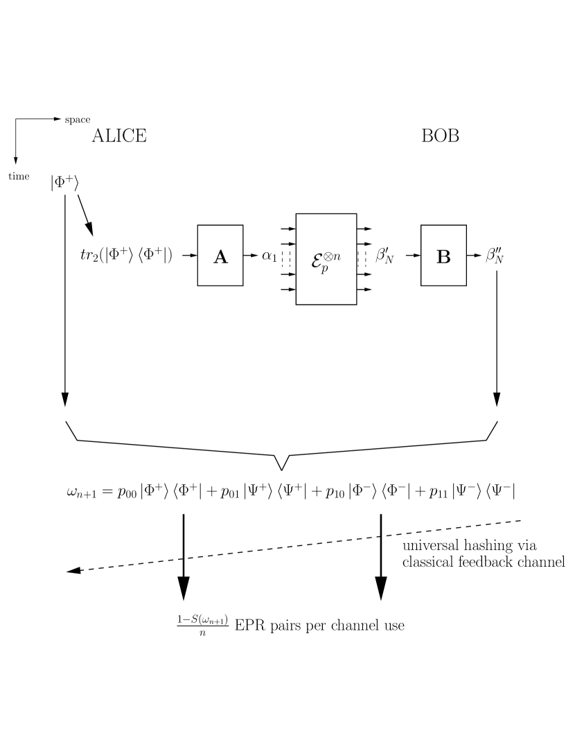
Figure 4: Encoding half of the EPR pair $\ket{\Phi^{+}}$ with a QECC .

The second step is to modify what has just been described so as to achieve a higher rate. Recall an $[n,1]$ stabilizer code is described by the generators of a subgroup $S=<g_{1},g_{2},\ldots,g_{n-2},g_{n-1}>$. The error-correcting operation $\mathbf{B}$ performed by Bob involves measuring the observables $g_{1},g_{2},\ldots,g_{n-1}$ since they are all tenser products of Pauli matrices acting on n qubits. Note that, however, many of the $g_{i}$’s have identity action on all but a few qubits. For example, in 9-bit Shor code, $g_{1}=Z_{1}Z_{2}$($=Z_{1}\otimes Z_{2}\otimes I_{3}\otimes I_{4}\otimes I_{5}\otimes I_{6}\otimes I_{7}\otimes I_{8}\otimes I_{9}$). Also, whenever a measurement result ‘-1’ is obtained, it means some errors have occurred. In the case of Shor code, if Bob takes a measurement on the first two qubits immediately after he receives them from Alice and the measurement result is ‘-1’, it is better for Bob to use the classical feedback channel to inform Alice that some errors have occurred in the first 2 qubits and they should give up this block of transmission and start all over. It is because the quantum state $\omega_{n+1}$ Alice and Bob obtained after n channel uses and decoding will be more mixed - or in other words of higher entropy - if some errors have occurred. It is thus more economical to not continue with this particular block of codes and give up the few qubits that have already been transmitted.

It is thus important to arrange the order of the measurements $g_{1},g_{2},\ldots,g_{n-1}$ such that it only involves as few more qubits as possible when one goes down the list. So that when an error is detected early on, Alice and Bob can stop the block and start all over so as to save more channel uses. For example, the generators of Shor code can be arranged as follows:

$$g_{1} = Z_{1}\otimes Z_{2}\otimes I_{3}\otimes I_{4}\otimes I_{5}\otimes I_{6}\otimes I_{7}\otimes I_{8}\otimes I_{9}$$

$$g_{2} = I_{1}\otimes Z_{2}\otimes Z_{3}\otimes I_{4}\otimes I_{5}\otimes I_{6}\otimes I_{7}\otimes I_{8}\otimes I_{9}$$

$$g_{3} = I_{1}\otimes I_{2}\otimes I_{3}\otimes Z_{4}\otimes Z_{5}\otimes I_{6}\otimes I_{7}\otimes I_{8}\otimes I_{9}$$

$$g_{4} = I_{1}\otimes I_{2}\otimes I_{3}\otimes I_{4}\otimes Z_{5}\otimes Z_{6}\otimes I_{7}\otimes I_{8}\otimes I_{9}$$

$$g_{5} = X_{1}\otimes X_{2}\otimes X_{3}\otimes X_{4}\otimes X_{5}\otimes X_{6}\otimes I_{7}\otimes I_{8}\otimes I_{9}$$

$$g_{6} = I_{1}\otimes I_{2}\otimes I_{3}\otimes I_{4}\otimes I_{5}\otimes I_{6}\otimes Z_{7}\otimes Z_{8}\otimes I_{9}$$

$$g_{7} = I_{1}\otimes I_{2}\otimes I_{3}\otimes I_{4}\otimes I_{5}\otimes I_{6}\otimes I_{7}\otimes Z_{8}\otimes Z_{9}$$

$$g_{8} = I_{1}\otimes I_{2}\otimes I_{3}\otimes X_{4}\otimes X_{5}\otimes X_{6}\otimes X_{7}\otimes X_{8}\otimes X_{9}$$ (6)

It is conceivable that after a large portion of the qubits in a block have been transmitted, it is better to continue even if an error is detected. It is indeed the case for Shor code when the probability parameter $p$ of the channel $\mathcal{E}_{p}$ is large. In the next two sections, we will apply this AQECC idea to Cat code and Shor code, and compute the lower bounds on $E_{B}(\mathcal{E}_{p})$ implied by these codes.

III.3 Cat code and modified Cat code

The n-bit Cat (repetition) code is an $[n,1]$ stabilizer code with the following generators

$$g_{1} = Z_{1}Z_{2}$$

$$g_{2} = Z_{2}Z_{3}$$

$$g_{3} = Z_{3}Z_{4}$$

$$\vdots \vdots \vdots$$

$$g_{n-2} = Z_{n-2}Z_{n-1}$$

$$g_{n-1} = Z_{n-1}Z_{n}$$

and we choose the following logical operators

$$\bar{X} = X_{1}X_{2}\ldots X_{n-1}X_{n}$$

$$\bar{Z} = Z_{1}Z_{2}\ldots Z_{n-1}Z_{n}\textrm{ if n is odd and }$$

$$\bar{Z} = Z_{1}Z_{2}\ldots Z_{n-1}I_{n}\textrm{ if n is even.}$$

This in turn determines the logical computational basis

$$\ket{0}_{L}=\ket{00\ldots 00}\in\mathcal{H}_{2}^{\otimes n}\textrm{ and }\ket{1}_{L}=\ket{11\ldots 11}\in\mathcal{H}_{2}^{\otimes n}.$$

Therefore, the singlet state $\frac{1}{\sqrt{2}}(\ket{00}+\ket{11})\in\mathcal{H}_{2}^{\otimes 2}$ is encoded as $\frac{1}{\sqrt{2}}(\ket{00\ldots 00}+\ket{11\ldots 11})\in\mathcal{H}_{2}^{\otimes n+1}$ in Alice’s laboratory. Alice will send the last n qubits to Bob via the channel $\mathcal{E}_{p}$. In accordance with the AQECC idea in the previous section, Alice sends the first two qubits first and Bob takes the measurement $g_{1}$. If the measurement result is ‘-1’, Bob will inform Alice of the result via the classical feedback channel and Alice will discard the n-1 qubits remaining in her laboratory and start all over by encoding another EPR pair and sending the quantum states. If the measurement result is ‘+1’, Bob will inform Alice of the result and Alice will continue to send the third qubit. Bob will then measure $g_{2}$. This continues until all n qubits are passed to Bob and Bob gets ‘+1’ in all n-1 measurements $g_{1},g_{2},\ldots,g_{n-1}$. Alice and Bob will then process a bipartite quantum state $\omega_{n+1}\equiv p_{00}\ket{\Phi^{+}}\bra{\Phi^{+}}+p_{01}\ket{\Psi^{+}}\bra{\Psi^{+}}+p_{10}\ket{\Phi^{-}}\bra{\Phi^{-}}+p_{11}\ket{\Psi^{-}}\bra{\Psi^{-}}$ that is Bell diagonal. If Alice and Bob repeat the process until they share N copies of $\omega_{n+1}$, i.e. $\omega_{n+1}^{\otimes N}$, they can perform universal hashing on these states and they will have $N\Big{(}1-H(p_{00},p_{01},p_{10},p_{11})\Big{)}$ EPR pairs $\ket{\Phi^{+}}$. However we are interested in the yield per channel use. Let $p_{i}=\textrm{prob}(\textrm{`+1' for measurement }g_{i})$. Then the average number of channel uses needed before we successfully pass a block of n-qubit Cat code through the depolarizing channel is given by

$$n^{*} = \bigg{(}\sum_{i=2}^{n-1}\Big{(}i\times(\prod_{j=1}^{i-2}p_{j})\times(1-p_{i-1})\Big{)}+n\times\prod_{i=1}^{n-2}p_{i}\bigg{)}/\bigg{(}n\times\prod_{i=1}^{n-1}p_{i}\bigg{)}$$

$$= \bigg{(}2\times(1-p_{1})+3\times p_{1}\times(1-p_{2})+\ldots+(n-1)\times p_{1}\times p_{2}\times\ldots p_{n-3}\times(1-p_{n-2})$$

$$+n\times p_{1}\times p_{2}\times\ldots\times p_{n-2}\bigg{)}/\bigg{(}n\times p_{1}\times\ldots\times p_{n-1}\bigg{)}.$$

From this, the number of EPR pairs per channel use is

$$\frac{1}{N\times n^{*}\times n}\times N\Big{(}1-H(p_{00},p_{01},p_{10},p_{11})\Big{)}$$ (7)

$$= \frac{\bigg{(}\prod_{i=1}^{n-1}p_{i}\bigg{)}\times\bigg{(}1-H(p_{00},p_{01},p_{10},p_{11})\bigg{)}}{\bigg{(}\sum_{i=2}^{n-1}\Big{(}i\times(\prod_{j=1}^{i-2}p_{j})\times(1-p_{i-1})\Big{)}+n\times\prod_{i=1}^{n-2}p_{i}\bigg{)}}.$$

Figure 5: 4-bit Cat code in the language of entanglement purification protocols. Note that in our protocols if Bob’s measurement results do not agree with Alice’s, then not all qubits will be sent through $\mathcal{E}_{p}$. Alice’s measurement results are assumed to be all ‘+1’ so Alice need not send Bob any classical information even though Bob ‘compares’ his results against Alice’s(See the text for details).

We now present how to calculate the probabilities $p_{1},\ldots,p_{n-1}$ and the quantum state $\omega_{n+1}=p_{00}\ket{\Phi^{+}}\bra{\Phi^{+}}+p_{01}\ket{\Psi^{+}}\bra{\Psi^{+}}+p_{10}\ket{\Phi^{-}}\bra{\Phi^{-}}+p_{11}\ket{\Psi^{-}}\bra{\Psi^{-}}$. The computation can be given by a simple recurrence relation 50 ; 49 which can be understood more easily in the language of entanglement purification protocols. Owing to the formal equivalence between measuring half of a Bell state and preparing a qubit, the encoding and decoding of the Cat code can be viewed as a 1-EPP as shown in figure 5 for $n=4$. Note that in order for the purification protocols to work, it appears Alice has to send her measurement results to Bob via a side forward communication channel as in 2-EPP. This is in fact not the case because even though the measurement results are non-deterministic, Alice can perform the measurements before she sends the 4 qubits (or generally n qubits). One can pretend Alice takes measurements for as many times as needed until she gets all ‘+1’ before she sends the other halves of the quantum states via $\mathcal{E}_{p}$. Therefore Alice need not tell Bob the results because Bob already knew the results were all ‘+1’. (Of course, in reality, Alice can apply unitary operation in her laboratory to transform the states to what she needs even if some measurement results are ‘-1’.)

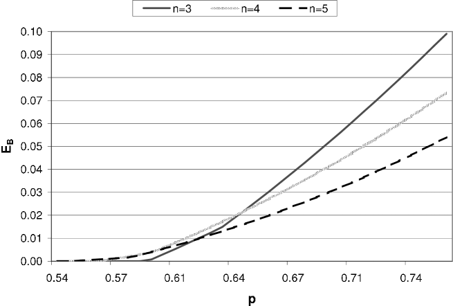
Figure 6: Lower bounds on $E_{B}(\mathcal{E}_{p})$ via n-bit Cat code and modified Cat code. See the text for details.

Note that applying a CNOT gate on the first and the (i-1)th qubits followed by measuring the (i-1)th qubit along the z-axis as shown in figure 5 is the same as measuring $g_{i}$, and we are interested in keeping track of the quantum state of the first qubit that passed through $\mathcal{E}_{p}$ after each measurement $g_{i}$. We are only interested in its quantum state if the measuring result is ‘+1’, since we otherwise discard the states and start all over. Denote this state by $M_{i}$, and we have the following relations 49 :

$$p_{i+1}=(F+G)\bra{\Phi^{+}}M_{i}\ket{\Phi^{+}}+(2G)\bra{\Psi^{+}}M_{i}\ket{\Psi^{+}}+(F+G)\bra{\Phi^{-}}M_{i}\ket{\Phi^{-}}+(2G)\bra{\Psi^{-}}M_{i}\ket{\Psi^{-}}$$

$$\bra{\Phi^{+}}M_{i+1}\ket{\Phi^{+}} = \frac{F\bra{\Phi^{+}}M_{i}\ket{\Phi^{+}}+G\bra{\Phi^{-}}M_{i}\ket{\Phi^{-}}}{p_{i}}$$

$$\bra{\Psi^{+}}M_{i+1}\ket{\Psi^{+}} = \frac{G\bra{\Psi^{+}}M_{i}\ket{\Psi^{+}}+G\bra{\Psi^{-}}M_{i}\ket{\Psi^{-}}}{p_{i}}$$

$$\bra{\Phi^{-}}M_{i+1}\ket{\Phi^{-}} = \frac{G\bra{\Phi^{+}}M_{i}\ket{\Phi^{+}}+F\bra{\Phi^{-}}M_{i}\ket{\Phi^{-}}}{p_{i}}$$

$$\bra{\Psi^{-}}M_{i+1}\ket{\Psi^{-}} = \frac{G\bra{\Psi^{+}}M_{i}\ket{\Psi^{+}}+G\bra{\Psi^{-}}M_{i}\ket{\Psi^{-}}}{p_{i}}$$

where $F=\frac{3p+1}{4}$, $G=\frac{1-F}{3}$ and $M_{n-1}=\omega_{n+1}$. From these equations and (7), we compute the lower bounds on $E_{B}$ with n-bit Cat code and modified Cat code for $n=3,4,5$ in figure 6. Modified Cat code differs from Cat code in the same way that the modified recurrence method differs from the recurrence method. Namely, Bob switches the $\ket{\Phi^{-}}\bra{\Phi^{-}}$ and $\ket{\Psi^{-}}\bra{\Psi^{-}}$ components in the probabilistic mixture of Bell states after each measurement. This can be done by first applying a bilateral $\pi/2$ rotation $B_{x}$ and then a unilateral $\pi$ rotation $\sigma_{x}$ 35 . Modified Cat code outperforms Cat code when the channel is less noisy(large p), but Cat code performs slightly better when the channel is very noisy and hence achieves a lower threshold value. In figure 7, we plot the yield for 4-bit Cat code and modified Cat code separately.

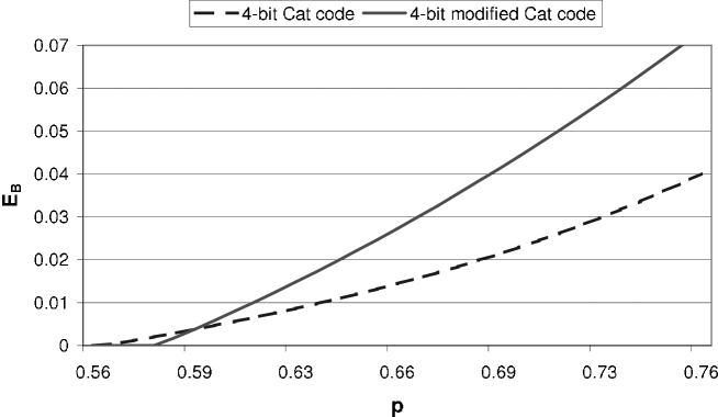
Figure 7: 4-bit Cat code vs. 4-bit modified Cat code.

III.4 Shor code

The generators of Shor code are listed in (6). The logical operators and logical computational basis states are as follows:

$$\bar{X} = Z_{1}Z_{2}Z_{3}Z_{4}Z_{5}Z_{6}Z_{7}Z_{8}Z_{9}$$

$$\bar{Z} = X_{1}X_{2}X_{3}X_{4}X_{5}X_{6}X_{7}X_{8}X_{9}$$

$$\ket{0}_{L} = \frac{(\ket{000}+\ket{111})(\ket{000}+\ket{111})(\ket{000}+\ket{111})}{2\sqrt{2}}$$

$$\ket{1}_{L} = \frac{(\ket{000}-\ket{111})(\ket{000}-\ket{111})(\ket{000}-\ket{111})}{2\sqrt{2}}.$$

As aforementioned, for 9-bit Shor code, the optimal AQECC protocols are slightly different for different levels of noise. We can divide the protocols into 3 regions:

p protocol less than 0.75 start all over if any measurement result is ‘-1’ between 0.75 start all over if any of the first 7 measurement results is ‘-1’; and 0.78 otherwise continue with the regular error-correcting operation great than 0.78 start all over if any of the first 4 measurement results is ‘-1’; otherwise continue with the regular error-correcting operation

In the first region (p less than 0.75), one only has to enumerate all $4^{9}$ error possibilities in the 9 channel uses and adds up all probabilities associated with having an $X$ error, a $Y$ error, a $Z$ error or no error on the encoded qubit. Then the $E_{B}$ rate achieved for $\mathcal{E}_{p}$ is given by:

$$\frac{p_{1}\times p_{2}\times\ldots\times p_{8}\times\big{(}1-H(p{00},p{01},p{10},p{11})\big{)}}{n^{*}}$$

where

$$n^{*} = 2\times(1-p_{1})+3\times p_{1}(1-p_{2})+5\times p_{1}p_{2}(1-p_{3})+6\times p_{1}p_{2}p_{3}(1-p_{4})$$

$$+6\times p_{1}p_{2}p_{3}p_{4}(1-p_{5})+8\times p_{1}p_{2}p_{3}p_{4}p_{5}(1-p_{6})+9\times p_{1}p_{2}p_{3}p_{4}p_{5}p_{6}.$$

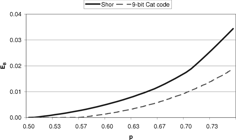
Figure 8: Lower bounds on $E_{B}(\mathcal{E}_{p})$ via 9-bit Shor code and 9-bit Cat code.

In the second and the third region, the computation is slightly different. We will illustrate with the third region, and the computation for the second region is similar. Since Alice and Bob will start all over if any of the first 4 measurement results is ‘-1’, there are only $2^{(8-4)}=16$ possible measurement results given that the whole block of 9 qubits were sent through the channel. Denote the 4-tuple measurement results by $m\in\{0,1,\ldots,15\}$. For each measurement result, Bob will carry out error-correcting operation as in the standard 9-bit Shor code and inform Alice which of the 16 measurement results this block of 9 qubits has. Then after a large number of 9-bit blocks are transmitted successfully, Alice and Bob share a large number of each of the 16 types of Bell-diagonal probabilistic mixtures so that they can perform universal hashing on each of these 16 types of mixtures separately. And the $E_{B}$ rate achieved is given by

$$\sum_{m}\Bigg{(}\frac{1}{n^{**}}\textrm{ prob(measurement result is m) }\bigg{(}1-H(p{00},p{01},p{10},p{11}|m)\bigg{)}\Bigg{)}$$

where $H(p{00},p{01},p{10},p{11}|m)$ is the entropy of the probabilistic mixture given a particular measure result $m\in\{0,1,\ldots,15\}$ has occurred and $n^{**}=2\times(1-p_{1})+3\times p_{1}(1-p_{2})+5\times p_{1}p_{2}(1-p_{3})+6\times p_{1}p_{2}p_{3}(1-p_{4})+9\times p_{1}p_{2}p_{3}p_{4}$. In figure 8, we plot the $E_{B}$ rate achieved; for comparison $E_{B}$ rate achieved for 9-bit Cat code is also shown.

III.5 Modified recurrence method

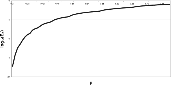
Figure 9: Lower bounds on $E_{B}(\mathcal{E}_{p})$ via the modified recurrence method.

Modified recurrence method as described in 35 is a 2-EPP which requires two-way classical communication. Although Alice can perform the measurement before she sends halves of the EPR pairs $\ket{\Phi^{+}}$ through $\mathcal{E}_{p}$ so that Bob need not know her measurement results in the first round, as we discussed in section III.3 and III.4, an iterative process is not possible. In particular, one round of recurrence plus universal hashing via the classical feedback channel achieve positive $E_{B}$ rate only for $p>0.638$. If Alice and Bob want to carry out another round of the modified recurrence method, she needs a forward channel to communicate her measurement results to Bob. Since the only forward channel for Alice is $\mathcal{E}_{p}$, a straightforward extension, therefore, is to use the channel $\mathcal{E}_{p}$ to send her measurement results to Bob. As a result, from the second round onwards, one classical bit per pair is required for each round of recurrence.

By proving the additivity conjecture for the quantum depolarizing channel $\mathcal{E}_{p}$, the formula for the classical capacity of $\mathcal{E}_{p}$ is known13 :

$$C(\mathcal{E}_{p})=1+\Big{(}\frac{1+p}{2}\Big{)}\log_{2}\Big{(}\frac{1+p}{2}\Big{)}+\Big{(}\frac{1-p}{2}\Big{)}\log_{2}\Big{(}\frac{1-p}{2}\Big{)}=1-H\Big{(}\frac{1+p}{2},\frac{1-p}{2}\Big{)}.$$

Then the $E_{B}$ yield implied by this method for $k$ rounds of recurrence before switching to universal hashing is given by:

$$\Bigg{(}\frac{p_{pass}^{(1)}}{2}\Bigg{)}\times\Bigg{(}\frac{p_{pass}^{(2)}}{2+1/C(\mathcal{E}_{p})}\Bigg{)}\times\ldots\Bigg{(}\frac{p_{pass}^{(k)}}{2+1/C(\mathcal{E}_{p})}\Bigg{)}\times\Bigg{(}1-H\Big{(}p_{00}^{(k)},p_{01}^{(k)},p_{10}^{(k)},p_{11}^{(k)}\Big{)}\Bigg{)}$$

where $p_{00}^{(k)}$, $p_{01}^{(k)}$, $p_{10}^{(k)}$, $p_{11}^{(k)}$ and $p_{pass}^{(i)}$ for $i=1,2,\ldots,k$ are given by the recurrence relations (3) and (4) in section I.2.2. In figure 9, we plot the $E_{B}$ rate achieved by this method.

III.6 Leung-Shor method

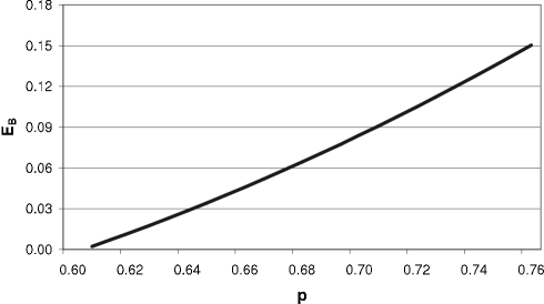
Figure 10: Lower bounds on $E_{B}(\mathcal{E}_{p})$ via the Leung-Shor method.

The Leung-Shor methodLS1 introduced in section I.2.3 is in fact an $E_{B}$ protocol. Alice only needs to encode the qubits into what they would have been if the measurement results in figure 2 were both ‘+1’. In figure 10, we plot the $E_{B}$ rate achieved. In figure 11, we compare the yield of the four methods in this section.

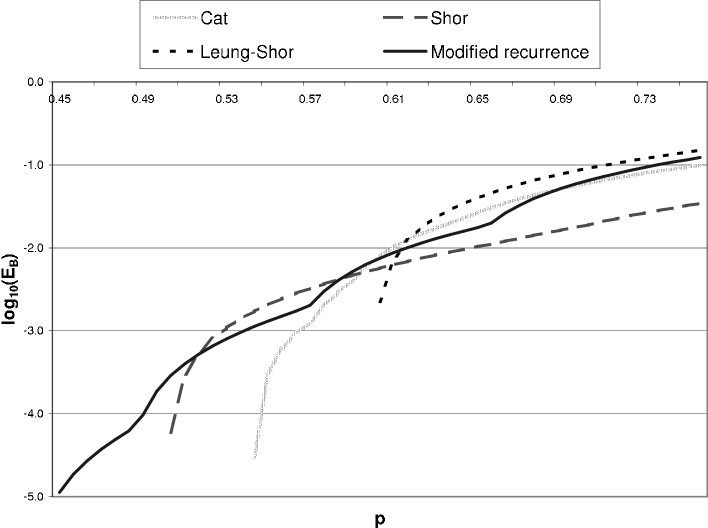
Figure 11: Lower bounds on $E_{B}(\mathcal{E}_{p})$.

IV New lower bounds on $Q_{B}$

We will establish the following lemma which gives lower bounds on $Q_{B}$ based on $E_{B}$ protocols:

Lemma 2

$$Q_{B}(\mathcal{E}_{p}) \geq \frac{C(\mathcal{E}_{p})}{1+\frac{C(\mathcal{E}_{p})}{E_{B}(\mathcal{E}_{p})}}$$

where $C(\mathcal{E}_{p})=1-H\big{(}\frac{1+p}{2},\frac{1-p}{2}\big{)}.$

Proof In an $E_{B}$ protocol, Alice and Bob share M EPR pairs $\ket{\Phi^{+}}$ in N channel uses. Therefore, $E_{B}(\mathcal{E}_{B})=M/N$. To teleport a quantum state $\rho\in\mathcal{H}_{2}^{\otimes M}$, Alice can use the channel $\mathcal{E}_{p}$ for $\frac{M}{C(\mathcal{E}_{p})}$ many times to send M bits of classical information to Bob. Thus,

$$Q_{B}(\mathcal{E}_{p}) \geq \frac{M}{N+\frac{M}{C(\mathcal{E}_{p})}}=\frac{M/N}{1+\frac{M/N}{C(\mathcal{E}_{p})}}$$

$$= \frac{E_{B}(\mathcal{E}_{p})}{1+\frac{E_{B}(\mathcal{E}_{p})}{C(\mathcal{E}_{p})}}=\frac{C(\mathcal{E}_{p})}{1+\frac{C(\mathcal{E}_{p})}{E_{B}(\mathcal{E}_{p})}}.$$

$\square$

From the lemma, any lower bounds on $E_{B}$ will imply lower bounds on $Q_{B}$. The lower bounds are presented in figure 12.

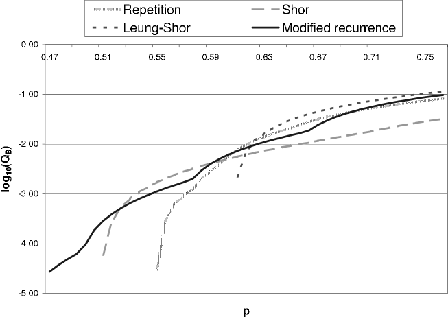
Figure 12: Lower bounds on $Q_{B}(\mathcal{E}_{p})$.

V Threshold of Cat code

It has been shown that in the absence of side classical communication one can achieve non-zero capacity for lower threshold fidelity $F=\frac{3p+1}{4}$ by concatenating 5-bit Cat code inside a random code (hashing)50 . Threshold fidelity for concatenating n-bit Cat code into random code was also studied. It was found that threshold fidelities fall into two smooth curves, one for even n and one for odd n, but both curves increase with n, i.e. one does not attain lower threshold by using a longer Cat code. We therefore compute the threshold fidelity for n-bit Cat code in figure 13 and we found that these phenomena do not occur in AQECC.

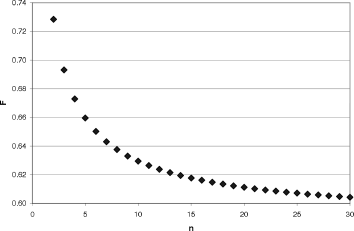
Figure 13: Threshold fidelity $F=\frac{3p+1}{4}$ for n-bit Cat code.

VI Discussion on $Q_{B}$, $E_{B}$ and $Q_{2}$

In this work, we defined the quantum entanglement capacity with classical feedback $E_{B}$ for any quantum discrete memoryless channel. For any channel, this quantity was shown to lie between two other capacities, namely the quantum capacity with classical feedback $Q_{B}$ and the quantum capacity with two-way classical communication $Q_{2}$. It is an open question whether there exists quantum channel for which $Q_{2}>Q_{B}$. While the introduction of this new, intermediate quantity $E_{B}$ does not simplify the question, it is our hope to shed some light on and provide other means to tackle this open problem. In section II, we provided an alternate operational interpretation of this quantity: it represents the amount of quantum information Bob can send to Alice. It is our hope that, by working with this interpretation, one might be able to prove a non-trivial upper bound on $E_{B}$ and hence lead to a separation between $Q_{B}$ and $Q_{2}$.

We converted many of the well-known QECC into $E_{B}$ protocols and computed their yields. These in turn led to new lower bounds on $Q_{B}$. The QECC that we studied, namely Cat code and Shor code, exhibit different behaviors under this AQECC framework. For example, for Shor code, it is beneficial to not insist on getting no error in all measurements but instead carry out error-correcting procedures after getting no error in the first few measurements. Whereas for Cat code, one has to insist on getting no error in all measurements. It is interesting to study which of these two features is exhibited by other codes.

We also saw some connections with 2-EPP. Firstly, even though the Leung-Shor method was introduced in LS1 as a 2-EPP, it is in fact an $E_{B}$ protocol. Secondly, when the idea of modified recurrence method is applied to Cat code, higher $E_{B}$ yields are achieved.

Finally, one may want to ask whether the threshold fidelity in section V goes down monotonically and if it does, to what value it converges as n goes to infinity.

After the completion of this work, the conjectural relation $Q_{2}>Q_{B}$ was proved N24 , and an emerging question is whether the relation $Q_{2}>Q_{B}$ holds for all quantum channels except when both capacities vanish. Also, can one show a separation between $E_{B}$ and $Q_{2}$?

Acknowledgements: the author is grateful to Peter Shor for his important insights during the course of this work, and would like to thank Charles Bennett for his advice on the recent developments.

References

- (1) C.H. Bennett and P.W. Shor, Quantum Information Theory, IEEE Trans. Inform. Theory, vol. 44, p.2724 to 2742, 1998
- (2) M.A. Nielsen and I.L. Chuang, Quantum Computation and Quantum Information (Cambridge University Press, 2000)
- (3) T.M. Cover and J.A. Thomas, Elements of Information Theory (John Wiley and Sons, New York, 1991)
- (4) C.E. Shannon, A mathematical theory of communication, The Bell System Tech. J., vol. 27, p. 379 to 423, 623 to 656, 1948
- (5) C.H. Bennett, I. Devetak, P.W. Shor and J.A. Smolin, Inequalities and Separations among Assisted Capacities of Quantum Channels, quant-ph/04-06-086
- (6) C.H. Bennett, P.W. Shor, J.A. Smolin and A.V. Thapliyal, Entanglement-Assisted Classical Capacity of Noisy Quantum Channels, Phys. Rev. Lett., vol. 83, p.3081 to 3084, 1999, quant-ph/99-04-023
- (7) C.H. Bennett, P.W. Shor, J.A. Smolin and A.V. Thapliyal, Entanglement-Assisted Capacity of a Quantum Channel and the Reverse Shanno Theorem, quant-ph/01-06-052
- (8) C.H. Bennett, D.P. DiVincenzo and J.A. Smolin, Capacities of Quantum Erasure Channels, quant-ph/97-01-015
- (9) C. King, The capacity of the quantum depolarizing channel, quant-ph/02-04-172
- (10) I. Devetak, The private classical capacity and quantum capacity of a quantum channel, to appear in IEEE Trans. Inform. Theory, quant-ph/03-04-127
- (11) P. Hausladen, R. Jozsa, B. Schumacher, M. Westmoreland and W.K. Wootters, Classical information capacity of a quantum channel, Phys. Rev. A, vol. 54, p.1869 to 1876, 1996
- (12) B. Schumacher and M.D. Westmoreland, Sending classical information via noisy quantum channels, Phys. Rev. A, vol. 54, p.2629 to 2635, 1996
- (13) P.W. Shor, The Classical Capacity Achievable by a Quantum Channel Assisted by Limited Entanglement, quant-ph/04-02-129
- (14) C. King, Additivity for unital qubit channels, quant-ph/01-03-156
- (15) C. King, An application of a matrix inequality in quantum information theory, quant-ph/04-12-046
- (16) P.W. Shor, Equivalence of Additivity Questions in Quantum Information Theory, quant-ph/03-05-035
- (17) P.W. Shor, Additivity of the classical capacity of entanglement breaking quantum channels, quant-ph/02-01-149
- (18) G. Bowen and R. Nagarajan, On Feedback and the Classical Capacity of a Noisy Quantum Channel, IEEE Trans. Inform. Theory, vol.51, p.320 to 324, 2005, quant-ph/03-05-176
- (19) C.H. Bennett, D.P. DiVincenzo, J.A. Smolin and W.K. Wootters, Mixed State Entanglement and Quantum Error Correction, Phys. Rev. A, 54, pp. 3824-3851 (1996), quant-ph/96-04-024
- (20) E. Hostens, J. Dehaene and B.D. Moor, Asymptotic adaptive bipartite entanglement distillation protocol, quant-ph/0602205
- (21) A.W. Leung and P.W. Shor, Entanglement Purification with Two-way Classical Communication, to appear in Quantum Information and Computation
- (22) E.N. Maneva and J.A. Smolin, Improved two-party and multi-party purification protocols, quant-ph/00-03-099
- (23) K.G.H. Volbrecht and Frank Verstraete, Interpolation of recurrence and hashing entanglement distillation protocols, quant-ph/0404111
- (24) R.F. Werner, Quantum states with Einstein-Podolsky-Rosen correlations admitting a hidden-variable model, Phys. Rev. A, 40, pp. 4277-4281 (1989)
- (25) C.H. Bennett, G. Brassard, S. Popescu, B. Schumacher, J.A. Smolin and W.K. Wooters, Purification of Noisy Entanglement and Faithful Teleportation via Noisy Channels, Phys. Rev. Lett., 76, pp. 722-725 (1996)
- (26) H. Barnum, E. Knill and M.A. Nielsen, On Quantum Fidelities and Channel Capacities, IEEE Trans. Inform. Theory, vol. 46, p.1317 to 1329, 2000, quant-ph/98-09-010
- (27) E. Knill and R. Laflamme, Theory of quantum error-correcting codes, Phys. Rev. A, vol. 55, pp. 900 to 911, 1997
- (28) P.W. Shor, Scheme for reducing decoherence in quantum computer memory, Phys. Rev. A, vol. 52, pp.2493, 1995
- (29) A.M. Steane, Error correcting codes in quantum theory, Phys. Rev. Lett., vol. 77, pp.793, 1996
- (30) D. Bacon, Operator quantum error-correcting subsystems for self-correcting quantum memories, quant-ph/05-060-23
- (31) D.W. Kribs, R. Laflamme, D. Poulin and M. Leosky, Operator quantum error correction, quant-ph/05-04-189
- (32) D.P. DiVincenzo, P.W. Shor and J.A. Smolin, Quantum channel capapcity of very noisy channels, quant-ph/97-06-061
- (33) P.W. Shor and J.A. Smolin, Quantum error-correcting codes need not completely reveal the error syndrome, quant-ph/96-04-006
- (34) D.W. Leung, J. Lim and P.W. Shor, On quantum capacity of erasure channel assisted by back classical communication, quant-ph/07-10-5943