Propagation of a quantum particle through two dimensional percolating systems

Abstract

We study quantum percolation which is described by a tight-binding Hamiltonian containing only off-diagonal hopping terms that are generally in quenched binary disorder (zero or one). In such a system, transmission of a quantum particle is determined by the disorder and interference effects, leading to interesting sharp features in conductance as the energy, disorder, and boundary conditions are varied. To aid understanding of this phenomenon, we develop a visualization method whereby the progression of a wave packet entering the cluster through a lead on one side and exiting from another lead on the other side can be tracked dynamically. Using this method, we investigate the evolution of the wave packet through transmission and reflection under clusters of various disorder, sizes, boundary conditions, and energies. Our results indicate the existence of two different kinds of localized regimes, namely exponential and power law localization, depending on the amount of disorder. Our study further suggests that there may be a delocalized state in the 2D quantum percolation system at very low disorder. These results are based on a finite size scaling analysis of the systems of size up to $70\times 70$ (containing 4900 sites) on the square lattice.

I Introduction

The transmittance of a classical particle through a disordered system depends solely on the availability of a spanning path through the system. This criterion, however, must be modified generally for a quantum particle since interference and tunneling effects must be included for a quantum system. In particular, the presence of a spanning path does not by itself ensure the transmittance of a quantum particle because of the interference effect. Even for a completely ordered system, a quantum particle may exhibit zero transmission depending on the details such as the energy of the particle cuansing:04 . Our quantum percolation system includes the interference effect fully but does not include any of the tunneling effect; thus we expect a higher connectivity in underlying geometry to be required for non-zero transmission compared to its classical counterpart.

A major motivation for studying such a system is the question of whether a localized- to-delocalized (or perhaps, metal-to-insulator) transition exists in a two-dimensional (2D) system. The Anderson model and the quantum percolation model are two of the more common theoretical models that are used to study the transport properties of disordered systems. While the literature on both models agree on the existence of such a transition in three dimensions,souk:87 ; kosl:91 ; berk:96 , the same question for quantum percolation in two dimensions appears to have remained a subject of controversy for over two decades. Based on the scaling theory of Abrahams et al abrahams:79 , it was widely believed that there can be no metal-to-insulator transition in 2D universally in the absence of a magnetic field or interactions for any amount of disorder.goldenfeld However, whether this theory also applies to quantum percolation has been debated in recent years.

In the mean time, experiments performed in early 1980’s on different 2D systems exp:1 ; exp:2 ; exp:3 confirmed the scaling theory predictions. However, a number of experiments that appeared more recently seem to suggest that a metallic state may be possible in two dimensions. For reviews of these experiments, see Abrahams et al. abrahams:01 and references therein. In this work, we do not address the issues of these experiments, but rather concentrate on the formally much simpler quantum percolation model which has neither magnetic field nor interactions but contains binary disorder with infinite barriers at randomly diluted sites.

We study the behavior of 2D quantum percolation systems by tracking how a wave packet, representing a quantum particle, evolves with time as it enters a diluted 2D system through a 1D lead. Even restricting attention to quantum percolation which lacks many effects that are expected to play important roles in metal-insulator transitions, there is a long-standing controversy as to the presence or absence of an extended state and of a phase transition between the prevalent localized state and a more elusive extended state in two-dimensions. On one hand, some studies such as those made using the dlog Padé approximation method daboul:00 , real space renormalization method odagaki84 , and the inverse participation ratio srivastava84 found a transition from exponentially localized states to non-exponentially localized states for a range of site concentrations between $0.73\leq p_{q}\leq 0.87$ on the square lattice. So did a study of energy level statistics letz:99 , one of the spread of a wave packet initially localized at a site nazareno:02 , and one of a transfer matrix eilmes:01 , where the nature of the delocalized state remained not fully understood. On the other hand, studies such as the scaling work based on numerical calculation of the conductance haldas02 , the investigation of vibration-diffusion analogy bunde98 , finite-size scaling analysis and transfer matrix methods soukoulis91 , and vector recursion technique mookerjee95 found no evidence of a transition. A study by Inui et al. inui94 found all states to be localized except for those with particle energies at the middle of the band and when the underlying lattice is bipartite, such as a square lattice. More recently, Cuansing and Nakanishi (private communication) used an approach first suggested by Daboul at al. daboul:00 to calculate conductance directly for clusters of several hundred sites and, extrapolating those results by finite- size scaling, suggested that delocalized states exist and thus a transition would have to exist as well.

To aid understanding of transport of a quantum particle in 2D systems, we have developed a new dynamical visualization method. It is based on usual scattering process where we let a particle, described by a Gaussian wave packet, enter into the system (sometimes called a cluster) through an input lead and track how it propagates through the system and exits from the other side of the cluster through the output lead. Thus by determining the transmission probability we can acquire valuable information about the cluster. The method is very useful to study the characteristics of ordered as well as disordered clusters. It clearly demonstrates the effect of interference on propagation which is a unique feature of a quantum system. A great utility of this method is that we can visualize the progression of the wave packet in real time and investigate the nature of localization of a particle in 2D quantum percolation system.

We have used the tool we have developed to study behavior of a particle both in square and triangular lattices. However, most of the work presented in this paper is for a 2D system realized on the square lattice. In Section II, we discuss the method we have developed to study 2D systems. In Sections III and IV we present the application of this method to ordered and disordered quantum percolation systems respectively. And finally we present our conclusion in Section V.

II The Model and Numerical approach

We study quantum percolation that is described by

$$H=\sum_{<ij>}V_{ij}|i\rangle{\langle}j|+h.c$$ (1)

where $|i>$ and $|j>$ are tight binding basis functions at sites $i$ and $j$, respectively and $V_{ij}$ is the hopping matrix element which is 1 if $i$ and $j$ are nearest neighbors, otherwise zero. We realized this model on both square and triangular lattices that can have at most 4 and 6 nearest neighbors respectively. In ordered cases, all lattice sites are available and included in the sum, while in disordered cases, we randomly dilute (or remove) a certain fraction of the lattice sites and consider them not available (and excluded from the sum).

To study the propagation of a quantum particle we connect two 1D leads, one as input and the other one as output lead, to the 2D cluster, and construct a Gaussian wave packet in the input chain that represents the incident particle. The usual time dependent Schrödinger equation is then solved for this system.

$$i\frac{\partial\psi(r,t)}{\partial t}=H\psi$$ (2)

Here,

$$\psi(r,t=0)=(const.)\cdot\mbox{e}^{(r-r_{0})^{2}/(4s^{2})}\cdot\mbox{e}^{-ik_{0}r}$$ (3)

(on input chain only) and $s$ is the width of the wave packet, $k_{0}$ is the central wave vector of the wave packet and $r_{0}$ is the location of the center of the wave packet in the input chain. For all simulations in this work we construct the wave packets with $s$ which corresponds to 4 lattice spacings and $r_{0}$ at the middle of the input chain. These choices assure that $k_{0}$ is a well-defined mean wave vector of the incoming wave packet.

Allowing this wave packet to evolve with time under this Hamiltonian we can study its transmission characteristics. For simulation purposes, Eq. 2 is converted to a discrete form as follows nakanishi:05 . We write the wave function in terms of its real and imaginary parts and upon substitution back into Eq. 2 this gives two coupled equations:

$$\psi(r,t)=R(r,t)+iI(r,t)$$ (4)

$$\frac{\partial R(r,t)}{\partial t}=H\cdot I(r,t)$$ (5)

$$\frac{\partial I(r,t)}{\partial t}=-H\cdot R(r,t)$$ (6)

We then apply a leap-frog method to arrive at the discrete forms of these two equations,

$$I(r,t+\frac{1}{2})\approx I(r,t-\frac{1}{2})-\triangle t\cdot H\cdot R(r,t)$$ (7)

$$R(r,t+1)\approx R(r,t)+\triangle t\cdot H\cdot I(r,t+\frac{1}{2})$$ (8)

We have used MATLAB graphics tools to visualize this dynamical process.

III Propagation through a completely ordered system

III.1 Square Lattice

We have applied the method described in the previous section to investigate first the behavior of a quantum particle in an ordered 2D system. In this context, ordered means that all lattice sites of the system are available to the particle. The cluster has been studied using two different types of the connection of the leads. In the point-to-point contact, the input lead is connected to only one site on the input side of the cluster and the output lead is connected to only one lattice site on the opposite side of the cluster. In the busbar type contact, all the lattice points on the input side of the cluster are connected to the input lead, while all the lattice points on the output side of the cluster are connected to the output lead (Fig. 1).

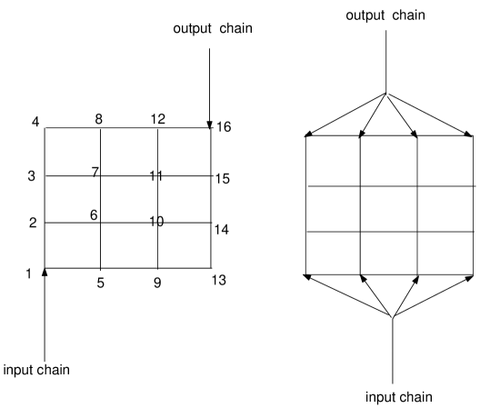
(a)                                   (b)

Figure 1: $4\times 4$ Square Lattice: (a) point to point connection and (b) busbar type connection. The numbers are the labels of the lattice points of the cluster used to construct the Hamiltonian (Eq. 1). The same sequence of labeling is used for all sizes of the clusters used in this work.

There are many possible ways one can arrange a point-to-point connection and transmission is affected by the details of the leads’ connection to the cluster. One such arrangement is shown in Fig. 2, where a packet propagates through diagonally connected leads. We generate a wave packet centered in the middle of the input lead with a central wave vector $k_{0}$ = 4.3 (in units of inverse lattice constant). As the wave packet spreads and propagates through the cluster, it interferes with itself in many ways. This interference effect is particularly large when the wave packet reaches the contact point with the output lead (Fig. 2c). A part of the wave packet is reflected back to the cluster from the contact and surrounding edges of the cluster, thereby reducing transmission. The calculation of the transmission coefficient $T$ requires some approximation in this approach. In most of what follows, we estimate $T$ by summing the portion of the normalized wave packet that is on the output lead when the leading edge of the wave packet has first reached the end of the output lead. Often we can visually confirm the validity of this method by looking at the evolution of the wave packet shape explicitly, but in addition, we have also first employed increasing lead lengths to locate an optimal length where this approximation yields stable values of $T$ and then used this optimal length in our later work.

$\begin{array}[]{cc}{\leavevmode\resizebox{231.26378pt}{144.54pt}{\includegraphics{p2f2a.eps}}}&{\leavevmode\resizebox{231.26378pt}{144.54pt}{\includegraphics{p2f2b.eps}}}\\ (a)&(b)\\ {\leavevmode\resizebox{231.26378pt}{144.54pt}{\includegraphics{p2f2c.eps}}}&{\leavevmode\resizebox{231.26378pt}{144.54pt}{\includegraphics{p2f2d.eps}}}\\ (c)&(d)\end{array}$

Figure 2: A typical time evolution of a wave packet through a cluster of size $20\times 20$ with leads connected diagonally at the lower left and upper right corners of the cluster. The time step for each snapshot and corresponding reflection and transmission coefficients $R$ and $T$ are shown at the top of each snapshot.

Another important feature that is evident from Fig. 2 is that, unlike a classical particle, a quantum particle has a non-zero probability to be observed at any part of the system at any instant of time. However, since we are most interested in the behavior of the particle inside the cluster, from now on we shall visualize only the cluster part of the wave packet.

To study the effect of energy of the incident particle on transmission, we have calculated the transmission coefficient for a range of central wave vectors of the particle. Since we are interested in the behavior of the cluster in thermodynamic limit, we also have investigated how the size of the cluster as well as the leads affect transmission. We have studied three different sizes of clusters, namely $20\times 20$, $30\times 30$ and $70\times 70$ with four different sizes of the leads, 50, 100, 150 and 200 connected diagonally with the clusters. For each cluster-lead combination we have calculated transmission, T, by varying the central wave vector from 0.5 to 10 (in units of inverse lattice constant) in increments of 0.05. The width, $s$, of the incident packet in all these cases is taken to be equal to 4 lattice constants. Since the largest size of the clusters considered in this work is $70\times 70$, we present in Fig. 3 the results only for $70\times 70$ cluster.

$\begin{array}[]{cc}{\leavevmode\resizebox{231.26378pt}{180.67499pt}{\includegraphics{p2f3a.eps}}}&{\leavevmode\resizebox{231.26378pt}{180.67499pt}{\includegraphics{p2f3b.eps}}}\\ (a)&(b)\end{array}$

Figure 3: The effect of the central wave vector of the wave packet on transmission through cluster of size $70\times 70$ connected to leads of length (a) 80 and (b) 150.

The above study suggests that the length of the leads does not have a major effect on propagation beyond some finite length. For certain values of the central wave vector, $k_{0}$, particle shows resonance transmission and $T$ reaches its maximum value. It is also evident that a quantum particle may show zero transmittance even when the cluster is completely ordered, a characteristic commonly known as resonance reflection. These resonances are similar to the ones found by Cuansing and Nakanishi. cuansing:04

When the leads are connected to edge sites other than the diagonal corners, transmission is generally reduced significantly. Fig. 4 shows the time evolution of the same wave packet as in Fig. 2 when the input lead is connected to the $5^{th}$ lattice point (input side) and the output lead is at $15^{th}$ lattice point (output side) of the cluster. The reason for this decrease in transmission is obvious from Fig. 4. As the wave packet enters the cluster, it now spreads broadly throughout the whole cluster and consequently only a small part of it reaches the output lead.

$\begin{array}[]{ccc}{\leavevmode\resizebox{231.26378pt}{180.67499pt}{\includegraphics{p2f4a.eps}}}&{\leavevmode\resizebox{231.26378pt}{180.67499pt}{\includegraphics{p2f4b.eps}}}\end{array}$

Figure 4: The time evolution of a wave packet through square cluster of size $20\times 20$ with off diagonally connected leads.

The wave vector dependence of transmission for off-diagonally connected leads is shown in Fig. 5. The dependence is quite different from what we have observed in the case of the diagonal connection. The peak values of $T$ are significantly reduced and the locations of the peaks are shifted as well, though the same periodicity still exists as it must.

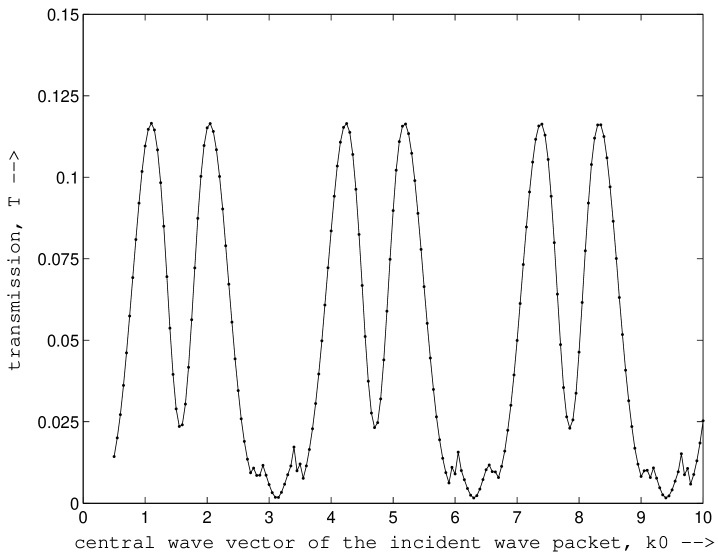
Figure 5: The effect of the central wave vector of the wave packet on transmission through cluster of size $70\times 70$ with input lead at $5^{th}$ lattice point on the input side and output lead at $65^{th}$ lattice point on the output side of the cluster.

The propagation of the wave packet under busbar type connection, on the other hand, is dominated by the destructive interference of the packet on the edge of the cluster at the input contact and very little transmission is observed (Fig. 6). As before we display a packet centered about $k_{0}$ = 4.3 (in units of inverse lattice constant) with cluster size $20\times 20$. For certain energies, however, transmission is significantly large (resonance transmission).

$\begin{array}[]{cc}{\leavevmode\resizebox{231.26378pt}{144.54pt}{\includegraphics{p2f6a.eps}}}&{\leavevmode\resizebox{231.26378pt}{144.54pt}{\includegraphics{p2f6b.eps}}}\\ \end{array}$

Figure 6: Transmission under busbar connection through a $20\times 20$ square cluster.

III.2 Triangular Lattice

Though most of the results obtained in this work is based on square lattice, we have also investigated the propagation of the particle on triangular lattice. The triangular lattice (Fig. 7) differs from the square lattice in that it has 6 nearest neighbors for each lattice point and thus much higher local connectivity. It is also not bipartite and thus may avoid features that are only present on bipartite structures.inui94

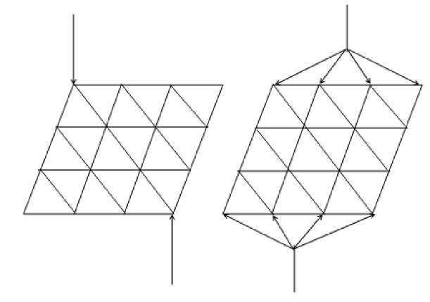
(a)                                  (b)

Figure 7: $4\times 4$ Triangular Lattice: (a) point to point connection and (b) busbar type connection.

While there are many more paths available for a particle on triangular lattice than on square lattice, this may not necessarily lead to higher transmission unlike in classical transport since the interference effect may is also expected to be larger. We repeated our simulation shown in Fig. 2 for the triangular lattice. As is evident from the sample time evolution shown in Fig. 8 with diagonally connected leads, the spread of the wave packet throughout the cluster is aided by the availability of additional paths. We found that these effects generally result in lower transmission for the diagonal connection. However, transmission increases with the busbar-type connection, which makes the difference in transmission between these two connection types to be much smaller than for the square lattice.

$\begin{array}[]{cc}{\leavevmode\resizebox{231.26378pt}{180.67499pt}{\includegraphics{p2f8a.eps}}}&{\leavevmode\resizebox{231.26378pt}{180.67499pt}{\includegraphics{p2f8b.eps}}}\\ \end{array}$

Figure 8: The time evolution of the wave packet through $20\times 20$ triangular lattice with diagonally connected leads.

IV The effect of disorder on transmission

Everything we have described so far was for completely ordered system. The main reason why we have started this work is to visualize the effect of disorder on transmission. As a first step towards understanding that, we investigate how propagation is affected by prefixed dilution. A site is diluted by removing it from the cluster, thus making it unavailable for hopping to. The diluted sites act as infinite potential barriers for the particle. We start with a single diluted site in a $20\times 20$ cluster and observe how the wave packet with central wave vector $k_{0}$ = 4.3 (in units of inverse lattice constant) evolves with time. The Fig. 9 shows some snapshots of the wave packet with a diluted site located at $86^{th}$ lattice site which is close to the body diagonal of the cluster.

$\begin{array}[]{ccc}{\leavevmode\resizebox{216.81pt}{180.67499pt}{\includegraphics{p2f9a.eps}}}&{\leavevmode\resizebox{216.81pt}{180.67499pt}{\includegraphics{p2f9b.eps}}}\\ \end{array}$

Figure 9: Time evolution of a wave packet propagation is shown in the presence of a single diluted site at the 86th lattice site near the body diagonal. The input and output leads are connected diagonally and this figure should be compared with Fig. 2 for the corresponding time evolution without any dilution.

As the wave packet encounters the diluted site, it gets scattered by the infinite barrier and consequently transmission is reduced. We investigated the effect for other diluted sites and our study suggests that transmission is most strongly affected if the diluted sites are close to the body diagonal of the cluster if the leads are connected diagonally with the cluster. Such effects are illustrated in Fig. 9 which should be compared with Fig. 2 for the corresponding time evolution without dilution. The much broader spreading of the wave packet is clearly observed in Fig. 9 as well as in the corresponding values of $T$.

While the effect of dilution is generally to reduce transmission through the cluster for diagonally connected leads, it may enhance transmission at least for some off-diagonally connected leads. If we repeat the simulation shown in Fig. 4 with 3 diluted sites at $27^{th}$, $376^{th}$ and $396^{th}$ lattice points, the propagation appears as shown in Fig. 10 (Since sites are labeled with numbers as illustrated in Fig. 1, these sites are off-diagonal and near either point of contact with the input and output chains). Though the qualitative pictures of the extent of the wave packet spreading appear similar in Fig. 4 (without dilution) and Fig. 10 (with 3 sites diluted), the corresponding values of $T$ at the 100th time step show that transmission is actually enhanced in the presence of these diluted sites.

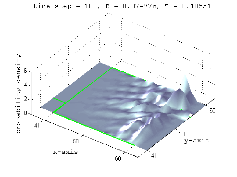
Figure 10: Propagation in the presence of 3 diluted sites for an off-diagonal connection of the leads, where the input lead is connected to the $5^{th}$ lattice point on the input side of the cluster and the output lead is connected to $15^{th}$ lattice point on the output side of the cluster.

The study of propagation under the dilution of specific sites gives us some clue on how disorder may affect propagation through the cluster. We introduce disorder in our system by removing sites from the cluster randomly with a given probability. For instance, a $10\%$ disorder means a site is removed if a random number, uniformly generated between 0 and 1, associated with that site is less than 0.1. The Fig. 11 shows two independent realizations of propagation through a cluster of size $30\times 30$ with $10\%$ disorder with diagonally connected leads. As noted in the figure, the values of transmission $T$ varies widely from realization to realization. If the concentration of diluted sites near the input lead is large then the reflection coefficient is observed to be large. Another important observation is that a large part of the wave packet is trapped inside the disordered cluster.

$\begin{array}[]{cc}{\leavevmode\resizebox{231.26378pt}{158.99377pt}{\includegraphics{p2f11a.eps}}}&{\leavevmode\resizebox{231.26378pt}{158.99377pt}{\includegraphics{p2f11b.eps}}}\\ \hskip 216.81pt(a)\\ {\leavevmode\resizebox{231.26378pt}{158.99377pt}{\includegraphics{p2f11c.eps}}}&{\leavevmode\resizebox{231.26378pt}{158.99377pt}{\includegraphics{p2f11d.eps}}}\\ \hskip 216.81pt(b)\\ \end{array}$

Figure 11: Propagation of a wave packet through a $30\times 30$ cluster with $10\%$ disorder with diagonally connected input and output leads. (a) and (b) are two independent realizations. Note that the values of $T$ vary a great deal in the two realizations although there are similarities in the qualitative features of the wave packet spreading.

This method can be used to study the presence or absence of a localized-delocalized transition in 2D disordered quantum percolation system. As a first step we have applied this method to study the behavior of a particle under different amount of disorder for a given cluster. For most of the work that follows we have used diagonally connected leads of length 80 and a wave packet of central wave vector $k_{0}$ = 4.7 (in units of inverse lattice constant) with width $s$ = 4 lattice constants. To minimize the effect of the boundary on the interior property of the disordered clusters, we made good contacts by keeping the nine sites nearest to both the input and the output contact points always occupied (and available). We considered two different sizes of clusters, $30\times 30$ and $50\times 50$ and for each size and each dilution, 100 independent realizations are used to obtain average values of $T$. The results are plotted in Fig. 12.

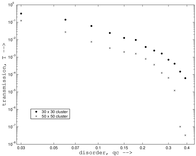
Figure 12: Dependence of transmission $T$ on disorder is illustrated for clusters of size $30\times 30$ and $50\times 50$. Every data point is the average over 100 independent realizations. The apparent onset of a sharp fall in $T$ as disorder increases motivates our closer look as given in the remainder of this work.

We observe from Fig. 12 that the rate of decrease in transmission as disorder is increased is small if disorder is below about $20\%$ but, as the disorder increases beyond $20\%$, transmission begins to fall sharply. This suggests that even if there is no localized-delocalized transition in 2D, the nature of localization of the particle in the disordered cluster may not be the same at all strengths of disorder.

To study the presence or absence of a delocalization transition, one needs to investigate the behavior of the 2D system in thermodynamic limit. This, however, is not possible in numerical methods, and therefore, we resort to a finite size scaling approach in which we calculate the transmission while gradually increasing the size of the system for a given amount of disorder. The result is then extrapolated to study the bulk behavior in the thermodynamic limit. We first obtain the transmission curves for many levels of disorder with the leads connected diagonally with the cluster. The scaling results for this simulation are plotted in Fig. 13 where each data point is the average of 100 disorder realizations. The errors associated with most points are smaller than the symbols used except for those few cases where they are explicitly shown in the plot. In this work, the maximum size of the cluster that could be reached was $70\times 70$.

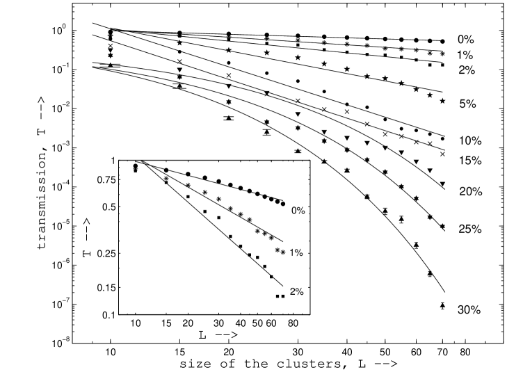
Figure 13: The finite-size scaling of transmission through disordered clusters with diagonally connected leads. In the main panel a log-log plot of $T$ vs $L$ is shown for various amounts of disorder. The solid lines are from the fits made on the log-log scale resulting in the parameters summarized in Table 1, and the standard errors of the mean are smaller than the size of the symbols except where explicitly plotted. The inset shows the the transmission curves only for low disorders (up to 2%) with an expanded scale in the vertical direction. Every data point is the average over 100 realizations.

We have attempted to fit the results to power laws and exponentials in all cases and found that either one of these functions fits clearly better than the other in different regions of the disorder. The resulting best fits are plotted in Fig. 13, and the best fitting parameters are summarized in Table 1 together with the fitting ranges for the $95\%$ confidence bounds in parentheses.

Table 1: Table for fitting parameters performed on the log-log scale for diagonally connected leads without allowing for a possibility of a non-zero offset. Shown in the parentheses are the lower and upper bounds for 95% confidence level.

Disorder	Fit	Parameters		$|R|^{2}$
	equation	a	b
$0\%$		1.96 (1.72, 2.23)	0.30 (0.27, 0.34)	0.97
$1\%$		4.71 (3.26, 6.79)	0.66 (0.56, 0.76)	0.95
$2\%$	$T=a\cdot L^{-b}$	10.7 (6.55, 17.6)	1.00 (0.86, 1.14)	0.96
$5\%$		101 (30, 338)	1.94 (1.60, 2.28)	0.94
$10\%$		1883 (534, 6640)	3.23 (2.88, 3.58)	0.97
$15\%$		1071 (486, 2359)	3.29 (3.07, 3.51)	0.99
$20\%$		0.45 (0.21, 0.95)	0.12 (0.10, 0.14)	0.96
$25\%$	$T=a\cdot\mbox{e}^{-bL}$	0.48 (0.27, 0.87)	0.16 (0.14, 0.17)	0.98
$30\%$		0.78 (0.35, 1.72)	0.21 (0.20, 0.23)	0.98

We observe that at lower disorders ($15\%$ and below) transmission appears to fit well with straight lines in log-log plots (i.e., power laws $T\sim aL^{-b}$), but as the disorder increases, the exponential fits ($T\sim a\mbox{e}^{-bL}$) become better, consistent with the states becoming exponentially localized in the thermodynamic limit. In Table 1, $|R|^{2}$ in the last column is obtained from the relation $1-|R|^{2}\equiv\sigma_{y|x}^{2}/\sigma_{y}^{2}$ where $\sigma_{y|x}$ is the standard deviation of the data scatter about the best fits and $\sigma_{y}$ is the standard deviation of the overall data. Thus $|R|^{2}$ is a measure of the fraction of the data scatter that is explained by the best fit functional form, and $R$ reduces to the usual correlation coefficient for the case of linear regression. It should be noted that the fitting procedures summarized in Table 1 were performed on the log-log scale and then the parameters so-obtained were converted to the linear scale. We may note that some of the data points are $2\sigma$ or more away from the fits for some values of disorder. Part of this is due to the discrete nature of the system which leads to oscillatory behavior of $T$, but part of this is also an indication that these fits were made without allowing for a possible, non-zero offset as discussed further below.

To see the finer details of transmission curves in Fig. 13 for lowest disorder amounts, we have plotted them separately in the inset. We observe from the inset that the power-law fits (straight lines in these plots) are not as good as they appear on the main part of the figure, but the data from the lowest disorder amounts follow a very similar trend to the zero-disorder case (also shown) where a non-zero transmission is expected.

To further investigate the matter we have plotted the data on the linear scale as shown in Fig. 14. Each data set is then fitted directly (and non-linearly) to a power law (dotted lines) and an exponential with a possible offset (solid lines) . The fit parameters for these non-linear fits are summarized in Table 2. To compare the goodness of fits we need to consider not only the curves but the $|R|^{2}$ and SSE (sum square error) values as well, and it is evident from Table 2 that in all these three counts an exponential with offsets gives significantly better fits than a power law. Except for the 5% dilution case, the 95% confidence range of the offsets $c$ clearly exclude zero according to these fits, consistent with a non-zero $T$ even in thermodynamic limit for these cases. Thus the lower disorder portion of the data that was fitted to a power-law in Fig. 13 in fact splits into those that actually fit better an exponential with offset (extended - up to $\sim 5\%$ disorder) and those that fit a power-law better (power-law localized - between about $\sim 5\%$ and $\sim 20\%$ disorder).

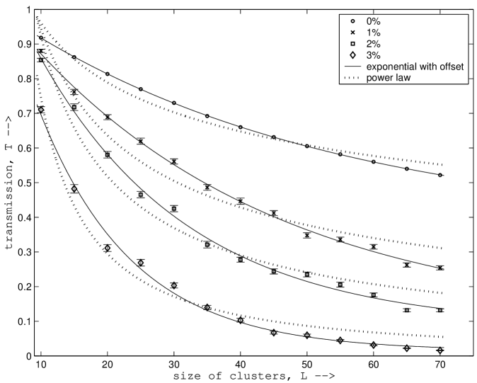
Figure 14: The linear plot of the finite size scaling data of transmission through disordered clusters with diagonally connected leads for low disorder. The dotted lines represent the power-law fits and the solid lines represent exponential fits with finite offsets, both performed on the linear scale as direct, non-linear fits. For this range of disorder, an exponential with a finite offset seems to fit clearly better than a power-law, suggesting a non-zero transmission $T$ even in the thermodynamic limit.

Table 2: Fitting parameters of non-linear fits for diagonal connection at low disorder. Shown in the parentheses are the lower and upper bounds for 95% confidence level.

Disorder	Power law fit: $T=a\cdot L^{-b}$				Exponential fit with offset: $T=a\cdot\mbox{e}^{-bL}+c$
	a	b	$|R|^{2}$	SSE	a	b	c	$|R|^{2}$	SSE
0%	1.85 (1.64, 2.07)	0.28 (0.25, 0.32)	0.96	0.007	0.68 (0.67, 0.68)	0.02 (0.02, 0.02)	0.36 (0.35, 0.37)	1	0.000
1%	3.52 (2.56, 4.47)	0.57 (0.48, 0.66)	0.95	0.024	1.01 (0.97, 1.05)	0.026 (0.02, 0.03)	0.09 (0.02, 0.16)	0.99	0.001
2%	6.31 (4.16, 8.46)	0.83 (0.72, 0.95)	0.96	0.025	1.20 (1.13, 1.28)	0.044 (0.03, 0.05)	0.08 (0.04, 0.12)	0.99	0.002
5%	16.2 (8.47, 24)	1.34 (1.16, 1.52)	0.97	0.015	1.37 (1.22, 1.53)	0.070 (0.06, 0.08)	0.01 (-0.008, 0.03)	0.99	0.003

We have repeated the above procedure for an off-diagonal connection where the input lead is connected at the $5^{th}$ lattice site on the input side and the output lead at the $(L-5)^{th}$ lattice site on the output side ($L$ being the linear size of the clusters). The results for different disorder amounts are plotted in Fig. 15. The central wave vector of the incident wave packet in this simulation is $k_{0}$ = 3.6, keeping all other parameters unchanged. It is clear from the Fig. 15 that the scaling behavior is generally quite similar to that of the diagonal connection; however, the inset appears to indicate that deviations from the power-law fits (straight lines) for the lowest disorder amounts (up to 2%) are much less than the case of the diagonal connection shown in the inset of Fig. 13 for similar values of disorder.

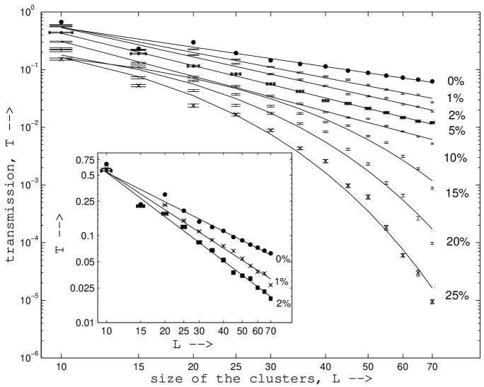
Figure 15: The finite size scaling of transmission through disordered clusters with off-diagonally connected leads (the input lead connected at the $5^{th}$ lattice site on the input side and the output lead is at the $(L-5)^{th}$ lattice site on the output side of the cluster, where $L$ is the linear size of clusters). The main panel shows the log-log plot of $T$ vs $L$ for different disorder amounts, where the solid lines are the best fits performed on the log-log scale similarly to those of the diagonal connection in Fig. 13. The standard errors of the mean are smaller than the size of the symbols except where explicitly plotted. The inset shows the transmission curves only for the lowest disorders with an expanded vertical scale. Every data point is the average over 100 realizations.

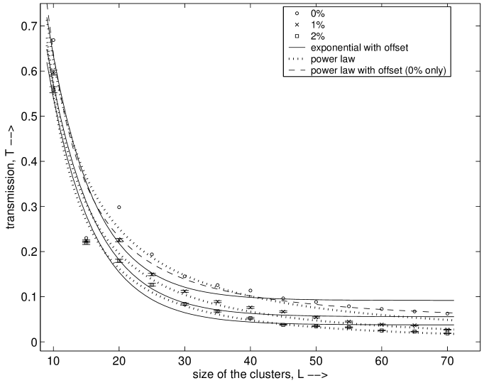
Figure 16: The linear plot of the finite size scaling data of transmission through disordered clusters with off-diagonally connected leads for the lowest disorder values, all performed on the linear scale as direct, non-linear fits. For all three dilutions, 0%, 1%, and 2%, the dotted and solid lines represent power-law fits and exponential fits with offsets, respectively, and in the order of 0%, 1%, and 2% from the top line to the bottom one for each type of fit. From this plot, the power-law fits appear to be better than the exponential with an offset in all cases unlike for the diagonal connection, though a power-law with offset may arguably fit better for the zero-disorder limit.

More closely observing the results from the lowest values of disorder, Fig. 16 shows the data for the off-diagonal connection on the linear scale, together with the results of power-law fit and exponential fit with a finite offset performed as direct, non-linear fits on this scale for 2% or less of disorder. In this case a power-law fits the data significantly better than exponentials with finite offsets, contrary to what we have observed in the case of diagonal connection. For 0% disorder, however, a power-law with finite offset appears to also fit the data well. Thus, it is evident from Fig. 16 and Table 3 that in this particular situation, our data do not support the existence of finite $T$ for non-zero disorder in the thermodynamic limit unlike the case of the diagonal connection.

We emphasize that this study measures transmission in the pseudo-one-dimensional system with a 2D cluster sandwiched between 1D leads. Thus for the global transmission to occur there has to be transmission through the 2D part of the system, requiring extendedness for that part, but boundary perturbations where the chains connect to the cluster may quench the transmission. While boundary effect cannot create global transmission if there is none through the cluster, it could destroy it even if there is transmission through the cluster portion. Though boundary effects must diminish as the cluster size increases, this possibility seems inescapable because of the pseudo-one-dimensional nature of our system. Therefore, the evident lack of global transmission for the case of off-diagonal connection may be due to its quenching of a tenuous extendedness of the cluster due to a boundary perturbation.

Table 3: Fitting parameters of non-linear fits for off-diagonal connection at low disorder. Shown in the parentheses are the lower and upper bounds for 95% confidence level.

Disorder	Power law fit: $T=a\cdot L^{-b}$				Exponential fit with offset: $T=a\cdot\mbox{e}^{-bL}+c$
	a	b	$|R|^{2}$	SSE	a	b	c	$|R|^{2}$	SSE
0%	12.7 (3.6, 21.7)	1.31 (1.04, 1.58)	0.92	0.024	2.33 (0.5, 4.16)	0.15 (0.08, 0.22)	0.09 (0.05, 0.14)	0.90	0.028
1%	20.2 (8.7, 31.7)	1.55 (1.33, 1.77)	0.97	0.009	2.11 (0.91, 3.32)	0.14 (0.09, 0.19)	0.06 (0.02, 0.09)	0.94	0.014
2%	30.9 (17.7, 44.1)	1.75 (1.58, 1.92)	0.99	0.003	2.17 (1.23, 3.11)	0.15 (0.11, 0.19)	0.04 (0.02, 0.06)	0.97	0.007

Summarizing, our work clearly finds exponential localization at least for a dilution of 20% and greater for the energies and connection types treated here. In addition, it also strongly supports the existence of a power-law localized regime at lower disorder as suggested by many in the past. Thus, even though we have not specifically searched for the point of transition between the two localized regimes, there must obviously be a transition between them as we find both at different amounts of disorder. Furthermore, our data are consistent with the existence of an extended state with a finite $T$ in the thermodynamic limit, and thus also a delocalization transition to it, at least for certain energies of the incident particle and for certain types of lead connections (e.g., our diagonal, point-to-point connection), at very low disorder amounts (1% and 2% disorder among our data). Though these findings may not be entirely new individually, we believe that this is the first study in which all three regimes are identified in the same system as the disorder amount is varied.

The issue of the localization length $L_{l}$ must however be discussed since even if the system happens to be exponentially localized in the thermodynamic limit, in order to observe it as such, the localization length of the wave packet must be substantively smaller than the system size. Otherwise, one may observe what appears to be a weaker form of localization (such as power-law) or even an apparently extended state. So it would obviously be useful if we have a theoretical estimate of $L_{l}$ to compare with the system size.

According to the standard approach for an electron transport, $L_{l}\sim\mbox{exp}(k_{f}l_{m})$ where $k_{f}$ is the Fermi wave number of the electron and $l_{m}$ is its mean free path abrahams:79 . Assuming that the mean free path is determined by scattering from the vacant sites, a crude estimate of $\l_{m}$ is the mean separation between vacant sites. Denoting the dilution by $q$ ($0<q<1$), this amounts to $l_{m}\sim 1/q^{1/2}$, or about 10 lattice spacings for 1% dilution and 2 lattice spacings for 20% dilution. The estimation of what to use in place for $k_{f}$ is, however, much more difficult. If we substitute the central wave number for the incident wave packet while it is on the 1D input lead, say, $k_{0}$ = 4.7, into the exponential expression for $L_{l}$ together with the above crude estimates of $l_{m}$, the resulting values come out to be much larger than any conceivable system size one can simulate for almost any amount of dilution. So, according to this scenario, our data should not show exponential localization at all. However, we clearly observe an exponentially localized regime at least for dilutions of about 20% or greater. Thus, it must be that the relevant wave number for the particle as it spreads within the 2D cluster region is rather smaller than $k_{0}$ on the 1D input chain. Since we do not have an independent theoretical estimate of this wave number, the deductive approach outlined above eludes us at this time.

Instead, we have taken a different approach here. Our finite size scaling approach does not rely on any single system size but rather focuses on the trend as it increases. In fact this analysis detects different trends depending on the dilution amount and we can estimate the localization length from the data themselves at least in the clearly observed exponentially localized regime. Indeed, where Tables 1 and 2 indicate the best fits to be the exponential ($a\cdot\mbox{e}^{-bL}$), we can estimate $L_{l}\sim b^{-1}$, interpreting the different system sizes $L$ as analogous to different length scales of observation on a very large system. Table 4 summarizes the simulation estimates of $L_{l}$ made in this way in the regions of disorder where the respective exponential fits are significantly better than other types of fits. From these estimates, it is evident that most of our system sizes at 15% or more dilution are sufficiently large compared with these estimates of $L_{l}$ and thus our results are internally consistent with exponential localization at these amounts of disorder.

Table 4: Estimated values of the localization lengths from $b^{-1}$ in fitting transmission to an exponential without an offset

Disorder	Localization length
	Diagonal	Off-diagonal
	connection	connection
15%	-	12.2
20%	8.3	8.6
25%	6.4	6.5
30%	4.7	-

We could, in addition, also force fits to an exponential without an offset for smaller dilution where other fits such as power-laws or those with a non-zero offset are actually significantly better than the pure exponential. This is because, if in fact the state were exponentially localized but it happens to fit better either a power-law or an exponential with a finite offset because of the small system size, then one might expect a forced, pure-exponential fit to reveal a hint of the localization length that is larger than the system size. When this is done for the diagonal connection, the resulting estimates of $L_{l}$ vary as 10 (for 15% disorder), 10 (10%), 16 (5%), 32 (2%), 50 (1%), and 111 (0%), while the off-diagonal connection data of Fig. 15 vary as 17 (10%), 18 (5%), 20 (2%), 22 (1%), and 30 (0%). Thus, the estimates for the diagonal connection do not agree with such expectation, or, in other words, the system size limitation does not seem to be a factor in the apparent existence of the extended regime, at least for 1% and 2% disorder. Those for the off-diagonal connection do not agree with the expectation as well for all values of dilution used, thus in this case, the power-law localization appears to be genuine and not the artifact of the system size limitation.

V Summary and Conclusion

In this work we have developed a tool to visualize the propagation of a Gaussian wave packet through a 2D cluster connected with 1D leads under various conditions. We applied this dynamical method to study the behavior of a quantum particle in completely ordered as well as disordered quantum percolation systems realized both on the square and triangular lattices. The method is very useful to study the scattering of a quantum particle by potential barriers. Since we can visualize and track the wave packet in real time, we can investigate how a particle propagates through a disordered system and how it is trapped inside the cluster.

For completely ordered systems, transmission is dominated by the interference effect. It also depends on the way the leads are connected to the cluster in complex ways. Transmission is generally high for the diagonally connected leads except for those wave vectors for which destructive interference gives rise to close-to-zero transmission (reflection resonances). For the busbar type connection, generally low transmission is observed because of large interference effects of the wave packet with the edge on the input side of the cluster, but with significant transmission peaks (resonances) at certain energies.

An important application of this method may be to probe the existence or absence of a localized-delocalized transition in the two-dimensional, disordered system. Our finite-size scaling results imply that there exists a phase transition between a power-law localization and an exponential localization regimes. In addition to this, our study further suggests that there may exist delocalized states at very low disorder, consistent with the proposition that delocalization transition exists in the 2D disordered quantum percolation system, adding to the increasing literature on this still controversial issue. Of course, since the present work is based on specifically constructed wave packets and is based on relatively small and limited types of geometry, further studies are called for to unequivocally determine the answers to these issues. In particular, direct solutions of the Schrödinger equation along the lines of Daboul et aldaboul:00 are desirable, and are being investigated.islam:07

References

- (1) E. Cuansing and Hisao Nakanishi, Phys. Rev. E, 70, 066142 (2004)
- (2) C. M. Soukoulis, E. N. Economou, and G. S. Grest, Phys. Rev. B, 36, 8649 (1987)
- (3) Th. Koslowski and W. von Niessen, Phys. Rev. B, 44, 9926 (1991)
- (4) R. Berkovits and Y. Avishai, Phys. Rev. B, 53, R16125 (1996)
- (5) E. Abrahams and P.W. Anderson and D.C. Licciardello and T.V. Ramakrishnan, Phys. Rev. Lett., 42, 673 (1979)
- (6) However, a recent work of N. Goldenfeld and R. Haydock, Phys. Rev. B, 73, 045118 (2006) concludes that a transition between two localized states exists for the 2D Anderson model.
- (7) G.J.Dolan and D.D Osheroff, Phys. Rev. Lett., 43, 721 (1979)
- (8) D.J. Bishop and D.C. Tsui and R.C Dynes, Phys. Rev. Lett., 44, 1153 (1980)
- (9) M.J. Uren and R.A. Davies and M. Papper, J. Phys. C, 13, L985 (1980)
- (10) E. Abrahams and S.V. Kravchenko and M.P. Sarachik, Rev. Mod. Phys., 73, 251, (2001)
- (11) D. Daboul and I. Chang and A. Aharony, Eur. Phys. J, B 16, 303 (2000)
- (12) T. Odagaki and K. C. Chang, Phys. Rev. B, 30, 1612 (1984)
- (13) V. Srivastava and M. Chaturvedi, Phys. Rev. B, 30, 2238 (1984)
- (14) M. Letz and K. Ziegler, Phil. Mag. B 79, 491 (1999)
- (15) H. N. Nazareno, P. E. de Brito and E. S. Rodrigues, Phys. Rev. B 66, 012205 (2002)
- (16) A. Eilmes, R. A. Römer and M. Schreiber, Physica B 296, 46 (2001)
- (17) G. Hałdaś and A. Kolek and A. W. Stadler, Phys. Status Solidi B, 230, 249 (2002)
- (18) A. Bunde and J. W. Kantelhardt and L. Schweitzer, Ann. Phys. (Leipzig), 7, 372 (1998)
- (19) C. M. Soukoulis and G. S. Grest, Phys. Rev. B, 44, 4685 (1991)
- (20) A. Mookerjee and I. Dasgupta and T. Saha, Int. J. Mod. Phys. B, 9, 2989 (1995)
- (21) M. Inui and S. A. Trugman and E. Abrahams, Phys. Rev. B, 49, 3190 (1994)
- (22) N.J. Giordano and H. Nakanishi, Computational Physics, Pearson Prentice Hall, Second edition, pages 334-335 (2005)
- (23) E. Cuansing and H. Nakanishi (unpublished), Md. F. Islam and H. Nakanishi (unpublished).