NICMOS Observations of Shocked H₂ in Orion¹

Abstract

HST NICMOS narrowband images of the shocked molecular hydrogen emission in OMC-1 are analyzed to reveal new information on the BN/KL outflow. The outstanding morphological feature of this region is the array of molecular hydrogen “fingers” emanating from the general vicinity of IRc2 and the presence of several Herbig-Haro objects. The NICMOS images appear to resolve individual shock fronts. This work is a more quantitative and detailed analysis of our data from a previous paper Schultz et al..

Line strengths for the H₂ 1–0 S(4) plus 2–1 S(6) lines at 1.89 µm are estimated from measurements with the Paschen $\alpha$ continuum filter F190N at 1.90 µm, and continuum measurements at 1.66 and 2.15 µm. We compare the observed H₂ line strengths and ratios of the 1.89 µm and 2.12 µm 1–0 S(1) lines with models for molecular cloud shock waves. Most of the data cannot be fit by J-shocks, but are well matched by C-shocks with shock velocities in the range of 20–45 km s^-1 and preshock densities of $10^{4}-10^{6}$ cm^-3, similiar to values obtained in larger beam studies which averaged over many shocks. There is also some evidence that shocks with higher densities have lower velocities.

1 Introduction

At 450 pc, the Orion molecular cloud is the nearest and best-studied region of massive star formation. The Trapezium stars, formed within Orion Molecular Cloud 1, have cleared a cavity at the near edge of the cloud. The visible Orion Nebula is the thin layer of photo-ionized gas on the cavity’s surface facing the observer. Behind M42, and further from the observer, is a photodissociation region (PDR) also excited by the Trapezium. The BN/KL region lies still deeper in the cloud, beyond both the ionized gas and the PDR. This region contains embedded sources with one or more associated outflows; the total luminosity of this region approaches $\sim 10^{5}L_{\sun}$ (Genzel & Stutzki, 1989). The mid-infrared source IRc2 had long been thought to be the origin of these outflows; but Dougados et al. (1993) resolved IRc2 into four sources, raising the possibility that none of them is sufficiently powerful to drive the observed outflows. Menten & Reid (1995) suggested that the origin may be closer to the infrared source “n” (Lonsdale et al., 1982), located $\approx$ 5″ SW of IRc2. Greenhill et al. (2004) detected extended emission from source n at wavelengths out to 22 µm, but estimate a luminosity of only 2000 $L_{\sun}$. They also resolved IRc2 into $\sim 5$ knots and suggested that these sources together with radio source I (Churchwell et al., 1987) comprise at least part of the core of a high density star forming cluster.

The most striking of the molecular hydrogen outflows is an $\sim 3^{\prime}$ (0.4 pc) sized, butterfly-shaped region of H₂ emission, centered to the north of BN, which exhibits line ratios typical of shock excitation (Beckwith et al., 1978). From O I emission, Axon & Taylor (1984) identified a number of optical HH objects in this vicinity. Taylor et al. (1984) discovered peculiar linear H₂ structures in the outflow. Allen & Burton (1993, hereafter AB) showed that these H₂ “fingers” and all the associated optical HH objects at the far northern end of the outflow (approximately 120″ from BN) terminated in knots of Fe II emission. Stolovy et al. (1998) found additional H₂ fingers within 30″ of BN. Schultz et al. , found that only 2 of the 15 inner fingers seen by Stolovy et al. (1998) had bow shocks capped by Fe II emission, suggesting a lower excitation than in the outer fingers seen by AB.

From offsets between the peak H₂ emission and the peak H₂ velocity, Gustafsson et al. (2003) suggested that the H₂ emission arises in part from outflows from protostars within dense clumps of gas. In contrast, based on proper motion studies of optical features, Doi et al. (2002) found that both finger systems could have been created by an explosive event close to the IRc2-BN complex which took place approximately 1000 years ago. Interestingly, Rodríguez et al. (2005) and Gómez et al. (2005) suggested that BN and sources I and n were originally part of a multiple massive stellar system that disintegrated about 500 years ago. Explanations for the unique system of fingers have focused on two theories. AB originally suggested that they are “bullets”—ejected clumps leaving a wake of shocked material behind them. However, the observed morphology of the H₂ emission is inconsistent with models for bullets (Stone & Norman, 1992, Klein et al., 1994, Xu & Stone, 1995, Jones et al., 1996). These models predict that rapidly moving clumps are fragmented and also predict that the tails should be pointing away from the ejection source, which is not seen. Stone et al. (1995) suggested the features are produced when a faster wind collides with a slower, older outflow. Rayleigh-Taylor instabilities from the collision form the clumps in situ, moving at the speed of the older outflow. The observed fingers then condense behind the slowly moving clumps. This is similar to the mechanism thought to have produced the cometary knots in the Helix Nebula (O’Dell & Handron, 1996). One prediction of this model is that a region of clumpy H₂ emission will form behind (i.e. upstream of) the bullets. McCaughrean & Mac Low (1997) claimed to have found this clumpy emission in the central region of the H₂ outflow. However, our previous work (Paper, 1) and that of (Stolovy et al., 1998) shows that much of this “clumpy” H₂ emission is resolved into more discrete objects, some resembling additional fingers. The remaining, unresolved clumpy emission is often mixed with the inner fingers.

Here we discuss the interpretation of our previously published NICMOS infrared images of a 90″ wide region centered on BN/KL, focusing on the structure of the H₂ emission. Examination of the F190N images, originally obtained for subtracting continuum from the P$\alpha$ 1.87 µm images (Paper, 1), suggested that in many regions there was a strong correlation with the H₂ 1–0 S(1) 2.12 µm continuum-subtracted images. In fact, the F190N filter bandpass includes both the H₂ 1-0 S(4) and the 2-1 S(6) lines at 1.89 µm. This H₂ emission is likely produced in shocks (Gautier et al., 1976). H₂ emission can also be produced through UV fluorescence, but larger beam studies of multiple H₂ transitions by Usuda et al. (1996), Rosenthal et al. (2000), and many others have shown that the measured line ratios in this region are consistent only with thermal excitation and not UV fluorescence. In this paper, we focus on the finger-like structures and the HH objects. Some of these objects have optical counterparts, which places constraints on their position within the cloud/nebula interface. In §2 we discuss the observations and data reduction. In §3 we compare the observed H₂ line brightnesses with several classes of shock models in order to determine shock types, shock velocities, and gas densities. In §4 we discuss the morphology of, and emission from, many of the more distinct, brighter features seen in our images.

2 Observations

Observations were made of H₂ 1–0 S(1) 2.12 µm and 1–0 S(4) plus 2–1 S(6) 1.89 µm in the 1% bandpass NICMOS filters. The initial reduction of the NICMOS data was described in detail in Paper 1 and generally followed standard procedures. Photometry was then performed on the reduced data from Paper 1 using the IRAF (Tody, 1993) task polyphot, in which the average brightness is estimated inside a user-defined polygonal aperture. The apertures were designed to closely follow the outline of each object we identified. Sky subtraction was not performed with the polyphot task, but separately using a region or regions far from areas of obvious emission. Regions selected for photometry are shown in Figure 1. Knot designations, except for HH 208, utilize the source identification scheme of O’Dell & Wen (1994). Knot identifications for HH 208 are shown in Figure 11. The features were selected for being distinct and fairly bright, having detectable 1.66 µm and 2.15 µm continuum emission, and 2.12 µm line emission. Knot U was also included even though it had no detectable 1.66 µm continuum. The resulting photometry is listed in Columns 2-5 of Table 1. The formal statistical errors are such that the signal-to-noise ratios of all the measurements in Table 1 exceed 25 except for three: i) the 1.66 µm measurement of 128–248 (S/N $=4$), ii) the 1.66 µm measurement of HH 208U (not detected), and iii) the 2.15 µm measurement of HH 208U (S/N=15).

There are no continuum observations for the H₂ 1.892 µm 1–0 S(4) plus 2–1 S(6) images. However, we did observe continua at 1.66 and 2.15 µm, intended as continua for the Fe II and 1–0 S(1) lines respectively. The 1.89 µm continuum has been estimated from these continuum measurements by linearly interpolating between the 1.66 µm and 2.15 µm photometric measurements. The continuum interpolation approach was checked by applying the same technique to nine regions with no 2.12 µm H₂ emission. In these test regions, the interpolated continuum value was on average $99\pm 3$% of the value actually measured in the F190N filter, confirming that this is a reasonable approach. As an example of the interpolation, the brightnesses for 128–248, with the estimated continuum is shown in Figure 2.

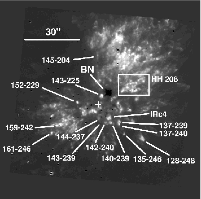
Figure 1: H₂ 1–0 S(1) image of the Orion region with the selected features labelled. North is up and east is to the left. BN is located at $05^{\rm h}35^{\rm m}14.^{\rm s}12,-05^{\arcdeg}22^{\prime}23.^{\prime\prime}2$ (J2000) and the location of IRc2 is noted by a cross.

Table 1: H₂ Photometry and Results

		Measured Line plus Continuum					Extinction Corrected H2 Brightnesses
Position		1.66 µm	1.90 µm	2.12µm	2.15 µm		$A_{2.12\mu{\rm m}}$	$A_{V}$	1.89 µm	2.12 µm
		[$10^{-3}$ ergs s-1 cm-2 sr-1]					(mag)	(mag)	[$10^{-3}$ ergs s-1 cm-2 sr-1]
HH 208A		0.31	1.14	2.63	1.37		0.6	4.5	0.70	2.33
HH 208B		1.15	3.90	11.1	3.87		0.6	4.5	2.94	13.0
HH 208D		0.85	2.55	9.96	1.96		0.6	4.5	2.31	14.0
HH 208E		0.72	2.28	7.96	1.84		0.6	4.5	2.03	10.8
HH 208F		0.25	1.88	7.96	1.72		0.6	4.5	1.90	11.0
HH 208J		0.54	2.28	9.49	1.84		0.6	4.5	2.24	13.5
HH 208N		3.31	4.10	9.53	3.09		0.6	4.5	1.50	11.1
HH 208P		0.02	1.68	7.66	1.01		0.6	4.5	2.38	11.7
HH 208R		1.85	2.55	9.15	1.60		0.6	4.5	1.45	13.0
HH 208U		0.0	0.42	1.82	0.21		0.6	4.5	0.63	2.82
128–248		0.02	1.28	6.34	1.01		1.0	8	2.57	13.6
135–246		0.33	1.08	3.20	0.71		0.6	4.5	1.10	4.38
137–239		0.34	1.48	7.02	0.95		1.0	8	2.61	15.4
137–240		0.33	1.54	7.32	1.01		1.0	8	2.76	16.0
140–239		0.56	2.48	9.74	2.37		0.6	4.5	2.16	13.0
142–240		0.54	1.81	5.28	1.72		0.6	4.5	1.43	6.34
143–225		0.85	3.90	12.6	5.15		1.0	8	3.80	32.4
143–239		0.51	0.94	1.49	0.83		0.6	4.5	0.54	1.19
144–237		0.54	1.20	3.74	0.89		0.6	4.5	0.96	4.98
145–204		0.18	1.01	4.17	1.13		1.0	8	1.31	7.83
152–229		0.30	2.15	7.83	3.15		0.6	4.5	1.16	8.51
159–242		0.69	3.22	12.0	1.84		0.6	4.5	3.88	17.8
161–246		0.85	2.48	7.70	1.54		0.6	4.5	2.52	10.8

Figure 2: The estimation of H₂ line brightnesses for 128–248. The boxes show the measured photometric points; errors are smaller than the boxes. The X’s show the estimated continuum at the wavelengths of the H₂ lines. The 2.12 µm continuum was set equal to the 2.15 µm measurement.

The extinction corrections in this region are complex, and vary depending upon the distribution of intervening dust, which lies not only within the molecular cloud but also in the PDR and in foreground material. Extinction estimates are also complicated by reflection off the back side of the nebula. Most of our objects, including two fingers and several more compact structures, have some associated Fe II (1.64 µm) emission (Schultz et al., 2007). For these objects, the 2.12 µm extinction can be estimated from the results of Chrysostomou et al. (1997), who used measurements of the Fe II 1.257 and 1.644 µm transitions, and the extinction curve of Cardelli et al. (1989), to obtain the extinction values of 0.6 shown in column 6 of Table 1. For five regions, no Fe II emission is seen, possibly because of larger extinction. The extinction for these particular objects hasn’t been estimated by Chrysostomou et al. (1997), or others. The best references are large beam extinction studies of the H₂ Peak 1 source. The largest and most recent such study is that of Rosenthal et al. (2000), based on the ISO measurement of 56 H₂ transitions covering wavelengths of 2-17 µm. They find A${}_{K}=1.0\pm 0.1$, a value we adopt here for 128–248, 137–239, 137–240, 143–225, and 145–204. For wavelengths other than 2.12 µm, the brightnesses have been extinction corrected using A${}_{\lambda}=$ A${}_{2.12}\{{{\lambda}\over{2.12}}\}^{-1.61}$ (Cardelli et al., 1989), who also found that the shape of the extinction curve in the IR is independent of the value assumed for R_V. Usage of different plausible extinction corrections, within the uncertainties, does not appreciably alter our conclusions. For reference, we show in column 7 the approximate visual extinctions, A${}_{V}=4.5$ and A${}_{V}\sim 8$, based upon R${}_{V}=$A_V/E${}_{(B-V)}=3.1$, and Cardelli et al. (1989). The final 1.89 µm H₂ line-to-continuum ratios range from 0.25 to 1.1, with a median of 0.7.

3 Shocked Emission Features: Line Ratio Analysis

Early shock models of the Orion outflow invoked planar C-type shock models to explain the emission from species such as H₂ and CO (e.g. Draine & Roberge, 1982, Chernoff et al., 1982). C-type or “continuous” shocks occur at relatively low shock speeds ($V_{shock}\lesssim 50$ km s^-1) in the presence of magnetic fields. A low ionization fraction allows ionized gas to cushion the shock in the neutral gas, limiting the neutral gas temperature to less than several thousand Kelvin and preventing significant dissociation. J-type or “jump” shocks generally occur at relatively high shock speeds ($V_{shock}\gtrsim 50$ km s^-1) and usually dissociate molecular gas in the high temperature ($T\sim 10^{4}-10^{5}$ K) post-shock region. Molecules reform in the cooling post-shock gas at T$\sim$500 K. For pre-shock densities $\gtrsim 10^{5}\,\rm cm^{-3}$, H₂ line ratios produced in the reforming molecular gas may reach values higher than thermal values since H₂ reforms in excited states, leading to a non-thermal cascade through rovibrational states (Hollenbach & McKee, 1989).

Observations of shocked H₂O emission in Orion (e.g. Harwit et al., 1998) seem to confirm the general picture that C-type shocks are responsible for the molecular emission in the outflow. These studies converge on preshock conditions $n(\rm H_{2})\sim 10^{5}\,\rm cm^{-3}$ and $V_{shock}\sim 35$ km s^-1 (e.g. Chernoff et al., 1982). It should be noted, however, that these studies fit data collected from a beam area covering an entire outflow lobe ($\sim 1\arcmin\sim 0.1$ pc at Orion). Images of the shocked emission on sub-arcsecond scales (AB, Stolovy et al., 1998) show many emission features, each of which presumably has its own shock conditions. What is unique about the NICMOS observations of the inner region is that the 0.″2 ($\sim 1.4\times 10^{15}\,\rm cm$) resolution allows the isolation of individual shock fronts on the length scales expected for such shocks. These scales are expected to be $\sim 10^{15}\,\rm cm$, depending on the preshock density but with only a weak dependence on the shock velocity (Kaufman & Neufeld, 1996). This means that our deduced shock parameters are more likely to represent the local physical conditions, rather than an average over a number of shocks.

H₂ adaptive optics observations of the ambient molecular cloud to the south-east of BN/KL have been carried out with $0.^{\prime\prime}15$ angular resolution (Vannier et al., 2001; Kristensen et al., 2003). The observed H₂ 1-0 S(1) brightness is well matched by C-shock models with shock velocities of 30 km s^-1 and pre-shock densities of $10^{6}\,\rm cm^{-3}$, but the same models fall short of matching the 2-1 S(1) brightness by a factor $\sim$2 (Vannier et al., 2001). Higher shock velocity models improve the 2-1 S(1) brightness prediction, but provide a worse fit to the 1-0 S(1) brightness. J-shock models produce the observed 2-1 S(1)/1-0 S(1) brightness ratio but have trouble reproducing the individual line brightnesses. Pineau des Forêts & Flower (2001) suggested that non-stationary C-shocks can reproduce the high brightness and the large observed 2-1 S(1)/1-0 S(1) brightness ratios. However, non-stationary C-shocks have difficulty accounting for the proper motion velocity measurements of Doi et al. (2002), who found that over the velocity range of 20 – 400 km s^-1, different emission lines from the same object have similar velocities. From comparison with the higher excitation H₂ 2-1 S(1) line, Kristensen et al. (2003) found H₂ clumps to have abrupt, south-facing edges exhibiting high excitation temperatures. Even C-shocks propagating into high density material can’t account for the excitation temperature maxima and the line fluxes. This led Kristensen et al. (2003) to suggest that J-shocks propagating into material with a pre-shock density $\geq 10^{6}\,\rm cm^{-3}$, plus an additional contribution from photo-dissociated material, are required to explain these measurements. Emission from bow-shaped shock fronts (Smith et al., 1991), in which both C-shocks and J-shocks are responsible for the overall emission, may also help explain these observed brightnesses and line ratios.

For our study, we use the ratio of the H₂ line fluxes at 2.12 and 1.89 µm as a diagnostic of conditions in the emitting gas. The Camera 3 F190N filter transmission plot was examined to determine the relative throughput of the 1-0 S(4) (1.892 µm) and 2-1 S(6) (1.8947 µm) rovibrational transitions. From the transmission plot, we estimate the NICMOS filter transmissions at the H₂ wavelengths to be 64% and 98% respectively. Hence, we compare the measurements with model predictions for $0.64\times$B[1-0 S(4)]$+0.98\times$B[2-1 S(6)]. All three transitions require gas temperatures in excess of 1000 K in order to produce significant emission. Such high temperatures imply that shock excitation is responsible for the H₂ emission. A difficulty with interpreting the 2.12 and 1.89 µm lines is that the transitions are relatively close together in excitation: the upper state of the S(1) line is at 6956K, and that of the S(4) and S(6) lines are at 9286K and 16880K, which can be a rather small baseline to fit.

In an effort to characterize the shocked H₂ emission, we have compared our observed line brightnesses and line ratios with standard models of shock emission: the C-shock model of Kaufman & Neufeld (1996) and the J-shock model of Hollenbach & McKee (1989). We first consider 128–248, a well-isolated source for which we obtain the highest signal-to-noise ratio at 1.89 and 2.12 µm. Because the large beam studies suggest shocked gas with densities near $10^{5}\,\rm cm^{-3}$, we computed the brightnesses of the 1-0 S(1) and $0.64\times$B[1-0 S(4)]$+0.98\times$B[2-1 S(6)] transitions in C-shocks with preshock densities of $10^{4},\,10^{5}$ and $10^{6}\,\rm cm^{-3}$ and shock speeds up to 50 km s^-1; and in J-shocks with preshock densities of $10^{5},\,10^{6}$ and $10^{7}\,\rm cm^{-3}$ and shock speeds up to 100 km s^-1. In line with current practice, the models assume a) a planar shock, b) a magnetic field perpendicular to the direction of propagation of the shock, and c) the magnetic field strength in microgauss equals the square root of the density in cm^-3 (Troland & Heiles, 1986). The precise structure of the C-shocks depends on the field strength, as well as the ionization fraction, the grain size distribution, and the details of gas cooling. We have previously explored the effects of varying these parameters on shock structure (Kaufman & Neufeld, 1996). We find that while the precise value of shock velocity and density determined from a line ratio may vary from those presented here, the range of intensities and line ratios possible in C-shock models is essentially limited by the temperature at which H₂ dissociates. Thus our conclusion that C-shocks can explain the emission in most of the observed features is robust even if the precise shock parameters are different from those we have assumed.

At this assumed magnetic field strength, low velocity shocks are C-shocks and not the lower magnetic field strength, non-dissociative, molecular J-shocks discussed by Wilgenbus et al. (2000). Typically, molecular J-shocks produce a factor of 10-1000 times fainter H₂ emission in the lines discussed here than C-shocks (Wilgenbus et al., 2000). Since these line fluxes would be undetectable, we have not included non-dissociative, molecular J-shocks in our grid of models. Higher velocity shocks would be dissociative J-shocks, which we do consider. C-shocks are also known to be unstable to the Wardle instability (Wardle, 1990) arising from perturbations in the magnetic field direction, an effect which is not taken into account in the steady-state C-shock models presented here. The effects of this instability on the strengths of H₂ emission lines has been explored by Mac Low & Smith (1997) and Neufeld & Stone (1997). Both studies reached the conclusion that, for shocks over the range of densities and shock velocities we consider (i.e. shocks for which H₂ is the dominant coolant), the instability has little effect on the predicted intensities of H₂ lines. Thus our steady-state models should be sufficient for modeling the emission presented here. Clearly, changing the assumptions in the shock models - bowshocks instead of plane-parallel shocks, stronger or weaker magnetic fields, a different orientation of the magnetic field with respect to the shock, etc. - will result in different predictions for the H₂ line strengths, perhaps resulting in better (or worse) agreement with our data. A complete exploration of this parameter space is beyond the scope of this paper, but we can show that for some commonly-assumed magnetic field properties, plane-parallel C-shock models provide a reasonable fit to the data, while plane-parallel J-shock models generally do not.

The predicted brightness ratio {$0.64\times$B[1-0 S(4)]$+0.98\times$B[2-1 S(6)]}/B[1-0 S(1)] from each model calculation is shown in Figure 3 as a function of shock velocity. Also shown is the measured ratio, 0.19, for 128–248. The line ratio is consistent with either C- or J-shocks. However, the line ratio and brightness from this feature is best fit by a C-shock model with velocity 36 km s^-1 and preshock density of $6\times 10^{4}\,\rm cm^{-3}$. The brightnesses, line ratio, and model predictions for 128–248 are listed in Table 2. The model values are well within the systematic measurement uncertainties. J-shocks produce absolute intensities which are too low to match the observed values.

Table 2: Observed Brightnesses and Model Fit for 128–248

	$0.64\times$B[1-0 S(4)]$+0.98\times$B[2-1 S(6)]	B[1-0 S(1)]	$0.64\times$B[1-0 S(4)]$+0.98\times$B[2-1 S(6)]
	[$\rm erg\,s^{-1}\,cm^{-2}\,sr^{-1}$]		/B[1-0 S(1)]
Observed	$2.57\times 10^{-3}$	$1.36\times 10^{-2}$	0.190
Model	$2.60\times 10^{-3}$	$1.31\times 10^{-2}$	0.198

Figure 3: Predicted {$0.64\times$B[1-0 S(4)]$+0.98\times$B[2-1 S(6)]}/1-0 S(1) line ratio from C-shock and J-shock models with magnetic fields oriented perpendicular to the shock propagation direction and strengths in microgauss equal to the square root of the density in cm^-3 (Troland & Heiles, 1986). Results are shown for C-shock models with $n(\rm H_{2})=10^{4},\,10^{5}$ and $10^{6}\,\rm cm^{-3}$ and $V_{shock}=15-50$ km s^-1, and J-shock models with $n(\rm H_{2})=10^{5},\,10^{6}$ and $10^{7}\,\rm cm^{-3}$ and $V_{shock}=30-100$ km s^-1. Also shown is the measured value of the line ratio for the Orion feature 128–248 (horizontal solid line), with the statistical uncertainty in the ratio indicated by the dashed lines.

The extinction-corrected line flux ratio for each of ten locations in HH 208 and thirteen other features is plotted versus their 2.12 µm H₂ line brightness in Figure 4. The shock model curves are overlain. Within the systematic measurement uncertainties, all but one of the observed line ratios are consistent with C-shocks having preshock densities $10^{4}\,-\,10^{6}\,\rm cm^{-3}$ and shock velocities of 20 to 45 km s^-1. The narrow range of shock velocities is not surprising. Slower C-shocks produce much weaker H₂ emission and would not have been detected. Faster C-shocks break down into J-shocks, again with much fainter H₂ emission because the H₂ is dissociated. The consistency with larger beam studies does suggest that these studies yield reasonable average shock parameters. Table 3 lists shock velocities and pre-shock densities for all the objects. These values were estimated by interpolating within the grid of calculated C-shock models at densities of $10^{4}$, $10^{5}$, $10^{6}$ and shock velocities of 20, 25, 30, 35, and 40  km s^-1, whose curves are plotted in Figure 4. Extrapolations for those objects just outside the grid were made using a few additional models with shock velocities of 45  km s^-1. Two objects - 143–239 and HH208A - are clearly outside the C-shock grid.

Examination of Figure 4 suggests that higher shock velocities may be correlated with lower pre-shock densities. A variety of statistical tests show that this correlation is significant at the 3-4$\sigma$ level. The log of the pre-shock density falls by $\sim 0.6$ for each shock velocity increase of 10  km s^-1. In order to search for structure such as the “hot edges” found by Kristensen et al. (2003), we have constructed and examined images of the line flux ratio for all twenty three of the features included in Figure 4. We find no significant structure in the ratio images except for 145–204 and 159–242, where there is a peak in the line ratio offset by 1-2″ from the peak H₂ 1–0 S(1) emission.

Figure 4: The log of the {$0.64\times$B[1–0 S(4)]$+0.98\times$B[2–1 S(6)]}/[1–0 S(1)] brightness ratio plotted versus the log of the 1–0 S(1) brightness. Measured values for each of the shocked fingers with both 1.89 µm and 2.12 µm emission are given by the pentagons. The symbols for the HH 208 positions are hollow. The error bars in the data are smaller than the data symbols. A trend arrow indicating the direction and magnitude of the change in the observed ratio and brightness if the 2.12 µm extinction was increased from 0.6 to 2.4 mag, is given by the solid arrow. The symbol outlined by a box represents source 128–248. Model curves are shown for C-shocks (solid curves, labeled with log[$n(\rm H_{2})$/cm${}^{-3}]=$4, 5, 6 and shock velocity of 25–40 km s^-1) and J-shocks (solid, dotted, and dashed curves, labeled with log[density/cm${}^{-3}]=$5, 6, 7 and shock velocity of 30–100 km s^-1). For both C- and J-shocks, the magnetic fields are oriented perpendicular to the shock propagation direction with strengths in microgauss equal to the square root of the density in cm^-3 (Troland & Heiles, 1986). Factors contributing to uncertainties in the model predictions are discussed in §3.

Table 3: Estimated C-Shock Velocities and Pre-Shock Densities

Position	$v_{S}$ (km s-1)	log$[n_{\rm H_{2}}({\rm cm}^{-3})]$
HH 208B	42	4.5
HH 208D	32	4.8
HH 208E	36	4.5
HH 208F	33	4.6
HH 208J	32	4.8
HH 208N	27	5.2
HH 208P	40	4.5
HH 208R	26	5.5
HH 208U	42	4.0
128–248	36	4.8
135–246	45	4.0
137–239	32	4.8
137–240	33	4.8
140–239	32	4.7
142–240	42	4.3
143–225	27	5.8
144–237	38	4.3
145–204	33	4.6
152–229	27	5.0
159–242	41	4.5
161–246	42	4.4

4 Results and Discussion

In this section, we outline the morphological and emission characteristics of the H₂ features. We categorize the features into fingers - structures which either exhibit a clear bow shock morphology or features we believe to be bow shocks approaching us at a low angle - and knots - mostly including a variety of clumps in HH 208.

4.1 Fingers

The array of inner fingers which comprises the butterfly-shaped H₂ emission first found by Beckwith et al. (1978), extends over a 90″ broad region. Most of the northern H₂ fingers (AB) are outside of our field to the north, but there are additional fingers to the south, east of the Trapezium (McCaughrean & Mac Low, 1997). The velocity measurements of Chrysostomou et al. (1997) found that in addition to strong, broad H₂ emission over the entire source, there are high velocity components confined to discrete condensations. The high velocity components are ascribed to additional ‘bullets’ similar to those imaged in the northern fingers by AB. At our higher angular resolution, the morphology of the inner fingers (Finger 1) is quite varied. Some of the objects are revealed to be bright, well-defined bow shocks; others do not display distinct bows of any kind. Most of the objects are found to have complex structure, with what appear to be internal shocks.

4.1.1 128–248 and 135–246

128–248 is a bright, well-defined bow-shock in the southwestern portion of the finger array. Because it is so bright, and well-separated from the main array by dark dust lanes, 128–248 is an excellent candidate for many studies. Schultz & Burton (2007) found a FWHM of 30 km s^-1, while Chrysostomou et al. (1997, their object 10) found it to have a FWZI of 150 km s^-1 . Schultz & Burton (2007) and Gustafsson et al. (2003, their region 11) found that its line profile has no secondary line peaks, which is suprising for a bow shock, and almost unique among the inner fingers. From its peak velocity of 0 km s^-1, Gustafsson et al. (2003) concluded that 128–248 is moving in the plane of the sky, but were unable to determine in what direction. The H₂ emission morphology is shown in Figure 5 - a classic bow-shock shape which appears to be moving to the southwest. From the line fluxes, we deduce a shock velocity and pre-shock density of 36 km s^-1 and $10^{4.8}$ cm^-3 for 128–248.

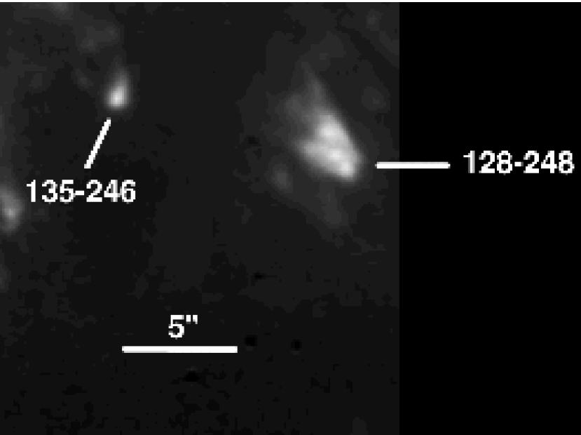
Figure 5: H₂ 1–0 S(1) image of 128–248 and 135–246. North is up and east is to the left. The maximum brightness is 8.9$\times 10^{-3}$ ergs s^-1cm^-2sr^-1.

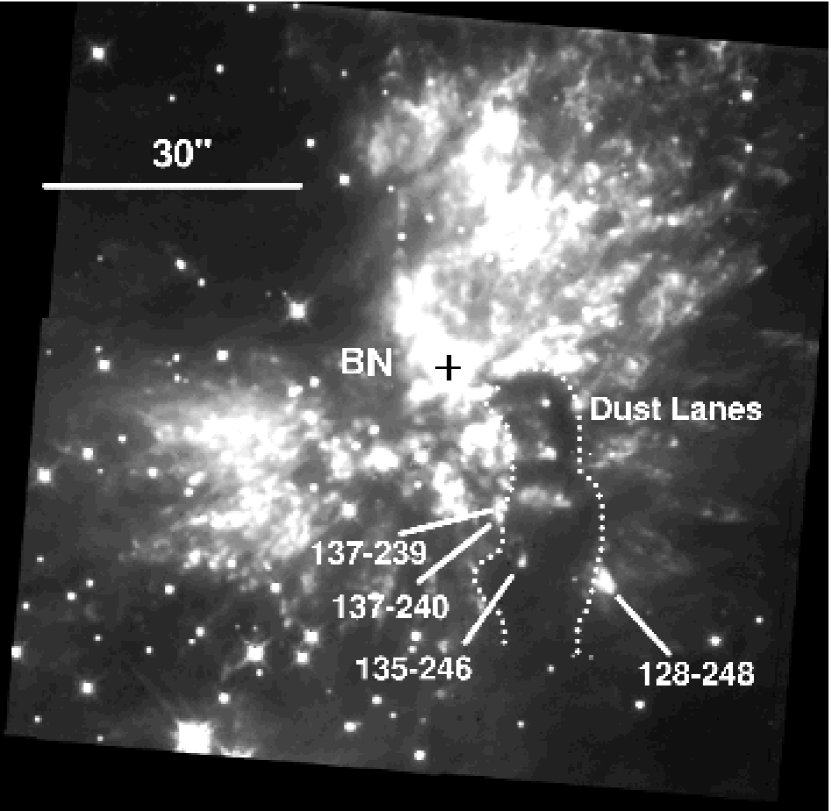
Figure 6: 2.12 µm continuum plus H₂ 1–0 S(1) line map showing the locations of 128–248, 135–246, 137–239, and 137–240 relative to the dust lanes and BN. The Trapezium is off the bottom of the image. North is up and east is to the left.

135–246 is a bright bow shock at the end of a faint finger emerging from a extended continuum “tail” of IRc4 (cf. Figure 1). It is prominent in H₂ 1-0 S(1), Fe II (Schultz et al., 2007), and the F190N and F215N continuum bandpasses. The object also appears in O I and possibly in S II emission (Schultz et al., 2007). Our H₂ image is shown in Figure 5 - from the line ratios we deduce a shock velocity and pre-shock density of 45 km s^-1 and $10^{4.0}$ cm^-3. The northeast boundary of the bright tip of the 135–246 bow shock is very sharp. We suggest this is probably due to the emergence of the finger from behind a region of high extinction: Figure 6 shows that the southwestern extent of the H₂ finger is partially obscured by the same dark, curving dust lanes which are near 128-248 and the region south of BN.

4.1.2 137–239, 137–240, and 140–239

The H₂ emission from 137–239, 137–240, and 140–239 is shown in Figure 7. From our analysis, 137–239, 137–240, and 140–239 are all fit by shock velocities of 32 to 33 km s^-1 and pre-shock densities of $10^{4.7-4.8}$ cm^-3. 140–239 is a small knot 3^′′ south of IRc4. NICMOS H₂ images (Stolovy et al., 1998) suggest that this object may be a bow shock, perhaps coming towards us at a low angle because of its relatively large blue-shift (Schultz et al., 2007). The lower spatial resolution of Chrysostomou et al. (1997) combined 137–239 and 137–240 into a single feature, which they identified as a high-velocity “bullet” (#5 in their list) with a FWZI of 100 km s^-1. The two features were also observed together in H₂ 1-0 S(0) as object b of Lacombe et al. (2004). The morphology in that line was essentially identical to the morphology in 1-0 S(1). Gustafsson et al. (2003) found these objects to have a peak velocity of -25 km s^-1, although they do not indicate whether they were able to distinguish between the two bow-shocks. Schultz & Burton (2007) find a velocity closer to -50 km s^-1 for 137–239. From Figure 6, we suggest 137–239 and 137–240 may also be emerging from a dust lane, like 135–246.

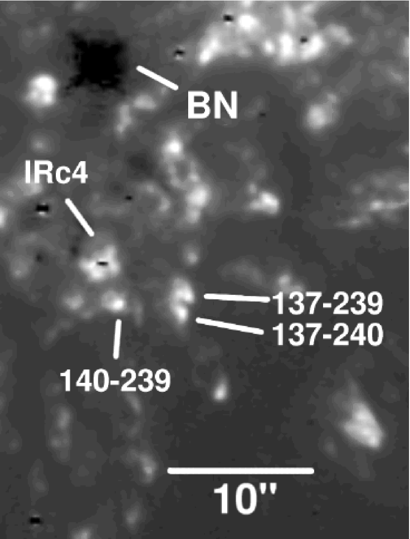
Figure 7: H₂ 1–0 S(1) image of 137–239, 137–240, and 140–239. The maximum brightness in these features is 1.1$\times 10^{-2}$ ergs s^-1cm^-2sr^-1. North is up and east is to the left.

4.1.3 142–240, 143–239, and 144–237

These three objects are shown in H₂ 1–0 S(1) emission in Figure 8. 142–240 is a blunt, bow-shaped object southeast of the star at the head of IRc4. It is bright in H₂ and Fe II, and much fainter in S II and O I (Schultz et al., 2007). The Fe II emission (Schultz et al., 2007) is more extended than the H₂, suggesting these transitions sample different regions. For 142–240, we deduce a C shock velocity of 42 km s^-1 and a pre-shock density of $10^{4.3}$ cm^-3. 142–240 is accompanied on its eastern side by a fainter, larger bow-shaped region of Fe II emission - 143–239 - which is not seen in S II and O I (Schultz et al., 2007). From its H₂ emission, which is blue-shifted (Schultz & Burton, 2007), 143–239 appears to arise from a J-shock: from Figure 4, the velocity and density would be in excess of 100 km s^-1 and $10^{7}$ cm^-3 respectively. A density this high might be expected to produce water masers, and indeed Gaume et al. (1998) find a water maser within the error box of 143–239. 143–239 connects to 144–237 - a bright knot of Fe II (Schultz et al., 2007) and H₂ emission 4.″4 to the northeast of 142–240. Similar to 143–239, 144–237 exhibits blue-shifted emission (Schultz & Burton, 2007), with a deduced shock velocity of 38 km s^-1 and a pre-shock density of $10^{4.3}$ cm^-3. There is also faint Fe II emission slightly ($\sim 0.^{\prime\prime}6$) north of the H₂ emission (Schultz et al., 2007). If this Fe II is associated with 144–237, it may be that 144–237 is moving in the direction of BN or that the bow shock is asymmetric.

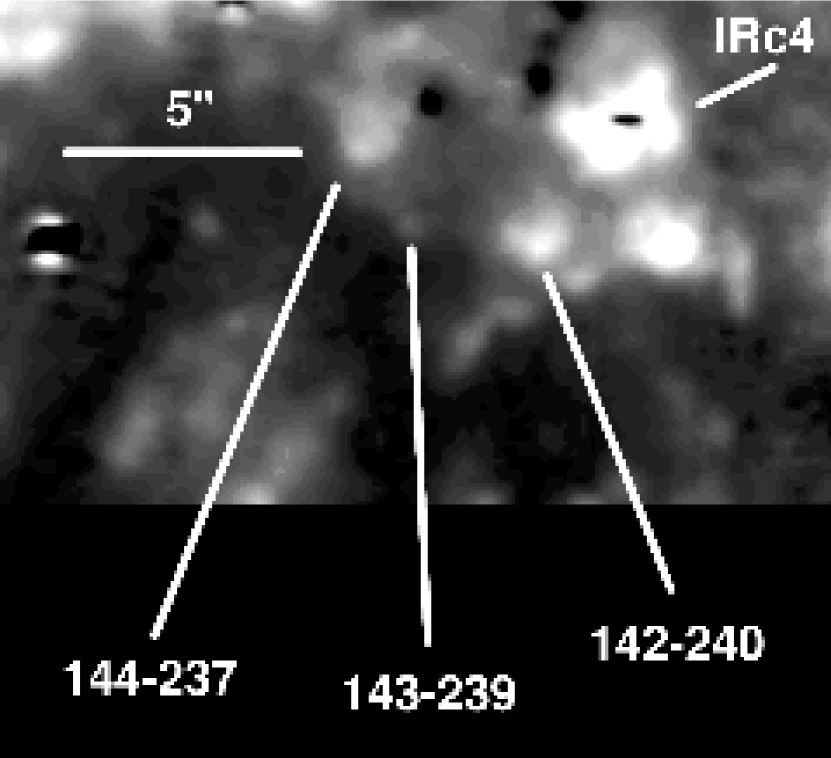
Figure 8: H₂ 1–0 S(1) image of 142–240, 143–239, and 144–237. The maximum brightness in these features is 5.5$\times 10^{-3}$ ergs s^-1cm^-2sr^-1. North is up and east is to the left.

4.1.4 152–229 and 143-225

Chrysostomou et al. (1997) identified 152–229 as a bow shock - their bullet #6. Our H₂, Fe II, and 2.15 µm continuum emission is shown in Figure 9. O’Dell et al. (1997a) found that S II emission in this region is blue-shifted. Gustafsson et al. (2003) found a peak velocity of -21 km s^-1 and a displacement of 0.″2 between the emission peak and the location of the maximum velocity. From the direction of this displacement, they deduced that the shock is propagating towards BN (roughly between 2 and 3 o’clock in Figure 9). In disagreement with Gustafsson et al. (2003), Doi et al. (2002) found from the proper motion of the S II emission, that 152–229 is moving slightly north of east - away from BN/IRc2 - with a transverse velocity of 50 km s^-1. Chrysostomou et al. (1997) found 152–229 to have a FWZI of 110 km s^-1. The estimated shock velocity and pre-shock density are 27 km s^-1 and $10^{5.0}$ cm^-3. Paper (1) noted that the H₂ knot has a pointed cap of Fe II emission on the southeast side of the object (the blue arc in Figure 9), away from the putative exciting source (BN/IRc2) of the outflow. The positioning and morphology strongly suggests a bow shock in which strong shocks producing the Fe II emission form on the leading surface of the bow while weaker shocks producing H₂ emission form behind it. The cap is also seen in the S II and O I images of O’Dell et al. (1997a) and is possibly also visible in high-velocity S II emission (O’Dell et al., 1997b); this may be the unlabelled S II knot northeast of 147–234.

Chrysostomou et al. (1997) also identified 143–225 as a bow shock - their bullet #8, with a a FWZI of 140 km s^-1. 143–225 is among the most blue-shifted features in the outflow (Schultz & Burton, 2007) and may be a bow shock approaching us at a low angle. The H₂ emission is shown in Figure 10. The deduced shock velocity and pre-shock density are 27 km s^-1 and $10^{5.8}$ cm^-3. The shape suggests that it is a bow shock pointed slightly north-northwest, which would mean the origin of the feature would be somewhere to the south-southeast - roughly opposite to the direction of BN.

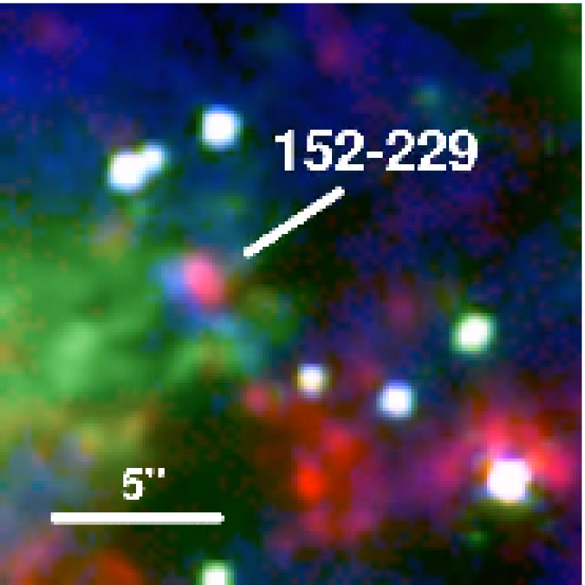
Figure 9: False color image of 152–229. Red is H₂ 1–0 S(1), green is the 2.15 µm continum, and blue is Fe II. North is up and east is to the left.

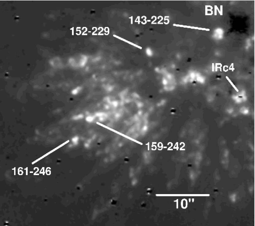
Figure 10: H₂ 1–0 S(1) image of 143–225, 152–229, 159–242 and 161–246. The maximum brightness in these features is 1.8$\times 10^{-2}$ ergs s^-1cm^-2sr^-1. North is up and east is to the left.

4.2 Knots

4.2.1 HH 208

HH 208, approximately $7^{\prime\prime}$ west of BN, was first discovered by Axon & Taylor (1984). The S II and O I HST images of O’Dell et al. (1997b) clearly show a number of small features. Based on S II and O III images, O’Dell et al. (1997a) identified three knots in HH 208. The detection of optical features suggests that the extinction to HH 208 is lower than to other H₂ features, implying it lies more in the foreground. Figure 11 shows our H₂, Fe II, and continuum images, along with our knot identifications. The HH 208 H₂ emission takes the form of discrete clumps, whereas the adjacent H₂ emission has a more fingerlike appearance. It is difficult to discern what process has created this collection of features.

Knot A is the faintest of the 2.12 µm H₂ knots, but is the original HH 208 - seen in both S II and O I. O’Dell et al. (1997b) showed images of knot A in several filters, and noted that a line drawn through HH 208 and HH 208NW terminates near the proplyd 154–240. They suggested that 154–240 may be the source of HH 208, but the line drawn (which is symmetric through HH 208NW but not through the rest of the object) also falls near IRc2 and radio sources “I” and “n”. Doi et al. (2002) found no net proper motion of knot A. The structure of the bright core of knot A did change in a disorganized fashion between 1995 and 2000, which corresponds to motions over a range of about 50 km s^-1. Based on the high-velocity, blue-shifted emission lines, they further suggested that HH 208 is moving almost directly at us, rather than being connected to 154–240. In our data, knot A is the most extreme position - being beyond our grid of C-shock models. It is certainly higher velocity than any other HH 208 location, but may either be a high density ($>10^{7}$ cm^-3) J-shock, or a low density ($<10^{4}$ cm^-3) C-shock. The position of knot B, serving as a bridge between knot A and the rest of the object, is suggestive of a relationship between the forbidden-line and H₂ emission. At 42 km s^-1 and $10^{4.5}$ cm^-3, knot B has the second lowest density after knot U.

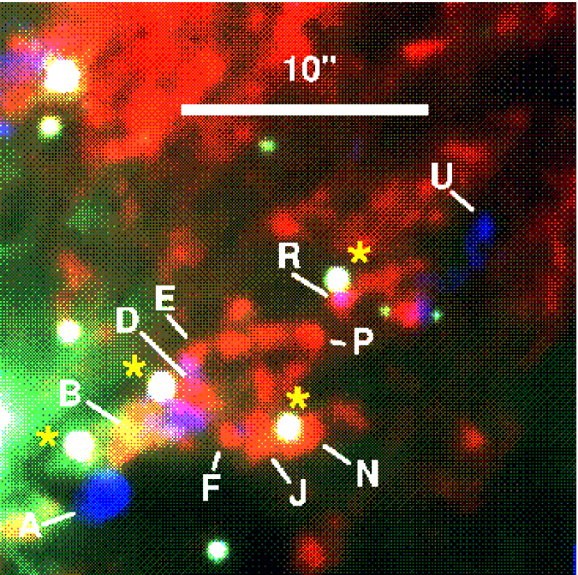
Figure 11: False color image of HH 208 with features discussed in this paper labelled. Red is H₂ 1–0 S(1), green is the 2.15 µm continum, and blue is Fe II 1.64 µm. The gold star symbols denote stars. North is up and east is to the left.

The arrangement of knots D-E-P-N-J-F is suggestive of the “ring” that Schild et al. (1997) pointed out in the northeastern edge of the Orion H₂ emission. The HH208 knots have deduced shock parameters in the 27–40 km s^-1 and $10^{4.5}$ – $10^{5.2}$ cm^-3 ranges, with no clear pattern. However, there may be some excitation gradient with distance from B. Around knots B-D-E, the purple features show where the H₂ and the Fe II emission coincide and the purple disappears beyond E. Since forbidden line emission arises from fast J-shocks, in these regions at least, the spatial coincidence of H₂ and Fe II emission may be inconsistent with our general result that the H₂ emission in HH 208 arises in C-shocks. The knot of high-velocity S II emission designated HH 208NNW by O’Dell et al. (1997a) corresponds to the Fe II emission we find accompanying H₂ knots D-E-F; this emission can also be seen in combined S II and O I emission in Figure 2 of O’Dell et al. (1997b). Farther away, knots J and N together form Object #11 of Chrysostomou et al. (1997), one of the regions from which they detected discrete high velocity H₂ emission. Knot P shows neither forbidden line emission nor high-velocity H₂ emission.

Knots R and U together form HH 208NW (O’Dell et al., 1997a). Knot R shows optical forbidden line emission, including high-velocity, blue-shifted S II emission (O’Dell et al., 1997a). The motion of R (129–216) in the plane of the sky is 49 km s^-1, and of U (126–214) is 65 km s^-1 (Doi et al., 2002), both roughly to the west on a path that would have recently traversed the B-D-E-N-J-F ring. These proper motions put both these objects in the vicinity of BN/I/n around 1000 years ago (Doi et al., 2002), consistent with many other H₂ features in the BN region, but significantly earlier than the 500 year old BN/I/n break-up (Rodríguez et al., 2005; Gómez et al., 2005). In our data, knot R shows the highest pre-shock density ($10^{5.5}$ cm^-3) but the lowest shock velocity (26 km s^-1) in HH 208 - suggesting the H₂ is not in the same region which produces the high velocity S II emission. Knot U ties with B for the second highest velocity (42 km s^-1) and has the lowest density ($10^{4.0}$ cm^-3). Although they may be unrelated to the B-D-E-N-J-F ring, knot U (or perhaps knot R) may be faster-moving material - a wind or knot - that impacted the ambient material to create the ring. Knot A could be a faster moving section of the expanding ring which is moving towards us. The ambient material would then have been a local H₂ clump or even the core of a single, low mass star forming region.

4.2.2 159–242 and 161–246

159–242 and 161–246 - in the southwestern lobe of the outflow - are part of OMC Pk2 (Beckwith et al., 1978). Gustafsson et al. (2003) found 159–242 (their object 6) to have a peak velocity of +11 km s^-1 and 161–246 (the western half of this knot is their object 19) to have a peak velocity of -15 km s^-1. Applying shock models to their 2.12 µm 1–0 S(1) flux measurements, Vannier et al. (2001) derived a pre-shock density of $\sim 10^{6}$ cm^-3, yielding a mass in 161–246 of 0.1 to 0.15 M_⊙, making it the most massive clump in their field. This led them to suggest that the clump is a candidate site for low-mass star formation. Kristensen et al. (2003) expanded upon that work by including 2-1 S(1) images; revising their shock models in light of the new data led them to conclude that the density is an order of magnitude greater than Vannier et al. (2001) calculated. Kristensen et al. (2003) also concluded that the 2-1 S(1)/1-0 S(1) flux ratio included a contribution due to radiative excitation from $\theta^{1}$C Ori, as well as to shocks. They were unable to reproduce both brightness and line ratios with a single type of shock, and therefore suggested that the shock contribution to the emission is composed of C-shocks in the interior of the clump, with J-shocks on the exterior. Our H₂ emission is shown in Figure 10. From our analysis, 159–242 and 161–246 are well fit by shock velocities of 41 and 42 km s^-1 and much lower pre-shock densities of $10^{4.5}$ and $10^{4.4}$ cm^-3. This suggests that the material producing the 2.12 µm 1–0 S(1) emission is insufficient to support even low mass star formation. We do find that the line ratio is about 50% higher in a small region 0.9″ east of the maximum H₂ emission in 159–242, implying a higher shock velocity and lower density there, consistent with the exterior J-shock proposed by Kristensen et al. (2003).

5 Summary

From 0.″2 (90 AU) angular resolution HST NICMOS narrowband images of OMC-1, which resolve individual shocks, we estimate the brightnesses of H₂ transitions at 1.89 and 2.12 µm for 23 features. A comparison of the data with shock models shows that most of the data cannot be fitted by J-shocks, but are well matched by C-shocks with shock velocities in the range of 20–45 km s^-1 and preshock densities of $10^{4}-10^{6}$ cm^-3. The narrow range of shock velocities is not surprising since both slower C-shocks and faster J-shocks produce weaker H₂ emission and would not have been detected. Although there are many shock features in the OMC-1 region, most of the features appear to be well-characterized by a limited range of shock velocities and preshock densities, supporting the possibility of a common origin. Additionally, these values confirm the findings of larger beam studies, which averaged over a number of individual shocks. Two objects - 143–239 and HH208A - are possibly due to J-shocks and the former does coincide with a known water maser. Optical forbidden line measurements of some features in HH 208 require fast J-shocks for excitation; we cannot explain this apparent discrepancy.

References

- Allen & Burton (1993) Allen, D.A. and Burton, M.G. 1993 Nature, 363, 54 (AB)
- Axon & Taylor (1984) Axon, D.J. and Taylor, K. 1984 MNRAS 207 241
- Beckwith et al. (1978) Beckwith, S., Persson, S.E., Neugebauer, G., and Becklin, E.E. 1978 ApJ 223 464
- Beckwith et al. (1983) Beckwith, S., Evans II, N.J., Gatley, I., Gull, G., and Russell, R.W. 1983 ApJ 264 152
- Cardelli et al. (1989) Cardelli, J.A., Clayton, G.C., and Mathis, J.S. 1989 ApJ 345 245
- Chernoff et al. (1982) Chernoff, D.F., McKee, C.F., and Hollenbach, D.J. 1982 ApJ 259 L7