Flux, Gaugino Condensation and Anti-Branes in Heterotic M-theory

James Gray¹, André Lukas² and Burt Ovrut³

¹Institut d’Astrophysique de Paris and APC, Université de Paris 7,

98 bis, Bd. Arago 75014, Paris, France

²Rudolf Peierls Centre for Theoretical Physics, University of Oxford,

1 Keble Road, Oxford OX1 3NP, UK

³Department of Physics, University of Pennsylvania,

Philadelphia, PA 19104–6395, USA

We present the potential energy due to flux and gaugino condensation in heterotic M-theory compactifications with anti-branes in the vacuum. For reasons which we explain in detail, the contributions to the potential due to flux are not modified from those in supersymmetric contexts. The discussion of gaugino condensation is, however, changed by the presence of anti-branes. We show how a careful microscopic analysis of the system allows us to use standard results in supersymmetric gauge theory in describing such effects - despite the explicit supersymmetry breaking which is present. Not surprisingly, the significant effect of anti-branes on the threshold corrections to the gauge kinetic functions greatly alters the potential energy terms arising from gaugino condensation.

                                           

¹email: gray@iap.fr
²email: lukas@physics.ox.ac.uk
³email: ovrut@elcapitan.hep.upenn.edu

1 Introduction

In [1], the perturbative four-dimensional effective action of heterotic M-theory compactified on vacua containing both branes and anti-branes in the bulk space was derived. That paper concentrated specifically on those aspects of the perturbative low energy theory which are induced by the inclusion of anti-branes. Hence, for clarity of presentation, the effect of background $G$-flux on the effective theory was not discussed. Furthermore, non-perturbative physics, namely gaugino condensation and membrane instantons, was not included. However, all three of these contributions are required for a complete discussion of moduli stabilization, ${\cal{N}}=1$ supersymmetry breaking and the cosmological constant. Therefore, in this paper, we extend the results of [1] to include the effects of flux and gaugino condensation. Another piece of the effective theory, that is, the contribution of membrane instantons, will be presented elsewhere [2]. There is of course a vast literature on the subject of moduli stabilization, flux and gaugino condensation in heterotic theories. Some recent discussions of various aspects of these topics appear in [3, 4, 5, 6, 7, 8, 9, 10, 11, 12].

A strong motivation for attempting to find stable vacua in Calabi-Yau compactifications of heterotic theories comes from the advantages that such constructions enjoy in particle physics model building. For example, models with an underlying ${\rm SO}(10)$ GUT symmetry can be constructed where one right handed neutrino per family occurs naturally in the $\bf 16\rm$ multiplet and gauge unification is generic due to the universal gauge kinetic functions in heterotic theories. Recent progress in the understanding of non-standard embedding models [13, 14, 15, 16] and the associated mathematics of vector bundles on Calabi-Yau spaces [17, 18, 19, 20] has led to the construction of effective theories close to the Minimal Supersymmetric Standard Model (MSSM), see [21, 22, 23, 24, 25, 26]. This has opened up new avenues for heterotic phenomenology. For example, one can proceed to look at more detailed properties of these models such as $\mu$ terms [27], Yukawa couplings [28], the number of moduli [29] and so forth. Other groups are also making strides in heterotic model building, see for example [30, 31, 32, 33, 34, 35].

The addition of $G$-flux to the formalism described in [1] is, as we will show in this paper, relatively straightforward. In contrast, it is not at first obvious how to incorporate gaugino condensation into this explicitly non-supersymmetric compactification of M-theory. The reason is that almost everything we know about this non-perturbative phenomenon is based on the dynamics of unbroken ${\cal N}=1$ supersymmetric gauge theories. However, by carefully analyzing the limit where the usual discussions of gaugino condensation are applied, we will show that our non-supersymmetric system reverts to a globally supersymmetric gauge theory. This fact allows us to construct the condensation induced potential energy terms in the presence of anti-branes using a component action approach similar to that of [36].

The plan of this paper is as follows. In the next section, we briefly review those aspects of [1] which are required for the current work. In Section 3, we review the subject of flux in supersymmetric heterotic M-theory. In Section 4, the effects of $G$-flux in heterotic M-theory vacua which include anti-branes are explicitly computed. Gaugino condensation in the presence of anti-branes is then introduced in Section 5. We begin by describing how the potential energy terms induced by this effect can be calculated in terms of the condensate itself. It is then shown how one can explicitly evaluate the condensate as a function of the moduli fields. Finally, we conclude in Section 6 by writing out, in full, the effective potential energy we have obtained by compactifying heterotic M-theory in the presence of anti-branes, $G$-flux and gaugino condensation.

2 Anti-Branes in Heterotic M-Theory

The low energy effective Lagrangian of heterotic M-theory compactified on vacua containing bulk space branes and anti-branes, but ignoring $G$-flux and non-perturbative effects, was constructed in [1]. In this section, we provide a brief summary of the aspects of [1] which are important in the current paper. The basic vacuum configuration which we consider, as viewed from five dimensions, is depicted in Figure 1.

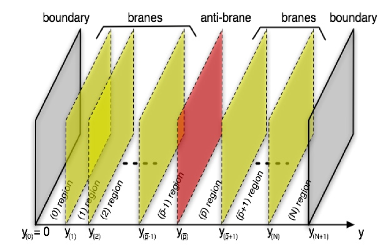
Figure 1: The brane configuration in five-dimensional heterotic M-theory

We include an arbitrary number of three-branes in the vacuum, but, for clarity of notation, restrict the discussion to a single anti three-brane. Our results extend almost trivially to the case where multiple anti-branes are present. The (anti) three-branes arise as the low energy limit of (anti) M5-branes wrapped on holomorphic curves in the internal Calabi-Yau threefold. We will often refer to the (anti) three-branes simply as (anti-) branes. A more detailed discussion of this setup is provided in [1]. As shown in Figure 1, we label the extended objects with a bracketed index $(p)$ ranging from $(0)$ to $(N+1)$. The values $(0)$ and $(N+1)$ correspond to the orbifold fixed planes, $(\bar{p})$ labels the anti-brane and the remaining $(p)$ values are associated with the branes. The bulk regions are labeled by the same index as the brane which borders them on the left. Fields associated with the world volume of a given extended object or with a certain region of the bulk are often labelled with the associated index.

In [1], our starting point was the five-dimensional action describing the compactification of Hořava-Witten theory on a Calabi-Yau threefold $X$ in the presence of both M5 branes and an anti-M5 brane. The bosonic field content of this theory is as follows. Let $\alpha,\beta,\ldots=0,\dots,4$ be the five-dimensional bulk space indices, $\mu,\nu,\ldots=0,\dots,3$ label the four-dimensional Minkowski space indices and $y$ be the coordinate of the $S^{1}/{\mathbb{Z}_{2}}$ orbifold interval. Additionally, we let $i,j,k,\ldots=1,\dots,h^{1,1}$, $\underline{a},\underline{b},\ldots=1,\dots,h^{2,1}$ and $\underline{A},\underline{B},\ldots=1,\dots,h^{2,1}+1$, where $h^{1,1}$ and $h^{2,1}$ are the dimensions of the $H^{1,1}(X)$ and $H^{2,1}(X)$ cohomology groups respectively. Then, in the bulk space we have the graviton, $g_{\alpha\beta}$, $h^{1,1}$ Abelian vector fields ${{\cal A}_{\alpha}}^{k}$ with field strengths ${{\cal F}_{\alpha\beta}}^{k}$, a real scalar field $V$, $h^{1,1}$ real scalar fields $b^{k}$ which obey the condition $d_{ijk}b^{i}b^{j}b^{k}=6$ (the $d_{ijk}$ being the intersection numbers on the Calabi-Yau threefold) and, therefore, constitute $h^{1,1}-1$ degrees of freedom, $h^{2,1}$ complex scalar fields ${\mathfrak{z}}^{\underline{a}}$, $2(h^{2,1}+1)$ real scalar fields ${\xi}^{\underline{A}}$, $\tilde{\xi}_{\underline{B}}$ with their field strengths ${{\cal{X}}^{\underline{A}}}_{\alpha}$, ${{\cal{X}}_{\underline{B}}}_{\beta}$ and the three-form $C_{\alpha\beta\gamma}$ with its field strength $G_{\alpha\beta\gamma\delta}$. Of these bulk fields, $V$, ${\mathfrak{z}}^{\underline{a}}$, $g_{\mu\nu}$, $g_{yy}$, $b^{k}$, $C_{\mu\nu y}$ and ${\cal A}^{k}_{y}$ are even under the ${\mathbb{Z}}_{2}$ orbifold projection, while $g_{\mu y}$, $\xi^{\underline{A}}$, $\tilde{\xi}_{\underline{B}}$, ${\cal A}^{k}_{\mu}$, $C_{\mu\nu\gamma}$ are odd.

In addition, there are extra degrees of freedom living on the extended sources in the vacuum. On each of the two four-dimensional fixed planes, one finds ${\cal N}=1$ gauge supermultiplets. These contain gauge fields $A_{(p)\mu}$ indexed over the adjoint representation of the unbroken gauge group ${\cal{H}}_{(p)}\subseteq E_{8}$ for $p=0,N+1$. The associated fields strengths are denote by $F_{(p)\mu\nu}$. Furthermore, on the fixed planes there are ${\cal N}=1$ chiral matter supermultiplets with scalar components $C_{(p)}^{Rx}$, $p=0,N+1$ transforming in various representations $R$, with components $x$, of this gauge group. Details of the origin and structure of the matter sector can be found in the Appendix of [1]. The world volume fields associated with the three-branes are as follows. First, each brane $(p)$ has an embedding coordinate, that is, the brane position, $y_{(p)}$ and a world volume scalar $s_{(p)}$. Second, each brane supports an ${\cal N}=1$ gauge supermultiplet with structure group $U(1)^{g_{(p)}}$ where $g_{(p)}$ is the genus of the curve wrapped by brane $(p)$. These contain the Abelian gauge fields $A_{(p)\mu}^{u}$, where $u=1,\dots,g_{(p)}$. The associated field strengths are denoted by $E^{u}_{(p)}$. In general, there will be additional chiral multiplets describing the moduli space of the curves around which the M5 and anti-M5 branes are wrapped. Furthermore, there may be non-Abelian generalizations of the gauge field degrees of freedom when branes are stacked. However, these multiplets are not vital to our discussion and, therefore, we shall not explicitly take them into account.

Given this field content, the five-dimensional action describing Hořava-Witten theory compactified on an arbitrary Calabi-Yau threefold in the presence of M5 branes and an anti-M5 brane is given by

$$S=-\frac{1}{2\kappa_{5}^{2}}\int d^{5}x\sqrt{-g}\left[\frac{1}{2}R+\frac{1}{4}G_{kl}(b)\partial b^{k}\partial b^{l}+\frac{1}{2}G_{kl}(b){\cal F}^{k}_{\alpha\beta}{\cal F}^{l\alpha\beta}+\frac{1}{4}V^{-2}(\partial V)^{2}+\lambda(d_{ijk}b^{i}b^{j}b^{k}-6)\right.$$

$$\left.+\frac{1}{4}{\cal K}_{\underline{a}\underline{\bar{b}}}({\mathfrak{z}})\partial{\mathfrak{z}}^{\underline{a}}\partial\bar{{\mathfrak{z}}}^{\underline{\bar{b}}}-V^{-1}(\tilde{\cal X}_{\underline{A}\alpha}-\bar{M}_{\underline{A}\underline{B}}({\mathfrak{z}}){\cal X}_{\alpha}^{\underline{B}})([\textnormal{Im}{(M({\mathfrak{z}}))}]^{-1})^{\underline{A}\underline{C}}(\tilde{\cal X}_{\underline{C}}^{\alpha}-M_{\underline{C}\underline{D}}({\mathfrak{z}}){\cal X}^{\underline{D}\alpha})\right.$$

$$\left.+\frac{1}{4!}V^{2}G_{\alpha\beta\gamma\delta}G^{\alpha\beta\gamma\delta}+m^{2}V^{-2}G^{kl}(b)\hat{\beta}_{k}\hat{\beta}_{l}\right]$$

$$-\frac{1}{2\kappa_{5}^{2}}\int\left(\frac{2}{3}d_{klm}{\cal A}^{k}\wedge{\cal F}^{l}\wedge{\cal F}^{m}+2G\wedge((\xi^{\underline{A}}\tilde{\cal X}_{\underline{A}}-\tilde{\xi}_{\underline{A}}{\cal X}^{\underline{A}})-2m\hat{\beta}_{k}{\cal A}^{k})\right)$$

$$-\int d^{5}x\;\delta(y)\sqrt{-h_{(0)}}\,\left[\frac{m}{\kappa_{5}^{2}}V^{-1}b^{k}\tau^{(0)}_{k}+\frac{1}{8\pi\alpha_{\textnormal{GUT}}}V\rm{tr}(F_{(0)}^{2})+{\cal G}_{(0)RS}D_{\mu}C^{Rx}_{(0)}D^{\mu}\bar{C}^{S}_{(0)x}\right.$$ (1)

$$\left.+V^{-1}{\cal G}^{RS}_{(0)}\frac{\partial W_{(0)}}{\partial C^{Rx}_{(0)}}\frac{\partial\bar{W}_{(0)}}{\partial\bar{C}^{S}_{(0)x}}+{\rm tr}(D_{(0)}^{2})\right]$$

$$-\int d^{5}x\;\delta(y-\pi\rho)\sqrt{-h_{(N+1)}}\,\left[\frac{m}{\kappa_{5}^{2}}V^{-1}b^{k}\tau^{(N+1)}_{k}+\frac{1}{8\pi\alpha_{\textnormal{GUT}}}V{\rm tr}(F_{(N+1)}^{2})+{\cal G}_{(0)RS}D_{\mu}C^{Rx}_{(N+1)}D^{\mu}\bar{C}^{S}_{(N+1)x}\right.$$

$$\left.+V^{-1}{\cal G}^{RS}_{(0)}\frac{\partial W_{(N+1)}}{\partial C^{Rx}_{(N+1)}}\frac{\partial\bar{W}_{(N+1)}}{\partial\bar{C}^{S}_{(N+1)x}}+{\rm tr}(D_{(N+1)}^{2})\right]$$

$$-\frac{1}{2\kappa_{5}^{2}}\int d^{5}x\;\sum_{p=1}^{N}(\delta(y-y_{(p)})+\delta(y+y_{(p)}))\left\{\sqrt{-h_{(p)}}\,\left[mV^{-1}\tau^{(p)}_{k}b^{k}+\frac{2(n_{(p)}^{k}\tau^{(p)}_{k})^{2}}{V(\tau^{(p)}_{l}b^{l})}j_{{(p)}\mu}j^{\mu}_{(p)}\right.\right.$$

$$\left.\left.+[\textnormal{Im}{\Pi}]_{{(p)}uw}E^{u}_{{(p)}\mu\nu}E^{w\mu\nu}_{(p)}\right]-4\hat{C}_{(p)}\wedge\tau^{(p)}_{k}d(n^{k}_{(p)}s_{(p)})-2[\textnormal{Re}{\Pi}]_{(p)uw}E^{u}_{(p)}\wedge E^{w}_{(p)}\right\}.$$

Here $\kappa_{5}$ and $\alpha_{GUT}$ are given by

$$\kappa_{5}^{2}=\frac{\kappa_{11}^{2}}{v},\quad\alpha_{GUT}=\frac{(4\pi\kappa_{11}^{2})^{2/3}}{v},$$ (2)

where $\kappa_{5}$ and $\kappa_{11}$ are $5$- and $11$-dimensional Planck constants respectively, $v$ is the reference Calabi-Yau volume and constant $m$ is the reference mass scale

$$m=\frac{2\pi}{v^{\frac{2}{3}}}\left(\frac{\kappa_{11}}{4\pi}\right)^{\frac{2}{3}}.$$ (3)

The above expressions describe, in the order presented, the bulk space, the fixed planes and the world volumes of the M5 and anti-M5 branes. The metrics $G_{kl}(b)$, ${\cal{K}}_{\underline{a}\underline{\bar{b}}}({\mathfrak{z}})$ as well as the matrix $M_{\underline{A}\underline{B}}({\mathfrak{z}})$ appearing in the bulk space term are defined in Appendix A of [1]. Their precise form is not required in this paper. The $d_{klm}$ coefficients are the intersection numbers of the Calabi-Yau threefold. The integers $\tau_{k}^{(p)}$ are the tensions of the branes, anti-branes and fixed planes. Charges on individual branes are simply labeled by $\beta^{(p)}_{k}$ and are equal to the associated tensions in the case of branes and fixed planes and equal in magnitude, but opposite in sign, in the case of the anti-brane. The anti-brane is taken to be associated with a purely anti-effective curve for simplicity. The $\hat{\beta}_{k}$ coefficients are the sum of the charges on all extended sources to the left of where the bulk theory is being considered. We will frequently denote quantities associated with the anti-brane by a bar. Hence, the tension of the anti-brane is denoted by $\bar{\tau}_{k}=\tau^{(\bar{p})}_{k}$. The metrics ${\cal{G}}_{(p)RS}$, the matter field superpotentials $W_{(p)}$ and the D-terms $D_{(p)}$ with $p=0,N+1$ appearing in the boundary plane terms are defined in Appendix B of [1]. Again, their precise form is not required for the analysis in this paper. The quantities

$$n_{(p)}^{k}=\frac{\beta_{k}^{(p)}}{\Sigma_{l=1}^{h^{1,1}}\beta_{l}^{(p)2}}$$ (4)

are the normalized version of the three-brane charges and we have used the definition

$$j_{(p)\mu} = \frac{\beta^{(p)}_{k}}{n_{(p)}^{l}\beta^{(p)}_{l}}(d(n^{k}_{(p)}s_{(p)})-\hat{{\cal A}}^{k}_{(p)})_{\mu}.$$ (5)

Hats on field quantities denote pullbacks of the corresponding bulk variable onto the extended object under consideration. The matrix $\Pi_{(p)uw}$ appearing in the world volume brane terms is the period matrix of the curve on which the $p$-th brane or anti-brane is wrapped. This is defined in Appendix C of [1]. Finally, the quantities $h_{(p)}$ are the induced metrics on the boundary planes, branes and the anti-brane. It is important to note that despite the appearance of an anti M5-brane in the vacuum, action (2) is ${\cal{N}}=1$ supersymmetric, both in the five-dimensional bulk space and on all four-dimensional fixed planes and branes. The reason for this is that the dimensional reduction was carried out with respect to the supersymmetry preserving Calabi-Yau threefold, and did not explicitly involve the anti M5-brane. However, as we now briefly discuss, the anti M5-brane does enter the dimensional reduction of the theory to four-dimensions, explicitly breaking its ${\cal{N}}=1$ supersymmetry.

In [1], we described how the presence of an anti-brane in the bulk space of a heterotic M-theory vacuum changes the warping in the extra dimensions. We showed that this back-reaction is manifested by a quadratic contribution to the warping. It is interesting to note that this contribution derives simply from the failure of the tensions of the extended objects to sum to zero in the case where anti-branes are present. This property of the source terms is responsible for all of the major changes to the perturbative theory. The only bulk fields involved in the generalized domain wall solution including an anti-brane are the metric $g_{\alpha\beta}$, the volume modulus $V$ and the Kähler moduli $b^{k}$. We take as our metric ansatz

$$ds^{2}_{5}=a(x^{\mu},y)^{2}g_{4\mu\nu}(x^{\mu})dx^{\mu}dx^{\nu}+b(x^{\mu},y)^{2}dy^{2}.$$ (6)

It turns out to be helpful to introduce a function which encodes the standard linear warping functions of heterotic M-theory in a usefully normalized manner. It is given by

$$h_{(p)k}(z)=\sum^{p}_{q=0}\tau^{(q)}_{k}(z-z_{(q)})-\frac{1}{2}\sum_{q=0}^{N+1}\tau^{(q)}_{k}z_{(q)}(z_{(q)}-2)-\delta_{k}\;.$$ (7)

The $z$ which appears here is defined by $z=y/\pi\rho$, where $\pi\rho$ is the reference length of the orbifold interval and $y$ is the coordinate of the fifth dimension. Each $z_{(q)}$ is the $\pi\rho$ normalized position modulus for the $q$-th brane or anti-brane. Note that the fixed planes are located at $z_{(0)}=0$ and $z_{(N+1)}=1$ respectively. In expression (7),

$$\delta_{k}=\frac{1}{2}(\bar{\tau}_{k}-\bar{\beta}_{k})=\bar{\tau}_{k}.$$ (8)

The quantity $h_{(p)k}$ has been defined so that its orbifold average is zero. This property enables us to extract definitions of the zero modes of the compactification which lead to a four-dimensional action in a sensible form, without the need to use field redefinitions.

Using these definitions and the equations of motion for $V$ and $b^{k}$, we find the following non-supersymmetric domain wall ansatz around which the theory will be reduced to four-dimensions. It is given by

$$\frac{a_{(p)}}{a_{0}} = 1-\epsilon_{0}\frac{b_{0}}{3V_{0}}b_{0}^{k}\left[h_{(p)k}+\delta_{k}\left(z^{2}-\frac{1}{3}\right)\right]$$ (9)

$$\frac{V_{(p)}}{V_{0}} = 1-2\epsilon_{0}\frac{b_{0}}{V_{0}}b_{0}^{k}\left[h_{(p)k}-\delta_{k}\left(z^{2}-\frac{1}{3}\right)\right]$$ (10)

$$b_{(p)}^{k} = b_{0}^{k}+2\epsilon_{0}\frac{b_{0}}{V_{0}}\left[\left(h_{(p)}^{k}-\frac{1}{3}h_{(p)l}b_{0}^{k}b_{0}^{l}\right)-\left(\delta^{k}-\frac{1}{3}\delta_{l}b_{0}^{k}b_{0}^{l}\right)\left(z^{2}-\frac{1}{3}\right)\right],$$ (11)

where

$$\epsilon_{0}=\pi\rho m$$ (12)

with $m$ defined in (3). The remaining notation is as explained earlier, with the one addition that the “$0$” subscript on $a_{0}$, $b_{0}$, $V_{0}$ and $b^{k}_{0}$ denotes quantities which are functions of the four uncompactified coordinates only. It is these functions that become the moduli when we dimensionally reduce on this ansatz to obtain the effective four-dimensional action. Note that we have not given an expression for the warping of the metric coefficient $b$. This is because this $y$ dependence can be removed by a coordinate redefinition and, hence, does not enter the calculation of the four-dimensional effective action.

We emphasize several points about this result which will be important in this paper. First, the $z$ independent factors have been defined such that $a_{0}$, $b_{0}$, $V_{0}$ and $b^{k}_{0}$ are simply the orbifold averages of $a$, $b$, $V$ and $b^{k}$ respectively. This proves to be useful in performing the dimensional reduction around this configuration. Second, upon taking $\delta_{k}\rightarrow 0$ one recovers the conventional results for heterotic M-theory, given, for example, in [37]. In particular, the quadratic pieces of the warping correctly disappear as we turn the anti-brane into an M5 brane in this manner. Note that in each of the above expressions the warping occurs with the same multiplicative factor, specifically $\epsilon_{0}\frac{b_{0}}{V_{0}}$. In [1, 38], it was shown that the four-dimensional effective theory is an expansion in the parameters $\epsilon_{S}$ and $\epsilon_{R}$ given by

$$\epsilon_{S}=\pi\left(\frac{\kappa_{11}}{4\pi}\right)^{\frac{2}{3}}\frac{2\pi\rho}{v^{\frac{2}{3}}}\frac{b_{0}}{V_{0}}\;\;\;\;,\;\;\;\;\epsilon_{R}=\frac{v^{\frac{1}{6}}}{\pi\rho}\frac{V_{0}^{\frac{1}{2}}}{b_{0}}.$$ (13)

The first of these is the “strong coupling” parameter which specifies the size of the warping in the orbifold dimension. The second term is the expansion parameter which controls the size of the Calabi-Yau Kaluza-Klein modes. Using (3) and (12), we see that

$$\epsilon_{S}=\epsilon_{0}\frac{b_{0}}{V_{0}},$$ (14)

as it should be.

Further results from [1] will be reproduced as and when required in the following sections.

3 Flux in Supersymmetric Heterotic M-Theory

In this section, we review the subject of flux in supersymmetric Calabi-Yau compactifications of heterotic M-theory. Initially, we will consider heterotic theory from an eleven-dimensional perspective so that a complete understanding is obtained of all of the different fluxes present, including those whose nature is somewhat obscured by the five-dimensional description. Later on in this section, however, having gained this understanding, we revert to the five-dimensional picture which is technically more convenient for the discussion of the addition of anti-branes. The full eleven-dimensional $M$-theory indices will be denoted by $I,J,K,\ldots=0,\dots,9,11$, whereas ten-dimensional indices orthogonal to the orbifold direction $y$ are written as $\bar{I},\bar{J},\bar{K},\ldots=0,\dots,9$. Furthermore, the six-dimensional real coordinates on the Calabi-Yau manifold $(CY_{3})$ will be specified by $A,B,C,\ldots=4,\dots,9$. The associated holomorphic and anti-holomorphic complex coordinates on the threefold are then written as $a,b,c,\ldots=1,2,3$ and $\bar{a},\bar{b},\bar{c},\ldots=1,2,3$ respectively. Finally, the indices $\hat{i},\hat{j},\hat{k},\ldots=4,\dots,9,11$ run over both the $CY_{3}$ and orbifold directions. The material on the non-zero mode of heterotic M-theory reviewed here was first presented in [39, 40, 41, 38].

3.1 The components of $G$ relevant to stable vacua

Let us find the components of the eleven-dimensional background four-form flux $G_{IJKL}$ that can be non-vanishing in a realistic, stable vacuum. To begin, note that there are three possible types of index structure for the four-form $G$.

• One or more 4D indices: The possibilities are $G_{\mu\nu\gamma\delta},G_{\mu\nu\gamma\hat{i}},G_{\mu\nu\hat{i}\hat{j}}$ and $G_{\mu\hat{i}\hat{j}\hat{k}}$.

  • $G_{\mu\nu\gamma\hat{i}},G_{\mu\nu\hat{i}\hat{j}}$ and $G_{\mu\hat{i}\hat{j}\hat{k}}$ all obviously break maximal spacetime symmetry in four dimensions (that is, Poincar$\rm\acute{e}$, de Sitter or anti-de Sitter symmetry) if present in the vacuum. As such, they are not relevant for a discussion of realistic stabilized vacua and will be set to zero.

  • A priori, $G_{\mu\nu\gamma\delta}$ could have an expectation value proportional to the four-dimensional volume element without breaking maximal spacetime symmetry. However, $G$ is intrinsically odd under the Hořava-Witten $\mathbb{Z}_{2}$ and so, since $G_{\mu\nu\gamma\delta}$ has no $y$ index, this component is also odd under the orbifolding. Given this, if non-zero, $G_{\mu\nu\gamma\delta}$ must jump at the orbifold fixed planes. Were there to be such a discontinuity, the exterior derivative $(dG)_{y\mu\nu\gamma\delta}$ would be a delta function at each fixed plane and, hence, require charges of the appropriate index for global consistency. On the fixed planes we have two options, either an $(F\wedge F)_{\mu\nu\gamma\delta}$ or $(R\wedge R)_{\mu\nu\gamma\delta}$ source. However, giving an expectation value to a four-dimensional vector gauge field clearly breaks our requirement of maximal spacetime symmetry. Furthermore, it turns out that $(R\wedge R)_{\mu\nu\gamma\delta}$ for a space of maximal spacetime symmetry vanishes. Therefore, a purely external component of the four-form in a realistic, stable vacuum must also be chosen to be zero. We conclude that, if they are to be non-vanishing, all indices of $G$ must lie on the internal seven-orbifold.

• All indices on the $CY_{3}$: Written in terms of the complex coordinates on the $CY_{3}$, there are three possible index structures for the $G_{ABCD}$ components; $G_{abc\bar{d}},G_{\bar{a}\bar{b}\bar{c}d}$ and $G_{a\bar{b}c\bar{d}}$. Since $G$ is intrinsically odd and $G_{ABCD}$ has no $y$ index, all of these components are odd under the $\mathbb{Z}_{2}$ orbifolding.

• One index on the orbifold and the rest on the $CY_{3}$: In this case there are four possible complex index structures, $G_{abcy},G_{\bar{a}\bar{b}\bar{c}y}$ and $G_{ab\bar{c}y},G_{\bar{a}\bar{b}cy}$, for the $G_{ABCy}$ components. All of these are, however, even under the $\mathbb{Z}_{2}$ due to the $y$ index which they carry.

In summary, if we are interested in stable vacua of heterotic M-theory with maximal spacetime symmetry, we need only consider four-form fluxes with all indices internal to the compactification seven-orbifold. Of these, the $G_{ABCD}$ are odd and the $G_{ABCy}$ even under the $\mathbb{Z}_{2}$ action.

3.2 The Bianchi identity and its sources

The components of $G$ are constrained by the requirement of anomaly freedom to satisfy the Bianchi identity of eleven-dimensional heterotic M-theory with $N$ bulk M5 branes. It follows from the above discussion that the non-vanishing components of $G$ are contained in the seven-dimensional restriction of this identity given by

$$(dG)_{yABCD} = 4\pi\left(\frac{\kappa_{11}}{4\pi}\right)^{\frac{2}{3}}\left[\delta(y)J^{(0)}+\delta(y-\pi\rho)J^{(N+1)}+\frac{1}{2}\sum_{p=1}^{N}J^{(p)}\left(\delta(y-y_{(p)})+\delta(y+y_{(p)})\right)\right]_{ABCD}$$ (15)

The four-form charges localized on the orbifold fixed planes and bulk M5 branes in this expression are

$$J^{(0)} = -\frac{1}{16\pi^{2}}\left(\textrm{tr}F^{(1)}\wedge F^{(1)}-\frac{1}{2}\textrm{tr}R\wedge R\right)|_{y=0}\;,$$ (16)

$$J^{(N+1)} = -\frac{1}{16\pi^{2}}\left(\textrm{tr}F^{(2)}\wedge F^{(2)}-\frac{1}{2}\textrm{tr}R\wedge R\right)|_{y=\pi\rho}\;,$$

$$J^{(p)} = \delta({\cal C}^{(p)}_{2})\;$$

respectively, where $\delta({\cal C}^{(p)}_{2})$ is a delta-function four-form localized on the curve ${\cal C}^{(p)}_{2}$ wrapped by the $p$-th M5 brane. For any two-form $\chi$, we have $\int_{CY_{3}}\chi\wedge\delta({\cal C}^{(p)}_{2})=\int_{{\cal C}^{(p)}_{2}}\chi$. Note that since $d(dG)=0$, it follows that the sources $J^{(p)}$,$p=0,\dots,N+1$ are closed four-forms on the $CY_{3}$.

Integrability conditions arise from the Bianchi identity by integrating both sides of expression (15) over closed 5-cycles. Since the components of the Bianchi identity have a $y$ index, one of the dimensions of the cycle must be the orbifold direction. The remaining dimensions form some closed four-cycle in the Calabi-Yau threefold. The left-hand side of (15), being exact, gives zero upon integration, whereas each term on the right-hand side becomes a topological invariant. We thus obtain the well-known cohomology condition of heterotic M-theory for each choice of four-cycle ${\cal C}_{4}$,

$$-\frac{1}{16\pi^{2}}\int_{{\cal C}_{4}}\textrm{tr}F^{(1)}\wedge F^{(1)}-\frac{1}{16\pi^{2}}\int_{{\cal C}_{4}}\textrm{tr}F^{(2)}\wedge F^{(2)}+\frac{1}{16\pi^{2}}\int_{{\cal C}_{4}}\textrm{tr}R\wedge R+\sum_{p=1}^{N}\int_{{\cal C}_{4}}J^{(p)}=0\;.$$ (17)

The physical interpretation of this condition is simply that the sum of the charges on the compact space must vanish since there is nowhere for the “field lines” to go.

One can expand the charges (16) in terms of the eigenmodes of the Laplacian on the $CY_{3}$ [38]. Consider the two-forms satisfying the eigenmode equation

$$\triangle\omega_{<m>\;AB}=-\lambda_{<m>}^{2}\omega_{<m>\;AB}\;,$$ (18)

where $\triangle$ is the Laplacian and the index $<m>$ labels the eigenmode on the threefold with eigenvalue $-\lambda^{2}_{<m>}$. Note that eigenmodes with different values of $<m>$ may have identical eigenvalues. For example, consider the number of two-form eigenmodes with $\lambda^{2}_{<m>}=0$, that is, the zero modes of $\triangle$. Since by definition these two-forms are harmonic, there are ${\rm dim}H^{2}(X)={\rm dim}H^{(1,1)}$ of them. We will denote these harmonic modes by $\omega_{k}$, where $k=1,\dots,h^{1,1}$. Note that eigenmodes corresponding to a non-vanishing eigenvalue $-\lambda^{2}_{<m>}\neq 0$ are neither harmonic nor, in general, closed forms. The metric on the space of eigenmodes,

$$G_{<m><n>}=\frac{1}{2v}\int_{CY_{3}}{\omega_{<m>}\wedge\ast_{CY_{3}}\omega_{<n>}}$$ (19)

where $\ast_{CY_{3}}$ is the Poincaré duality operator on the $CY_{3}$, is used to raise and lower $<m>$-type indices.

Each of the four-form charges $J^{(p)}$, $p=0,...,N+1$ in (16) can then be expanded as

$$\ast_{CY_{3}}J^{(p)}=\frac{1}{2v^{\frac{2}{3}}}\sum_{<m>}\beta_{<m>}^{(p)}\omega^{<m>}\;.$$ (20)

Using metric (19), it follows that

$$\beta_{<m>}^{(p)}=\frac{1}{v^{1/3}}\int_{CY_{3}}{\omega_{<m>}\wedge J^{(p)}}.$$ (21)

In particular, for the coefficients $\beta_{k}^{(p)}$ corresponding to the zero modes one finds

$$\beta_{k}^{(p)}=\int_{{\cal{C}}_{4k}}{J^{(p)}},$$ (22)

where ${\cal{C}}_{4k}$, $k=1,\dots,h^{1,1}$ are the four-cycles dual to the harmonic $(1,1)$ forms $\omega_{k}$. It then follows from the the cohomology condition (17) that

$$\sum_{p=0}^{N+1}\beta_{k}^{(p)}=0$$ (23)

for each integer $k$. In general, as indicated in (20), the four-form charges in (15) are built out of both harmonic and non-harmonic modes on the $CY_{3}$. There is no similar condition on the sum of the coefficients of the non-harmonic components of the charges.

The closed four-form charges in heterotic M-theory have a definite index structure in terms of the complex structure of $CY_{3}$. The gauge field in a supersymmetric compactification is obtained by solving the killing spinor equations for the gauginos - the so-called Hermitian Yang-Mills equations [42]. This results in a field strength which is a $(1,1)$ form. Thus $F\wedge F$ is a $(2,2)$ form. For the Ricci flat metric on a $CY_{3}$, $R\wedge R$ is similarly a $(2,2)$ form. Finally, solving the killing spinor equations for the worldvolume fermions on the bulk five-branes tells us that these object wrap holomorphic curves. This implies that the $J^{(p)}$ four-form charges of the bulk branes are also $(2,2)$ forms, via the definition given in, and underneath, equation (16). It follows that, written in terms of complex indices, Bianchi identity (15) decomposes into two conditions given by

$$(dG)_{ya\bar{b}c\bar{d}}=4\pi\left(\frac{\kappa_{11}}{4\pi}\right)^{\frac{2}{3}}\left[\delta(y)J^{(0)}+\delta(y-\pi\rho)J^{(N+1)}+\frac{1}{2}\sum_{p=1}^{N}J^{(p)}\left(\delta(y-y_{(p)})+\delta(y+y_{(p)})\right)\right]_{a\bar{b}c\bar{d}}$$ (24)

and

$$(dG)_{abc\bar{d}y}=0$$ (25)

and its Hermitian conjugate respectively.

In summary, in complex coordinates we have two components of the Bianchi identity (15). The first of these, (24), contains closed $(2,2)$ form charges which are, in general, composed of a series of harmonic and non-harmonic modes on the $CY_{3}$. The coefficients of the harmonic modes in the expansion of these charges sum to zero, as shown in equation (23). The remaining component of the Bianchi identity, given in (25), has vanishing sources. We now turn to the solutions to these two constraints.

3.3 Solving for the background flux

3.3.1 The non-zero mode

Let us begin by considering the first constraint, equation (24). Expanding the left hand side in components yields $\partial_{y}G_{a\bar{b}c\bar{d}}+2\partial_{[a}G_{|\bar{b}|c]\bar{d}y}-2\partial_{[\bar{b}}G_{|ac|\bar{d}]y}$. Recall from subsection 3.2 that the source terms in the Bianchi identity all involve delta functions with $y$ in the argument. It follows that the sources on the right hand side of (24) can only be obtained from a non-singular, if discontinuous, $G$ as a $y$-derivative of $G_{a\bar{b}c\bar{d}}$. We now solve for the $(2,2)$ component of $G$ that saturates these charges.

The standard approach to finding this component is to restrict attention to the harmonic modes in the expansion of the charges (20). This is justified by the fact [38] that the effects of the non-harmonic modes are suppressed relative to those of the harmonic ones by powers of the parameter $\epsilon_{R}$. A solution to the Bianchi identity (24) in this approximation is given by having a non-zero expectation value for $G_{a\bar{b}c\bar{d}}$ which jumps at each extended object by an amount proportional to that objects charge and is constant in $y$ everywhere else. These requirements are satisfied by

$$G^{(nzm)}_{a\bar{b}c\bar{d}}=-\frac{1}{V^{\frac{1}{3}}}\sum_{k=1}^{h^{1,1}}\alpha_{k}(y)(\ast_{CY_{3}}\omega_{k})_{\alpha\bar{b}c\bar{d}}\;,$$ (26)

where

$$\alpha_{k}(y)=\frac{2\pi}{v^{\frac{2}{3}}}\left(\frac{\kappa_{11}}{4\pi}\right)^{\frac{2}{3}}\left[\beta_{k}^{(0)}\theta(y)+\beta_{k}^{(N+1)}\theta(y-\pi\rho)+\sum_{p=1}^{N}\beta^{(p)}_{k}\left(\theta(y-y_{(p)})+\theta(y+y_{(p)})\right)\right]\;.$$ (27)

Taking the $y$-derivative of this expression exactly reproduces the charges on the right hand side of  (24) in the harmonic mode approximation. Note that $G^{(nzm)}_{a\bar{b}c\bar{d}}$ in (26) is a closed $(2,2)$ form on the $CY_{3}$.

Now consider the $(1,2)$ and $(2,1)$ components of $G$, $G_{\bar{b}c\bar{d}y}$ and $G_{ac\bar{d}y}$ respectively, within the harmonic approximation. For values of $y$ in the bulk space, that is, away from the extended sources, identity (24) becomes

$$\partial_{y}G^{(nzm)}_{a\bar{b}c\bar{d}}+2\partial_{[a}G_{|\bar{b}|c]\bar{d}y}-2\partial_{[\bar{b}}G_{|ac|\bar{d}]y}=0.$$ (28)

Since $G^{(nzm)}_{a\bar{b}c\bar{d}}$ in (26) is constant between the sources, it follows that $\partial_{y}G^{(nzm)}_{a\bar{b}c\bar{d}}=0$ in (28) and, hence,

$$2\partial_{[a}G_{|\bar{b}|c]\bar{d}y}-2\partial_{[\bar{b}}G_{|ac|\bar{d}]y}\equiv(d^{CY_{3}}G)_{a\bar{b}c\bar{d}y}=0,$$ (29)

where $d^{CY_{3}}$ is the exterior derivative operator on the $CY_{3}$. Non-trivial solutions to equation (29) are both possible and important, and we will discuss them in detail in the following subsection. Here, however, we simply note that, in the harmonic approximation to the sources, the non-vanishing component $G^{(nzm)}_{a\bar{b}c\bar{d}}$ is sufficient to satisfy the identity (24) everywhere in the orbifold interval, both at each extended source and in the bulk space.

We now examine the second constraint equation, given in (25). In components, this becomes

$$\partial_{y}G_{abc\bar{d}}+3\partial_{[a}G_{bc]\bar{d}y}-\partial_{\bar{d}}G_{abcy}=0.$$ (30)

As discussed previously, the $(3,1)$ component $G_{abc\bar{d}}$ is odd under the ${\mathbb{Z}}_{2}$ orbifolding. It follows that, if non-vanishing, this component would require source charges on the right hand side of (30). Since none exist, we must set

$$G_{abc\bar{d}}=0.$$ (31)

Equation (30) then becomes

$$3\partial_{[a}G_{bc]\bar{d}y}-\partial_{\bar{d}}G_{abcy}\equiv(d^{CY_{3}}G)_{abc\bar{d}y}=0.$$ (32)

Combining (32) with (29) and their complex conjugates, we see that the $(2,1)$ and $(3,0)$ components of $G$, $G_{bc\bar{d}y}$ and $G_{abcy}$ respectively, and their conjugates are the components of a closed three-form on the $CY_{3}$. Again, these closed forms are important, and will be discussed in detail in the next subsection. Here, however, we simply note that setting them to zero is sufficient to satisfy the Bianchi identity (24) and (25) .

$G^{(nzm)}_{a\bar{b}c\bar{d}}$ in equation (26) is the famous non-zero mode of heterotic M-theory - hence our choice of labeling superscript. The fact that, in the harmonic approximation, there is no $G_{ABCy}$ component to the expectation value, together with the lack of bulk $y$ dependence of the non-zero mode, means that if we compactify the eleven-dimensional theory down to five-dimensions we will obtain an action in the bulk, between any two extended objects, which does not depend explicitly on $y$. This structure is the basis for the very existence of 5D heterotic M-theory [41]. In the low energy limit, heterotic $M$-theory further reduces to an effective, four-dimensional, ${\cal{N}}=1$ supersymmetric theory. It is well-known that the harmonic part of the non-zero mode does not give rise to a potential in four dimensions. This has been shown many times by explicit dimensional reduction. The 4D superpotential contribution due to flux in heterotic M-theory takes the Gukov-Vafa-Witten form

$$W_{GVW}\propto\int_{{\cal M}_{7}}\Omega\wedge G.$$ (33)

Here $\Omega$ is the holomorphic three-form on the $CY_{3}$. It is obvious that if we substitute $G^{(nzm)}_{a\bar{b}c\bar{d}}$ into this expression we get zero, since neither the flux nor $\Omega$ carry a $y$ index. Note that this will continue to be the case for $G^{(nzm)}_{a\bar{b}c\bar{d}}$ even when non-harmonic modes are included.

Thus far, we have solved for the non-zero mode of heterotic M-theory in the approximation that the charges $*_{CY_{3}}J^{(p)}$,$p=0,\dots,N+1$ in (24) are harmonic $(2,2)$ forms. In the remainder of this subsection, we generalize these results to include the effects of the non-harmonic contributions to the charges. To balance the delta function on the right hand side of (24), one still requires the field $G$ to jump as it crosses each extended object in the $y$ direction. Even including the non-harmonic components of the charges, all of the four-forms on the right hand side of (24) have a $(2,2)$ index structure. Hence, it is the $(2,2)$ component of the four-form field strength which must jump at the extended sources, as it did in the harmonic approximation (26). However, recall that while the sum of the harmonic contributions to the charges is zero, equation (23), the same is not true for the non-harmonic modes. Because of this, when the non-harmonic modes are included, it no longer suffices to simply have the $(2,2)$ component of $G$ jump at the extended objects and be constant everywhere else. It was shown in [38] that to globally obey all of the boundary conditions, the $G^{(nzm)}_{a\bar{b}c\bar{d}}$ component of the four-form has to evolve in $y$ in the bulk space so that it may undergo the correct jump at each charged object.

This observation has implications for the $(1,2)$ and $(2,1)$ forms, $G_{\bar{b}c\bar{d}y}$ and $G_{ac\bar{d}y}$. In between the extended sources, identity (24) is given by equation (28). Clearly, if $G^{(nzm)}_{a\bar{b}c\bar{d}}$ is a non-constant function of $y$ in the bulk, we require non-vanishing $G_{\bar{b}c\bar{d}y}$ and $G_{ac\bar{d}y}$ components which are not closed on the $CY_{3}$. These components of $G$, which we denote by $G^{(nzm)}_{\bar{b}c\bar{d}y}$ and $G^{(nzm)}_{ac\bar{d}y}$ respectively, correspond in the ten-dimensional theory to the $H$ flux resulting from a non-standard embedding. The details of the solution of the Bianchi identity (24) and the equations of motion for the case where non-harmonic modes are included can be found in [38]. The explicit functional form of $G^{(nzm)}_{a\bar{b}c\bar{d}}$, $G^{(nzm)}_{\bar{b}c\bar{d}y}$ and $G^{(nzm)}_{ac\bar{d}y}$, including their exact $y$-dependence, is given in that paper. The expressions are somewhat large and, since no additional information beyond the comments made above are required in this paper, we will not reproduce them here.

Can the new $G^{(nzm)}_{\bar{b}c\bar{d}y}$ and $G^{(nzm)}_{ac\bar{d}y}$ components of the non-zero mode now give rise to a contribution to the heterotic $M$-theory 4D superpotential: $W_{GVW}=\int_{{\cal M}_{7}}\Omega\wedge G$? Since these forms have a $y$ index, they can at least saturate the interval part of the integral. However, recall that these components are $(1,2)$ and $(2,1)$ forms on the $CY_{3}$ respectively. Since $\Omega$ is a holomorphic $(3,0)$ form, such flux can not give a non-vanishing contribution to the Gukov-Vafa-Witten expression for the superpotential. In addition to the argument presented here, based upon previous microscopic derivations of the superpotential, valid to some order in the expansions of heterotic M-theory, there are a variety of macroscopic arguments based upon non-renormalization theorems of [43, 44, 42]. These say that the non-zero mode, including its non-harmonic pieces, should never contribute to the superpotential of supersymmetric heterotic M-theory at any order.

3.3.2 Harmonic flux

The $G^{(nzm)}_{a\bar{b}c\bar{d}}$ and $G^{(nzm)}_{\bar{b}c\bar{d}y}$, $G^{(nzm)}_{ac\bar{d}y}$ forms comprising the non-zero mode are not the most general solution to the Bianchi identity (24), (25) and the equations of motion. Recall that the components of $G^{(nzm)}$ with a $y$ index, when evaluated using both harmonic and non-harmonic contributions to the charges, are not closed on the $CY_{3}$. As discussed above, one may add to $G$ any closed forms with index structure

$$G_{a\bar{b}\bar{c}y},G_{\bar{a}bcy},G_{abcy},G_{\bar{a}\bar{b}\bar{c}y},$$ (34)

that is, any element of $\textnormal{dim}H^{3}(X)=\textnormal{dim}H^{1,2}\oplus\textnormal{dim}H^{2,1}\oplus\textnormal{dim}H^{3,0}\oplus\textnormal{dim}H^{0,3}$, and still satisfy the Bianchi identity. By choosing these forms to be not just closed but also harmonic in seven dimensions, they continue to satisfy the equations of motion. For this to be the case, one must choose the harmonic representative in each $CY_{3}$ cohomology class and restrict these to be constant in $y$. We denote this harmonic flux contribution to $G$ by $G^{H}$. That is, the components of $G^{H}$ are the $y$-independent harmonic representatives of the $2(h^{2,1}+1)$-dimensional cohomology space $H^{3}(X)$. It is these closed forms that we will refer to as the flux contributions to heterotic vacua.

This $G^{H}$ contribution to $G$ does give rise to a superpotential in the four-dimensional theory; specifically, for the complex structure moduli of the $CY_{3}$. We will reproduce the derivation of this, and present, for the first time, its extension to the case where anti-branes are present, in the next section. For now, we simply note that the harmonic flux includes a $(0,3)$ form component $G_{\bar{a}\bar{b}\bar{c}y}$, which can give a non-zero contribution to a superpotential $W_{GVW}\propto\int_{{\cal M}_{7}}\Omega\wedge G$ when combined with the holomorphic $(3,0)$ form $\Omega$. The reader should not think that the above index structure considerations imply that only one of the $2(h^{2,1}+1)$ flux parameters, that corresponding to the $H^{0,3}$ component, contributes to the superpotential. The superpotential depends, in general, on the complex structure moduli. As these change their values, the component of the flux which corresponds to the “$(0,3)$” piece also changes. For example, as is well known and will be shown again below, in the large complex structure limit

$$W_{\textnormal{flux}}=\frac{\sqrt{2}}{\kappa_{4}^{2}}\epsilon_{0}\frac{v^{\frac{1}{6}}}{(\pi\rho)^{2}}\left(\frac{1}{6}\tilde{d}_{\underline{a}\underline{b}\underline{c}}\mathfrak{z}^{\underline{a}}\mathfrak{z}^{\underline{b}}\mathfrak{z}^{\underline{c}}n^{0}-\frac{1}{2}\tilde{d}_{\underline{a}\underline{b}\underline{c}}\mathfrak{z}^{\underline{a}}\mathfrak{z}^{\underline{b}}n^{\underline{c}}-\mathfrak{z}^{\underline{a}}n_{\underline{a}}-n_{0}\right)\;.$$ (35)

Here $n^{0}$, $n_{0}$, $n^{\underline{a}}$ and $n_{\underline{a}}$ are the flux parameters and the $\tilde{d}$ are the intersection numbers on the mirror $CY_{3}$. For any given value of the complex structure fields $\mathfrak{z}^{\underline{a}}$, we obtain a superpotential depending upon a single combination of the parameters. However, as the $\mathfrak{z}^{\underline{a}}$ change, the combination of parameters which appears in the above expression also changes. The superpotential then, as a function on field space, depends on all $2(h^{2,1}+1)$ parameters. Henceforth, we will label the $G^{H}$ contribution to Gukov-Vafa-Witten 4D superpotential as $W_{\rm flux}$.

3.3.3 Flux quantization and the derivation of the 4d potential.

To summarize: within the context of supersymmetric heterotic M-theory we have considered two contributions to the vacuum expectation value of $G$. The first is the non-zero mode $G^{(nzm)}_{a\bar{b}c\bar{d}}$ and $G^{(nzm)}_{\bar{b}c\bar{d}y}$,$G^{(nzm)}_{ac\bar{d}y}$; that is, the form-flux sourced by the extended objects in the theory. The non-zero mode is, in general, composed of both harmonic and non-harmonic modes on the $CY_{3}$. The second contribution to $G$ we refer to as the harmonic flux $G^{H}$. This is a ‘free field’ background flux which is composed exclusively of the $2(h^{2,1}+1)$ harmonic forms $G_{a\bar{b}\bar{c}y},G_{\bar{a}bcy},G_{abcy},G_{\bar{a}\bar{b}\bar{c}y}$ on the internal manifold. Of these two contributions to $G$, only the harmonic flux gives rise to a superpotential, and so a potential, in four dimensions. In this section, we show that the $2(h^{2,1}+1)$ forms in $G^{H}$ are quantized and derive the four dimensional potential which the harmonic flux gives rise to.

As shown in [45, 46] and generalized here, the four-form vacuum expectation value $G$ obeys a quantization condition derived by demanding that the supermembrane path integral be well-defined in the background under consideration. This condition is found to be

$$\left(\frac{4\pi}{\kappa_{11}}\right)^{\frac{2}{3}}\int_{{\cal C}_{4}}\frac{G}{2\pi}+\int_{{\cal C}_{4}}\frac{\lambda}{2}+\frac{1}{16\pi^{2}}\sum_{i=1}^{2}\int_{\partial{\cal C}_{4}^{(i)}}\omega^{\textnormal{YM}(i)}-\sum_{p=1}^{N}\int_{{\cal C}_{4}}\omega_{3}^{(p)}(\delta(y-y^{(p)}))=n\;,$$ (36)

where ${\cal{C}}_{4}$ is any four-cycle in ${\cal{M}}_{7}$ and $n$ is an arbitrary integer. The four-form $\lambda$ is half of the first Pontryagin class of the compactification manifold. It is associated with the form $\frac{1}{16\pi^{2}}R\wedge R$ and locally can be written as $\lambda=d\omega^{L}$, where $\omega^{L}$ is the Lorentz Chern-Simon three-form. Similarly, $\omega^{YM(i)}$ is the Yang-Mills Chern-Simon term on the $i$-th orbifold fixed plane and the three-form $\omega^{(p)}_{3}$ is defined locally by $d\omega^{(p)}_{3}=J^{(p)}$ on the $p$-th M5 brane.

We begin by by choosing the cycle ${\cal{C}}_{4}$ to lie entirely in the $CY_{3}$. Since such a cycle has no boundary in the Calabi-Yau threefold and no component in the orbifold $y$ direction, it follows that condition (36) simplifies to

$$\left(\frac{4\pi}{\kappa_{11}}\right)^{\frac{2}{3}}\int_{{\cal C}_{4}}\frac{G}{2\pi}+\int_{{\cal C}_{4}}\frac{\lambda}{2}=n\;.$$ (37)

Recall that the $G^{(nzm)}_{a\bar{b}c\bar{d}}$ component of the non-zero mode is the only background component of $G$ with all indices in the $CY_{3}$. Fixing the Pontryagin class of the $CY_{3}$, we conclude that $G^{(nzm)}_{a\bar{b}c\bar{d}}$ is quantized as in (37).

Now choose the cycle ${\cal{C}}_{4}$ in (36) to be composed of a three-cycle in the $CY_{3}$ and a component in the $y$ direction. Clearly this singles out the $G^{(nzm)}_{\bar{b}c\bar{d}y}$ and $G^{(nzm)}_{ac\bar{d}y}$ components of the non-zero mode, as well as the harmonic forms $G_{a\bar{b}\bar{c}y},G_{\bar{a}bcy},G_{abcy}$ and $G_{\bar{a}\bar{b}\bar{c}y}$. First consider the non-zero mode $G^{(nzm)}_{\bar{b}c\bar{d}y}$, $G^{(nzm)}_{ac\bar{d}y}$. As was shown in [46, 47], Bianchi identity (15) guarantees that these two components satisfy

$$\left(\frac{4\pi}{\kappa_{11}}\right)^{\frac{2}{3}}\int_{{\cal C}_{4}}\frac{G}{2\pi}=-\int_{{\cal C}_{4}}\frac{\lambda}{2}-\frac{1}{16\pi^{2}}\sum_{i=1}^{2}\int_{\partial{\cal C}_{4}^{(i)}}\omega^{\textnormal{YM}(i)}+\sum_{p=1}^{N}\int_{{\cal C}_{4}}\omega_{3}^{(p)}(\delta(y-y^{(p)}))\;.$$ (38)

That is, for fixed background $CY_{3}$ and Yang-Mills gauge connection the non-zero mode components $G^{(nzm)}_{\bar{b}c\bar{d}y}$ and $G^{(nzm)}_{ac\bar{d}y}$ are determined and cancel out of quantization condition (36). This condition now simplifies to

$$\left(\frac{4\pi}{\kappa_{11}}\right)^{\frac{2}{3}}\int_{{\cal C}_{4}}\frac{G^{H}}{2\pi}=n\;.$$ (39)

A more explicit expression for the quantization of the harmonic flux $G^{H}$ can be found by expanding its components (34) in terms of the a basis of the associated cohomology groups. Specifically, let $\alpha_{\underline{A}}$ and $\beta^{\underline{B}}$ be a basis of the cohomology $H^{2,1}\oplus H^{3,0}$ and $H^{1,2}\oplus H^{0,3}$ of the Calabi-Yau threefold. Written, for simplicity, in terms of the real indices on the $CY_{3}$, one has

$$G_{ABCy}={\cal X}^{\underline{A}}_{y}\alpha_{{\underline{A}}ABC}-\tilde{{\cal X}}_{y\underline{B}}\beta^{\underline{B}}_{ABC}.$$ (40)

By definition, as was discussed explicitly in [37], these coefficients are related to the fields $\xi^{\underline{A}}$ and $\tilde{\xi}_{\underline{B}}$ in the five-dimensional theory through the $y$-component of their field strengths

$${\cal X}^{\underline{A}}\equiv{\cal X}^{\underline{A}}_{y}=\partial_{y}\xi^{\underline{A}},\;\;\tilde{{\cal X}}_{\underline{B}}\equiv\tilde{{\cal X}}_{{\underline{B}}y}=\partial_{y}\tilde{\xi}_{\underline{B}}.$$ (41)

In our application, we must take

$${\cal X}^{\underline{A}}=\textnormal{constant}\;,\;\;\tilde{{\cal X}}_{\underline{B}}=\textnormal{constant}$$ (42)

in order for the associated $G_{ABCy}$ to be harmonic in the seven-dimensional sense.

Inserting expression (40) into condition (39) gives rise to the quantization of the $2(h^{2,1}+1)$ constants in equation (42) when one integrates over the appropriate cycles. Let us define the three-cycles $a^{\underline{A}}$ and $b_{\underline{B}}$ in the Calabi-Yau threefold by

$$\int_{X}\alpha_{\underline{B}}\wedge\beta^{\underline{A}}=v^{\frac{1}{2}}\int_{a^{\underline{A}}}\alpha_{\underline{B}}=v\;\delta_{\underline{B}}^{\underline{A}}\;,\quad\int_{X}\beta^{\underline{A}}\wedge\alpha_{\underline{B}}=v^{\frac{1}{2}}\int_{b_{\underline{B}}}\beta^{\underline{A}}=-v\;\delta_{\underline{B}}^{\underline{A}}\;,\quad\int_{a^{\underline{A}}}\beta^{\underline{B}}=0\;,\quad\int_{b_{\underline{B}}}\alpha^{\underline{A}}=0.$$ (43)

They form a basis for the homology $H_{1,2}\oplus H_{0,3}$ and $H_{2,1}\oplus H_{3,0}$ which is dual to $\alpha_{\underline{A}}$ and $\beta^{\underline{B}}$. First consider a four-cycle ${\cal C}_{4}$ composed of three-cycle $a^{\underline{A}}$ and the orbifold direction. When the harmonic component of the flux given in equation (40) is integrated over this four-cycle, condition (39) becomes, using (43),

$$\left(\frac{4\pi}{\kappa_{11}}\right)^{\frac{2}{3}}\int_{a^{\underline{A}}}\frac{{\cal X}^{\underline{B}}\alpha_{\underline{B}}\pi\rho}{2\pi}=n^{\underline{A}}.$$ (44)

Referring to (43) again to perform the final integral, as well as to the definitions in equations (3) and (12), we find that

$$\frac{1}{\epsilon_{0}}\frac{(\pi\rho)^{2}}{v^{\frac{1}{6}}}{\cal X}^{\underline{A}}=n^{\underline{A}}\;.$$ (45)

Here the $n^{\underline{A}}$’s are arbitrary integers for each $\underline{A}$. A similar calculation, where the $a^{\underline{A}}$ part of the four-cycle is replaced by $b_{\underline{B}}$, demonstrates that the $\tilde{{\cal X}}$’s are quantized in a similar manner. That is,

$$\frac{1}{\epsilon_{0}}\frac{(\pi\rho)^{2}}{v^{\frac{1}{6}}}\tilde{{\cal X}}_{\underline{B}}=n_{\underline{B}}\;,$$ (46)

where the $n_{\underline{B}}$ are arbitrary integers for each $\underline{B}$.

Let us now consider the dimensional reduction from the five- to the four-dimensional supersymmetric theory including this quantized flux, using the methods introduced in [1]. The starting point is the five-dimensional action given in (2) with $N$ M5-branes but no anti M5-branes. We see from (2) that there are only two terms in the five-dimensional action which contain the scalar fields $\xi^{\underline{A}}$ and $\tilde{\xi}_{\underline{B}}$. These are

$$-\frac{1}{2\kappa_{5}^{2}}\int d^{5}x\sqrt{-g}\left[-V^{-1}(\tilde{{\cal X}}_{\alpha{\underline{B}}}-\bar{M}_{{\underline{B}}{\underline{C}}}({\mathfrak{z}}){\cal X}_{\alpha}^{\underline{C}})([\textnormal{Im}{(M({\mathfrak{z}}))}]^{-1})^{{\underline{B}}{\underline{A}}}(\tilde{{\cal X}}_{\alpha{\underline{A}}}-M_{{\underline{A}}{\underline{D}}}({\mathfrak{z}}){\cal X}_{\alpha}^{\underline{D}})\right]$$ (47)

$$\;\;\;\;\;\;\quad\quad\quad\quad\quad\quad\quad\quad\quad\quad\quad-\frac{1}{2\kappa_{5}^{2}}\int\left(2G\wedge(\xi^{\underline{A}}\tilde{{\cal X}}_{\underline{A}}-\tilde{\xi}_{\underline{A}}{\cal X}^{\underline{A}})\right).$$

To find the terms in the four-dimensional theory which depend on the fluxes, therefore, it suffices to study the dimensional reduction of these two terms. The quantization conditions (45) and (46) show that the fluxes themselves are already first order in the $\kappa_{11}^{\frac{2}{3}}$ expansion. This makes the first term in (47) second order in this expansion. In counting these orders, one should ignore, as usual [48], the overall prefactor of the action proportional to $\kappa_{11}^{-2}$. Explicit calculation reveals that the terms involving flux in the second component of (47) will also be at least second order in $\kappa_{11}^{\frac{2}{3}}$ and, even at this order, contain at least one four-dimensional derivative. Since we are interested here in obtaining potential energy terms only, we discard these contributions henceforth.

A straight forward dimensional reduction of the first term of equation (47), using the reduction ansatz described in [49, 1], gives the following as the flux-dependent contribution to the potential energy in four-dimensions.

$$-\frac{1}{2\kappa_{4}^{2}}\int d^{4}x\sqrt{-g_{4}}\left[-\frac{1}{b_{0}^{3}V_{0}}(\tilde{{\cal X}}_{\underline{A}}-\bar{M}_{{\underline{A}}{\underline{B}}}({\mathfrak{z}}){\cal X}^{\underline{B}})([\textnormal{Im}{(M({\mathfrak{z}}))}]^{-1})^{{\underline{A}}{\underline{C}}}(\tilde{{\cal X}}_{\underline{C}}-M_{{\underline{C}}{\underline{D}}}({\mathfrak{z}}){\cal X}^{\underline{D}})\right].$$ (48)

Here $\kappa_{4}$ is the four-dimensional Planck constant defined by $\kappa^{2}_{4}=\kappa^{2}_{5}/\pi\rho$, and ${\cal X}$, $\tilde{{\cal X}}$ are the quantized quantities described in (45) and (46). An examination of the parameters appearing in this action, and the quantized quantities therein, reveals that these terms are of order $\epsilon_{S}^{2}\epsilon_{R}^{2}$. The fact that they are already second order in the strong coupling parameter $\epsilon_{S}$, means that we will not consider higher order corrections to this flux potential arising from the warping. Such contributions are small and beyond the order to which we calculate the four-dimensional effective theory in this paper.

It is well-known that flux potentials in supersymmetric theories should be derivable from a Gukov-Vafa-Witten type superpotential of the form

$$W_{\textnormal{flux}}=\frac{\sqrt{2}}{\kappa_{4}^{2}}\frac{1}{\pi\rho\,v^{\frac{1}{2}}}\int_{X\times S^{1}/\mathbb{Z}_{2}}\Omega\wedge G\;.$$ (49)

Substituting (40) into this expression gives

$$W_{\textnormal{flux}}=\frac{\sqrt{2}}{\kappa_{4}^{2}}\left({\cal X}^{\underline{A}}{\cal G}_{\underline{A}}-\tilde{{\cal X}}_{\underline{B}}{\cal Z}^{\underline{B}}\right)\;,$$ (50)

where the complex structure moduli space is parametrized by the periods $({\cal Z}^{\underline{B}},{\cal G}_{\underline{A}}({\cal Z}))$ defined as

$${\cal Z}^{\underline{B}}=\int_{a^{\underline{B}}}{\Omega},\quad{\cal G}_{\underline{A}}({\cal Z})=\int_{b_{\underline{A}}}{\Omega}.$$ (51)

It is now necessary to show that the term (48) in the four-dimensional action is actually of this form. Applying the usual supergravity formalism, using the Kähler potential found in [1] and reproduced in (108) of Appendix A, we find that this is indeed the case. However, we postpone a proof of this until the next section and Appendix B, where we also include anti M5-branes. Here, instead, we will assume that (49) is the correct four-dimensional flux superpotential and use (50) and (51) to calculate its explicit form in terms of the affine complex coordinates ${\mathfrak{z}}^{\underline{a}}$ in the large complex structure limit.

We proceed as follows. It is a well known fact (following from an examination of the large Kähler modulus limit of the mirror compactification) that the prepotential, ${\cal G}$, takes the following form in the large complex structure limit.

$${\cal G}=-\frac{1}{6}\frac{\tilde{d}_{\underline{a}\underline{b}\underline{c}}{\cal Z}^{\underline{a}}{\cal Z}^{\underline{b}}{\cal Z}^{\underline{c}}}{{\cal Z}^{0}}$$ (52)

Note here we are splitting up the index $\underline{A}$ into an index $\underline{a}$ and the remaining possible value $0$. Substituting this expression into (50) we find the following.

$$W_{\textnormal{flux}}=\frac{\sqrt{2}}{\kappa_{4}^{2}}\left(\frac{1}{6}\frac{\tilde{d}_{\underline{a}\underline{b}\underline{c}}{\cal Z}^{\underline{a}}{\cal Z}^{\underline{b}}{\cal Z}^{\underline{c}}}{({\cal Z}^{0})^{2}}{\cal X}^{0}-\frac{1}{2}\frac{\tilde{d}_{\underline{a}\underline{b}\underline{c}}{\cal Z}^{\underline{a}}{\cal Z}^{\underline{b}}}{{\cal Z}^{0}}{\cal X}^{\underline{c}}-\tilde{{\cal X}}_{\underline{a}}{\cal Z}^{\underline{a}}-\tilde{{\cal X}}_{0}{\cal Z}^{0}\right)$$ (53)

We now use the definition of the affine coordinates, $\mathfrak{z}^{\underline{a}}=\frac{{\cal Z}^{\underline{a}}}{{\cal Z}^{0}}$. We also use the scale invariance of the physical theory under rescalings of the homogeneous coordinates ${\cal Z}$ to set ${\cal Z}^{0}$ to $1$.

$$W_{\textnormal{flux}}=\frac{\sqrt{2}}{\kappa_{4}^{2}}\left(\frac{1}{6}\tilde{d}_{\underline{a}\underline{b}\underline{c}}\mathfrak{z}^{\underline{a}}\mathfrak{z}^{\underline{b}}\mathfrak{z}^{\underline{c}}{\cal X}^{0}-\frac{1}{2}\tilde{d}_{\underline{a}\underline{b}\underline{c}}\mathfrak{z}^{\underline{a}}\mathfrak{z}^{\underline{b}}{\cal X}^{\underline{c}}-\tilde{{\cal X}}_{\underline{a}}\mathfrak{z}^{\underline{a}}-\tilde{{\cal X}}_{0}\right)$$ (54)

Using equations (45) and (46) we obtain, finally, (35) which we repeat here.

$$W_{\textnormal{flux}}=\frac{\sqrt{2}}{\kappa_{4}^{2}}\epsilon_{0}\frac{v^{\frac{1}{6}}}{(\pi\rho)^{2}}\left(\frac{1}{6}\tilde{d}_{\underline{a}\underline{b}\underline{c}}\mathfrak{z}^{\underline{a}}\mathfrak{z}^{\underline{b}}\mathfrak{z}^{\underline{c}}n^{0}-\frac{1}{2}\tilde{d}_{\underline{a}\underline{b}\underline{c}}\mathfrak{z}^{\underline{a}}\mathfrak{z}^{\underline{b}}n^{\underline{c}}-\mathfrak{z}^{\underline{a}}n_{\underline{a}}-n_{0}\right)$$ (55)

The results in this section were derived implicitly assuming two important constraints on the magnitude of the $G$-form expectation values. The first of these concerns the value of the non-zero mode, $G^{(nzm)}_{a\bar{b}c\bar{d}}$. The smallness of the $\epsilon_{S}$ and $\epsilon_{R}$ parameters ensures that the back-reaction of this flux is adequately described by the warping it induces along the orbifold direction. Hence, one can continue to perform the analysis on a Calabi-Yau threefold, despite the presence of this component of the background flux, although the geometry of this space does change along the orbifold direction. This assumption is standard in the discussion of all strong coupling heterotic vacua. The second assumption concerns the magnitude of the $G$-flux corresponding to the various non-vanishing $G_{ABCy}$ harmonic components. For these components, we are making the standard “weak flux” approximation. That is, we assume that, despite the presence of these $G$-fluxes, one can still compactify on a Calabi-Yau threefold and do not require a more general manifold of $SU(3)$ structure. This approximation is particularly easy to control from the point of view of the five-dimensional theory. The fluxes are expectation values of the $y$-derivative of certain five-dimensional moduli. Thus, the Calabi-Yau approximation is valid whenever the five-dimensional $y$-derivatives of the associated moduli are small compared to the Calabi-Yau compactification scale. This will be the case whenever the number of units of flux is chosen to be sufficiently small and the moduli take appropriate values.

Finally, one may ask about the effect of the diffuse source of curvature, which the flux represents, on the bulk warping. The above discussion makes it clear that, for the case where we have a small number of units of flux quanta, this warping modification can only come in at second order in $\epsilon_{S}$. This, as was explained in [1], is at a higher order than is needed to calculate the action of the theory to the orders we consider here. Therefore, we can consistently neglected this contribution to the warping .

Having completed our review of flux in supersymmetric Heterotic M-theory let us now proceed to examine how the above discussion changes in the presence of anti-branes.

4 Flux in Heterotic M-Theory with Anti-Branes

In this section, the explicit contributions of flux to the four-dimensional effective action of heterotic M-theory with anti M5-branes will be derived. As in the previous section, we find it most transparent to begin the discussion in the eleven-dimensional context. The role of flux in five and four dimensions is then derived by dimensional reduction. The exposition is similar to that given in the supersymmetric case. Hence, we use Section 3 as a template, explicitly showing how anti M5-branes alter the conclusions therein. As discussed in Section 2, we will assume there are $N-1$ M5-branes and a single anti M5-brane indexed by $(\bar{p})$ in the bulk space. The extension of these results to an arbitrary number of anti branes is straightforward.

To begin, note that the discussion of the components of background four-form flux $G$ that are relevant to stable vacua with maximal spacetime symmetry, Subsection 3.1, is unchanged by the addition of anti branes. However, an anti M5-brane located in the bulk space does alter the Bianchi identity and its sources discussed in Subsection 3.2. Consider Bianchi identity (15). The right hand side is sourced by the four-form charges localized on the orbifold fixed planes and $N$ M5-branes given in (16). In the case of $N-1$ M5-branes and a single anti M5-brane, the form of expression (15) remains unchanged. However, the sum on the right hand side now includes an anti M5-brane charge $J^{(\bar{p})}$. The charges on the two orbifold planes and the $N-1$ M5-branes given in (16) remain unchanged. However, the anti M5-brane four-form charge is given by

$$J^{(\bar{p})}=-\delta({\cal{C}}^{(\bar{p})}_{2}).$$ (56)

Note that ${\cal{C}}^{(\bar{p})}_{2}$ remains a holomorphic curve on which the anti M5-brane is wrapped, the reverse orientation of the brane being expressed by the minus sign. As with all the other four-forms in (16), $J^{(\bar{p})}$ is closed on the $CY_{3}$. With the proviso that $J^{(\bar{p})}$ be given by (56) rather than the last line in (16), every expression and conclusion of Subsection 3.2 remains unchanged.

4.1 The non-zero mode

Now reconsider Subsection 3.3, where we solve for the background flux, in the presence of an anti M5-brane. Let us begin with the non-zero mode discussed in Subsection 3.3.1. As above, all expressions and equations in this subsection remain unchanged with the proviso that $J^{(\bar{p})}$ be given by (56) everywhere. Be that as it may, the physical conclusions for the four-dimensional theory change dramatically. To see this, first consider the harmonic approximation to the non-zero mode given in (26), (27), where, now, $\bar{\beta}_{k}=\beta^{(\bar{p})}_{k}$ is defined by expressions (22) and (56). It was stated in [1] that, when the eleven-dimensional theory is dimensionally reduced on the $CY_{3}$ in the background of this non-zero mode, the effective five-dimensional theory is given by the action in equation (2). As discussed in Section 2, the $N-1$ M5-branes and the anti M5-brane contributions to the non-zero mode enter action (2) through the coefficients $\beta^{(p)}_{k}$ which appear in $\hat{\beta}_{k}$, $n^{k}_{(p)}$ and $j_{(p)\mu}$. It is important to note that despite the appearance of an anti M5-brane in the vacuum, action (2) is ${\cal{N}}=1$ supersymmetric, both in the five-dimensional bulk space and on all four-dimensional fixed planes and branes. The reason for this is that the dimensional reduction was carried out with respect to the supersymmetry preserving Calabi-Yau threefold, and did not explicitly involve the anti M5-brane. However, as discussed in [1] and Section 2 of this paper, the dimensional reduction to four-dimensions does involve the anti M5-brane. Hence, one expects the four-dimensional effective action to explicitly break ${\cal{N}}=1$ supersymmetry. This is indeed the case, as was shown in [1]. Remarkably, the effect of the anti brane was found to appear in only two specific places in the action, to the order at which we calculate. First, the four-dimensional theory exhibits a potential energy for the moduli. Secondly, the kinetic energy functions for the gauge fields, specifically, the coupling of their field strengths to moduli, is modified to include non-holomorphic terms. Both of these effects explicitly break supersymmetry and both vanish if the anti M5-brane is removed from the theory. In this section, we will discuss the first of these, that is, the supersymmetry breaking potential energy. We defer the discussion of the modified gauge couplings to the following section on gaugino condensation, where it becomes relevant.

The explicit form of the supersymmetry breaking moduli potential energy for an arbitrary number of Kähler and complex structure moduli, $N-1$ M5-branes and one anti M5-brane was given in Section 5 of [1]. The potential, written in terms of the complex scalar components of the moduli superfields, was found to be

$${\cal V}={\cal V}_{1}+{\cal V}_{2},$$ (57)

where

$${\cal{V}}_{1}=\frac{\epsilon_{0}\,\kappa_{4}^{-2}}{(\pi\rho)^{2}}(T^{k}+\bar{T}^{k})\delta_{k}e^{\kappa_{4}^{2}(K_{T}+K_{D})}$$ (58)

and

$${\cal{V}}_{2}=\kappa_{4}^{-2}\frac{\epsilon_{0}^{2}}{(\pi\rho)^{2}}e^{\kappa_{4}^{2}(K_{T}+2K_{D})}K_{T}^{\bar{k}l}\delta_{l}\left[\sum_{p=0}^{\bar{p}-1}\tau^{(p)}_{k}\frac{Z_{(\bar{p})}+\bar{Z}_{(\bar{p})}}{\bar{\tau}_{m}(T^{m}+\bar{T}^{m})}-\sum_{p=\bar{p}+1}^{N+1}\tau^{(p)}_{k}\frac{Z_{(\bar{p})}+\bar{Z}_{(\bar{p})}}{\bar{\tau}_{m}(T^{m}+\bar{T}^{m})}\right.$$ (59)

$$\left.-\sum_{p=0}^{\bar{p}-1}\tau^{(p)}_{k}\frac{Z_{(p)}+\bar{Z}_{(p)}}{\tau_{m}^{(p)}(T^{m}+\bar{T}^{m})}+\sum_{p=\bar{p}+1}^{N+1}\tau^{(p)}_{k}\frac{Z_{(p)}+\bar{Z}_{(p)}}{\tau_{m}^{(p)}(T^{m}+\bar{T}^{m})}\right.$$

$$\left.+\sum_{p=0}^{N+1}\tau^{(p)}_{k}\left(1-\frac{Z_{(p)}+\bar{Z}_{(p)}}{\tau^{(p)}_{m}(T^{m}+\bar{T}^{m})}\right)\frac{Z_{(p)}+\bar{Z}_{(p)}}{\tau^{(p)}_{n}(T^{n}+\bar{T}^{n})}-\frac{2}{3}\delta_{k}\right]$$

are the $\kappa^{\frac{2}{3}}_{11}$ and $\kappa^{\frac{4}{3}}_{11}$ contributions respectively. The complex scalar fields $T^{k}$, $k=1,\dots,h^{1,1}$ and $Z_{(p)}$, $p=0,\dots,\bar{p},\dots,N+1$, corresponding to the Kähler moduli and the location moduli of the M5-branes and anti M5-brane respectively, are defined, along with the complex dilaton scalar $S$, in equation (106) of Appendix A. Similarly, the Kähler potentials $K_{T}$ and $K_{D}$ are given in (109) of that Appendix. They key point is that both contributions (58) and (59) to ${\cal{V}}$ are proportional to the anti M5-brane tension

$$\delta_{k}=\frac{1}{2}({\bar{\tau}}_{k}-\bar{\beta}_{k})={\bar{\tau}}_{k},$$ (60)

where we have used the notation, introduced earlier, that $\bar{\tau_{k}}=\tau^{(\bar{p})}_{k}$ and $\bar{\beta}_{k}=\beta^{(\bar{p})}_{k}$. Hence, the non-vanishing of this potential is due entirely to the existence of the anti M5-brane. We conclude that when sourced by an anti M5-brane, the harmonic contribution to the non-zero mode $G^{(nzm)}_{a\bar{b}c\bar{d}}$, together with a series of other contributions such as the sum of the tensions of the extended objects, does induce a non-vanishing supersymmetry breaking potential energy in the four-dimensional theory.

Were the anti M5-brane to be removed and replaced by an M5-brane, all $\delta_{k}\rightarrow 0$ and, hence, ${\cal{V}}$ would vanish. This result is completely consistent with the statement given in Subsection 3.3.1 that in the supersymmetric case with no anti M5-brane, the non-zero mode component $G^{(nzm)}_{a\bar{b}c\bar{d}}$ cannot contribute to the Gukov-Vafa-Witten superpotential (33) and, hence, leads to vanishing potential energy for the moduli fields in the four-dimensional theory. The vanishing of (57) in the case of no anti M5-brane and, hence, $\delta_{k}\rightarrow 0$, constitutes an explicit proof by dimensional reduction of this conclusion. Note, however, that when an anti M5-brane is present, the potential energy is non-supersymmetric and need not be derived from a superpotential.

Let us now include the non-harmonic contributions to the four-form charges of the orbifold planes, the $N-1$ M5-branes and the anti M5-brane. The effect of this is to add an additional contribution to the $G^{(nzm)}_{a\bar{b}c\bar{d}}$ component of the non-zero mode. Furthermore, as discussed in Subsection 3.3.1, the non-harmonic modes will induce non-vanishing values for the $(1,2)$ and $(2,1)$ components, $G^{(nzm)}_{\bar{b}c\bar{d}y}$ and $G^{(nzm)}_{ac\bar{d}y}$ respectively. One expects these additional non-harmonic contributions to the non-zero mode to induce corrections to the four-dimensional supersymmetry breaking potential (57). This is indeed the case. However, as discussed in [38] such additional contributions are suppressed relative to the harmonic contributions by powers of the parameter $\epsilon_{R}$. For that reason, we do not display their explicit form here. Suffice it to say that these terms remain proportional to the anti M5-brane tension $\delta_{k}={\bar{\tau}}_{k}$. Once again, if the anti M5-brane is removed and replaced with an M5-brane, then $\delta_{k}\rightarrow 0$ and these terms vanish. Again, this is completely consistent with the statement in Subsection 3.3.1 that neither $G^{(nzm)}_{\bar{b}c\bar{d}y}$ nor $G^{(nzm)}_{ac\bar{d}y}$ can contribute to the Gukov-Vafa-Witten superpotential (33).

4.2 Harmonic flux and flux quantization

Having discussed the non-zero mode, let us now reconsider Subsection 3.3.2 and Subsection 3.3.3, the harmonic flux and its flux quantization and contribution to the 4d effective action respectively, in the presence of an anti M5-brane. This is easy to do since, remarkably, the anti brane does not alter any of the conclusions of those subsections. First, consider Subsection 3.3.2. Since they are closed on the $CY_{3}$, the $2(h^{2,1}+1)$ harmonic forms $G_{a\bar{b}\bar{c}y},G_{\bar{a}bcy},G_{abcy},G_{\bar{a}\bar{b}\bar{c}y}$ in $G^{H}$ are not sourced by the fixed planes, $N-1$ M5-branes or the anti M5-brane. Hence, the addition of the anti M5-brane does not effect the harmonic flux in any way. Nor does it effect the conclusions about the Gukov-Vafa-Witten superpotential and expression (35) in that subsection. Since supersymmetry is broken in the four-dimensional effective theory by the anti M5-brane, this last statement requires further discussion, which we will return to shortly.

Now consider Subsection 3.3.3. First note that the flux quantization condition (36), as well as the constraint equation (38) for the non-zero mode components $G^{(nzm)}_{\bar{b}c\bar{d}y}$ and $G^{(nzm)}_{ac\bar{d}y}$, remain unchanged in the presence of an anti M5-brane, with the proviso that the three-form $\omega^{(\bar{p})}_{3}$ associated with the anti brane is defined locally by $d\omega^{(\bar{p})}_{3}=J^{(\bar{p})}$ where $J^{(\bar{p})}$ is given by (56). It follows that the quantization condition (37) for the non-zero mode $G^{(nzm)}_{a\bar{b}c\bar{d}}$ and the quantization condition (39) for the harmonic modes $G^{H}$ are also unchanged. Furthermore, the presence of the anti M5-brane does not alter the definitions of the four-dimensional flux constants ${\cal X}^{\underline{A}},\tilde{{\cal X}}_{\underline{B}}$ or their quantization conditions given in (45) and (46) respectively.

One must now consider the dimensional reduction of the five- to the four-dimensional theory including this quantized flux. Here, however, this must be carried out in the presence of an anti M5-brane. Again, the starting point is the five-dimensional action given in (2), now, however, with $N-1$ M5-branes and an anti M5-brane. As discussed earlier, the form of this action does not change when an anti brane is included in the vacuum. Hence, the two terms in the five-dimensional action containing the scalar fields $\xi^{\underline{A}}$ and $\tilde{\xi}_{\underline{B}}$ are still given by expression (47). As discussed previously, only the first term in this expression can contribute to the potential energy. We now perform a dimensional reduction of the first term in (47) with respect to the supersymmetry breaking vacuum described in [1] and Section 2 of this paper. Remarkably, despite the fact that this background contains an anti M5-brane, we find that the flux-dependent contribution to the potential energy in four-dimensions is given by

$$-\frac{1}{2\kappa_{4}^{2}}\int d^{4}x\sqrt{-g_{4}}\left[-\frac{1}{b_{0}^{3}V_{0}}(\tilde{{\cal X}}_{\underline{A}}-\bar{M}_{{\underline{A}}{\underline{B}}}({\mathfrak{z}}){\cal X}^{\underline{B}})([\textnormal{Im}{(M({\mathfrak{z}}))}]^{-1})^{{\underline{A}}{\underline{C}}}(\tilde{{\cal X}}_{\underline{C}}-M_{{\underline{C}}{\underline{D}}}({\mathfrak{z}}){\cal X}^{\underline{D}})\right],$$ (61)

that is, the same expression (48) as in the supersymmetric case, up to the order in our expansions which we work to. Hence, although the anti M5-brane does give rise to explicit supersymmetry breaking terms in the four-dimensional theory, the flux sector of the effective theory remains ${\cal{N}}=1$ supersymmetric.

Since this term appears in a four-dimensional ${\cal{N}}=1$ supersymmetric action (in the situation without anti-branes), it must be possible to express the Lagrangian density of (61) in the form

$$V_{\rm flux}=e^{\kappa^{2}_{4}K_{\rm mod}}\left(K^{i\bar{j}}_{\textnormal{mod}}D_{i}W_{\rm flux}\overline{D_{j}W_{\rm flux}}-3\kappa_{4}^{2}|W_{\rm flux}|^{2}\right)\,,$$ (62)

where $K_{\rm mod}$ is the Kähler potential of the moduli and $W_{\rm flux}$ is the holomorphic superpotential generated by the harmonic flux. This is indeed the case. The proof, as originally given in [37], is somewhat intricate, so we relegate it to Appendix B. The result is that the Lagrangian density of (61) can be written in the form (62) where the Kähler potential $K_{\rm mod}$ is given in expression (108) of Appendix A and $W_{\rm flux}$ is the Gukov-Vafa-Witten superpotential

$$W_{\textnormal{flux}}=\frac{\sqrt{2}}{\kappa_{4}^{2}}\frac{1}{\pi\rho\,v^{\frac{1}{2}}}\int_{X\times S^{1}/\mathbb{Z}_{2}}\Omega\wedge G=\frac{\sqrt{2}}{\kappa_{4}^{2}}\left({\cal X}^{\underline{A}}{\cal G}_{\underline{A}}-\tilde{{\cal X}}_{\underline{B}}{\cal Z}^{\underline{B}}\right)\;,$$ (63)

where the complex structure moduli space is parametrized by the periods $({\cal Z}^{\underline{B}},{\cal G}_{\underline{A}}({\cal Z}))$ defined by

$${\cal Z}^{\underline{B}}=\int_{a^{\underline{B}}}{\Omega},\quad{\cal G}_{\underline{A}}({\cal Z})=\int_{b_{\underline{A}}}{\Omega}.$$ (64)

This conclusion is valid for both the supersymmetric case and when there is an anti M5-brane in the vacuum. It is consistent with, and proves, the form of the flux superpotential presented in (49) and (50) at the end of Subsection 3.3.3. Similarly, the expression given in Subsection 3.3.3 for the superpotential in the large complex structure limit,

$$W_{\textnormal{flux}}=\frac{\sqrt{2}}{\kappa_{4}^{2}}\epsilon_{0}\frac{v^{\frac{1}{6}}}{(\pi\rho)^{2}}\left(\frac{1}{6}\tilde{d}_{\underline{a}\underline{b}\underline{c}}\mathfrak{z}^{\underline{a}}\mathfrak{z}^{\underline{b}}\mathfrak{z}^{\underline{c}}n^{0}-\frac{1}{2}\tilde{d}_{\underline{a}\underline{b}\underline{c}}\mathfrak{z}^{\underline{a}}\mathfrak{z}^{\underline{b}}n^{\underline{c}}-\mathfrak{z}^{\underline{a}}n_{\underline{a}}-n_{0}\right)\;,$$ (65)

remains unchanged in the presence of an anti M5-brane.

5 Gaugino Condensation in Heterotic M-Theory with Anti-Branes

In this section, we discuss gaugino condensation in the presence of anti-branes. Our exposition will proceed in several steps. First, we show that the form of the potential energy terms arising from gaugino condensation, when written in terms of the condensate itself, are unchanged from the result one obtains without anti-branes. Second, we argue that a gaugino condensate will indeed occur in this non-supersymmetric setting, despite the fact that most of our knowledge of this effect is based on the structure of unbroken $N=1$ supersymmetric gauge theory. Finally, we compute the condensate as an explicit function of the moduli fields. We conclude that the significant changes that anti-branes induce in the gauge kinetic functions of the orbifold gauge fields lead, via the gaugino condensate, to important modifications of the potential energy.

5.1 The potential as a function of the condensate

We begin by reviewing how gaugino condensates are included in the dimensional reduction of five-dimensional heterotic M-theory, as was first presented in [50]. We then show that, when written in terms of the condensate itself, the presence of anti-branes does not alter the form of the potential. Unlike the flux contribution to the potential energy, which is most naturally described in terms of the $2(h^{2,1}+1)$ real scalar fields $\xi^{\underline{A}}$ and ${\tilde{\xi}}_{\underline{B}}$, the gaugino condensate contribution is most simply expressed in terms of the flux of a single complex scalar field $\xi$. These fields are related by

$$\left(\begin{array}[]{rr}\xi^{\underline{A}}\\ \tilde{\xi}_{\underline{B}}\end{array}\right)=\left(\begin{array}[]{cc}{\cal Z}^{\underline{A}}&f^{\underline{A}}_{\underline{a}}\\ {\cal G}_{\underline{B}}&h_{\underline{a}\underline{B}}\end{array}\right)\left(\begin{array}[]{rr}\xi\\ \eta^{\underline{a}}\end{array}\right)+h.c.,$$ (72)

where the periods $({\cal{Z}}^{\underline{A}},{\cal{G}}_{\underline{B}})$ were defined in (51) and the expressions for $f^{\underline{A}}_{\underline{a}}$ and $h_{\underline{a}\underline{B}}$ are found in the Appendix of [37]. The field $\xi$ supplies two of the four bosonic components of the “universal” hypermultiplet in five-dimensions, whereas the complex scalar fields $\eta^{\underline{a}}$ are half of the bosonic components of the remaining $h^{2,1}$ hypermultiplets. The relevant quantity for gaugino condensation is ${\cal X}_{\alpha}=\partial_{\alpha}\xi$, the five-dimensional field strength associated with $\xi$.

As obtained by dimensional reduction from eleven-dimensions, the five-dimensional action of heterotic M-theory, where the fields $\xi^{\underline{A}}$, ${\tilde{\xi}}_{\underline{B}}$ are written in terms of $\xi$, $\eta^{\underline{a}}$ using (72), contains a term, consisting of $\xi$-flux and gaugino bilinears , which is a “complete square”. This specific term is familiar from both the eleven-dimensional theory and the ten-dimensional weakly coupled heterotic string [36, 51]. The first step in including gaugino condensates in the reduction of the five-dimensional theory is to define a new set of fields. This avoids the appearance of squares of delta functions in the discussion. In five dimensions, the relevant field redefinitions are

$$X_{\mu} = {\cal X}_{\mu},$$ (73)

$$X_{y} = {\cal X}_{y}+\frac{1}{32\pi}\frac{\kappa_{5}^{2}}{\alpha_{\textnormal{GUT}}}\left[\Lambda^{(0)}\delta(y)+\Lambda^{(N+1)}\delta(y-\pi\rho)\right],$$ (74)

where the quantities $\Lambda^{(0)}$ and $\Lambda^{(N+1)}$ are the condensates, that is, the fermion bilinears, themselves. For completeness, we have introduced a condensate on each orbifold plane. One of these can always be set to zero, if so required.

In terms of these new quantities, the complete square in the five-dimensional action simply becomes a kinetic term for $X_{\alpha}$, as can be seen using equation (2). Therefore, the only place where the condensate explicitly appears is in the Bianchi identity of $X_{\alpha}$. This is given by [50]

$$(dX)_{y\mu}=-\frac{\kappa_{5}^{2}}{32\pi\alpha_{\textnormal{GUT}}}\left[(4J^{(0)}_{\mu}+\partial_{\mu}\Lambda^{(0)})\delta(y)+(4J^{(N+1)}_{\mu}+\partial_{\mu}\Lambda^{(N+1)})\delta(y-\pi\rho)\right],$$ (75)

where $J_{\mu}^{(i)}$ is proportional to $\partial_{\mu}W_{(i)}$, the derivative of the matter field superpotential on the $i$-th orbifold plane. Note that, in deriving (75), it is essential to realize that the condensate can depend on the four-dimensional moduli. Otherwise, one would have $\partial_{\mu}\Lambda^{(i)}=0$ and the source terms in the Bianchi identity would be condensate independent. This would lead to vital terms in the dimensional reduction being missed. It is also important to note that the anti-branes do not appear in Bianchi identity (75). As was discussed in [1], anti-branes simply do not source the bulk fields involved in the present discussion. This is one of the essential features of anti-branes. It ensures that the potential due to flux and gaugino condensation is of the same form when anti-branes are present as it is in the supersymmetric case.

To take into account the presence of a gaugino condensate, we simply have to solve the above system and then perform a dimensional reduction about the result. A solution for $X_{\alpha}$ has, in fact, several contributions. There is one contribution induced by matter field fluctuations on the boundaries, as indicated in the above by the source terms $J_{\mu}^{(i)}$ in the Bianchi identity. Next there is a contribution due to whatever harmonic flux we may choose to turn on, as described in the previous section. Finally, there is the contribution obtained from the magnetic charges for this field proportional to the derivative of the condensate. Since all of these contributions are small in our approximations, we can treat each of them separately, simply adding the results to obtain the full expression for $X_{\alpha}$. In this section, we discuss the last of these, that is, the contribution to $X_{\alpha}$ due to the condensate. This contribution will be denoted by $X_{\alpha}^{\Lambda}$. We find that

$$X^{\Lambda}_{y} = \frac{\kappa_{5}^{2}}{64\pi^{2}\rho\,\alpha_{\textnormal{GUT}}}\left(\Lambda^{(0)}+\Lambda^{(N+1)}\right),$$ (76)

$$X^{\Lambda}_{\mu} = -\frac{\kappa_{5}^{2}}{64\pi\alpha_{\textnormal{GUT}}}\partial_{\mu}\left(\Lambda^{(0)}-\frac{y}{\pi\rho}(\Lambda^{(0)}+\Lambda^{(N+1)})\right).$$ (77)

Having found the complex $\xi$-flux induced by gaugino condensation, we would like to re-express it in the same field basis as in the previous section, that is, in terms of the flux ${\cal{X}}^{\underline{A}}$ and ${\tilde{\cal{X}}}_{\underline{B}}$ of the real scalar fields $\xi^{\underline{A}}$ and ${\tilde{\xi}}_{\underline{B}}$. This is easily done using relation (72). Differentiating this relation, we find that the gaugino condensate makes the following contributions to these fluxes.

$${\cal X}^{{\underline{A}}\Lambda} = {\cal Z}^{\underline{A}}X^{\Lambda}_{y}+\bar{{\cal Z}}^{\underline{A}}\bar{X}^{\Lambda}_{y}$$

$$\tilde{{\cal X}}_{\underline{B}}^{\Lambda} = {\cal G}_{\underline{B}}X^{\Lambda}_{y}+\bar{{\cal G}}_{\underline{B}}\bar{X}^{\Lambda}_{y}.$$ (78)

This result uses the fact that the warping in the complex structure moduli is first order in our expansions. Therefore, since the condensate contribution to the $\xi$-flux is already small, this warping can be neglected here.

Let us insert this contribution to the ${\cal X}$ flux, along with the contributions discussed in the previous section, into (61). This gives us the four-dimensional potential energy due to both gaugino condensation and harmonic flux. The result is

$$-\frac{1}{2\kappa_{4}^{2}} \int d^{4}x\sqrt{-g_{4}}\left[-\frac{1}{b_{0}^{3}V_{0}}\left((\tilde{{\cal X}}_{\underline{A}}+\tilde{{\cal X}}_{\underline{A}}^{\Lambda})-\bar{M}_{\underline{A}\underline{B}}({\mathfrak{z}})({\cal X}^{\underline{B}}+{\cal X}^{\underline{B}\Lambda})\right)([\textnormal{Im}{(M({\mathfrak{z}}))}]^{-1})^{\underline{A}\underline{C}}\right.$$

$$\left.\times\left((\tilde{{\cal X}}_{\underline{C}}+\tilde{{\cal X}}_{\underline{C}}^{\Lambda})-M_{\underline{C}\underline{D}}({\mathfrak{z}})({\cal X}^{\underline{D}}+{\cal X}^{\underline{D}\Lambda})\right)\right].$$

Note that, as in the previous section, the corrections to the warping of the bulk fields due to the presence of anti-branes do not change the form of the above expression from the supersymmetric result. This is due to $1)$ the order at which the above terms appear in the expansion parameters of heterotic M-theory and $2)$ the low scale of the condensate. These considerations make such corrections outside of the approximations to which we work.

This result can be processed into a more user friendly form by employing the results on special geometry given in Appendix B. Using (5.1), identities (142) and (143), the fact that $M({\mathfrak{z}})$ is a symmetric matrix and the definitions of the flux superpotential and Kähler potentials given in (63) and (108), (109) respectively, we find that the potential energy is

$$V_{\rm c+c/f+f}=\frac{1}{2\kappa_{4}^{2}}e^{\kappa_{4}^{2}(K_{D}+K_{T})}\left(2e^{-\kappa_{4}^{2}{\cal K}({\mathfrak{z}})}|X^{\Lambda}_{y}|^{2}+iX^{\Lambda}_{y}\sqrt{2}\kappa_{4}^{2}W_{\textnormal{flux}}-i\sqrt{2}\kappa_{4}^{2}\bar{W}_{\textnormal{flux}}\bar{X}^{\Lambda}_{y}\right)$$

$$+e^{\kappa_{4}^{2}K_{\rm mod}}\left(K_{\rm mod}^{i\bar{j}}D_{i}W_{\textnormal{flux}}D_{\bar{j}}\bar{W}_{\textnormal{flux}}-3\kappa_{4}^{2}|W_{\textnormal{flux}}|^{2}\right).$$ (80)

Note that, as in the pure flux potential discussed in the previous section, the pure gaugino condensation and flux-gaugino condensation cross-term contributions to the potential for the moduli are independent of both the M5-branes and anti M5-branes in the vacuum, up to second order in $\epsilon_{S}$ and the small condensate scale. Hence, the functional form of expression (5.1) is the same whether or not anti-branes are present.

How, then, does the action for theories with and without anti-branes differ. The answer lies in the explicit form of the condensates $\Lambda^{(0)}$ and $\Lambda^{(N+1)}$ when expressed in terms of the moduli fields. It follows from (76) that these condensates determine $X^{\Lambda}_{y}$, which we must now specify. Before doing this, first notice from (76) that $X^{\Lambda}_{y}$ is proportional to the sum of the two condensates. It turns out that one can calculate $X^{\Lambda}_{y}$ for each condensate separately, simply adding the results at the end of the computation. We can, therefore, restrict the discussion to a single boundary wall.

5.2 Condensate scales I: supersymmetric case

In this subsection, we review the computation of the condensate $X^{\Lambda}_{y}$ for the supersymmetric case without anti-branes. Let the gauge bundle in this sector have structure group $G$. Then the low energy theory contains a super Yang-Mills connection with structure group $H$, where $H$ is the commutant of $G$ in $E_{8}$. For simplicity, we will assume that $H$ is a simple Lie group. This Yang-Mills theory is coupled in the usual way to supergravity. Therefore, the gauge coupling is determined by the values of certain moduli. There can also be matter multiplets in this sector. However, they are irrelevant to the discussion in this paper and, with the exception of their contribution to the beta-function, we will ignore them. Such a theory is known to undergo gaugino condensation under certain conditions [52].

Gaugino condensation induces a superpotential for the moduli fields entering the gauge coupling. This superpotential has been calculated, in [53] for example, using an effective low energy field theory where the condensate itself is the lowest component of a superfield. For the simple case where the gauge coupling depends on the dilaton modulus $S$ only, this superpotential is found to be

$$W_{\textnormal{gaugino}}=Ae^{-\epsilon S}\;,$$ (81)

where, at tree level, $A$ is a constant of order $v^{-\frac{1}{2}}$,

$$\epsilon=\frac{6\pi}{{\bf b}_{0}\alpha_{GUT}}$$ (82)

and ${\bf b}_{0}$ is the beta function coefficient for the effective gauge theory. The dilaton field $S$ is defined in our context in (106) of Appendix A. For example, for $H=E_{8}$ there are no matter fields and

$${\bf b}_{0}=90.$$ (83)

Adding $W_{\textnormal{gaugino}}$ to $W_{\textnormal{flux}}$, and inserting them into the usual supergravity formalism, yields the complete moduli potential energy induced by gaugino condensation and flux. To evaluate the condensate $X^{\Lambda}_{y}$, one need only compare this potential energy to expression (5.1). This is most easily done at low energy and for large values of the moduli. We will refer to this as the “gaugino condensation limit”. In this limit, we find that the leading terms for the pure gaugino and gaugino/flux contributions to the supergravity potential simplify to the following result,

$$V_{\rm c+c/f}=e^{\kappa_{4}^{2}K_{\rm mod}}\left[\epsilon^{2}(S+\bar{S})^{2}\kappa_{4}^{2}|A|^{2}e^{-\epsilon(S+\bar{S})}+\kappa_{4}^{2}\epsilon(S+\bar{S})(Ae^{-\epsilon S}\bar{W}_{flux}+\textnormal{h.c})\right]\;.$$ (84)

This expression is precisely reproduced by equation (5.1) if one chooses the leading order contribution to the condensate to be

$${\bar{X}}^{\Lambda}_{y}=ie^{{\kappa_{4}^{2}\cal K}({\mathfrak{z}})}\frac{{A}}{\sqrt{2}}\kappa_{4}^{2}\epsilon(S+\bar{S})e^{-\epsilon S}.$$ (85)

Note that it is perfectly consistent for the chiral condensate, which is the lowest component of a chiral superfield in the effective theory, to take a non-holomorphic form. This is because this relation simply describes the value of the field in vacuum and is not an identity on field space.

Expression (85) was computed in the gaugino condensation limit. Can one find an expression for $X^{\Lambda}_{y}$ at any energy and for arbitrary moduli expectation values? To do this, the complete supergravity moduli potential induced by $W_{\textnormal{gaugino}}$ and $W_{\textnormal{flux}}$ must be compared to expression (5.1) and the functional form of the condensate inferred. One finds that the condensate continues to be proportional to the same exponential factor of the gauge kinetic function as in the gaugino condensation limit. However, in general, the prefactor is now a very complicated function of the moduli.

That it is difficult to reproduce the lower order terms in the large moduli expectation values, as was first noted within the context of the weakly coupled heterotic string in [36], should not come as a surprise. First, parts of this potential correspond to gravitational corrections to the global supersymmetry result. One should, therefore, also introduce gravitational corrections to the value of the condensate once we include these terms. Gravitationally, of course, the condensate is coupled to everything in the theory and so it will take a very complicated form at this level. Second, component analyses of the kind performed in the previous subsection and [36] are somewhat naive. We should also include the effects of integrating out the strongly coupled non-Abelian gauge fields and so forth. This could also introduce new terms which would contribute to the problematic polynomial prefactor.

From a physical point of view, the inability to reproduce the polynomial prefactor for arbitrary moduli expectation values is not very important. In any regime of moduli space which is well described by effective supergravity, the real parts of the moduli fields, in particular the dilaton and Kähler moduli, should be much greater than unity (taking the relevant reference volumes to be string scale in size). In this regime, one need only keep the leading terms in an expansion in the inverse of the real parts of these moduli. This is precisely the gaugino condensation limit. As discussed above, the component action approach can then successfully reproduce the supersymmetric potential energy using the simple form for the condensate given in (85).

The above result was derived assuming the gauge coupling depends on the dilaton $S$ only. In this case, the gauge kinetic function is given by

$$f=S\;.$$ (86)

It will be useful to rewrite superpotential (81) as

$$W_{\textnormal{gaugino}}=Ae^{-\epsilon f}\;.$$ (87)

We now want to extend this result to the cases where there are threshold corrections, including those due to supersymmetric five-branes. In these circumstances, it is well-known [54, 49, 37] that the gauge kinetic functions on the $(0)$ and $(N+1)$ boundary walls generalize to

$$f_{(0)} = S-\epsilon_{0}\left[\tau^{(N+1)}_{k}T^{k}+2\sum_{\hat{p}=1}^{N}Z_{(\hat{p})}\right],$$ (88)

$$f_{(N+1)} = S+\epsilon_{0}\left[\tau_{k}^{(N+1)}T^{k}\right].$$ (89)

Here $T^{k}$ are the $h^{1,1}$ Kähler moduli, the $\hat{p}$ index runs over all $N-1$ supersymmetric five-branes but excludes the anti-brane, and $Z_{(\hat{p})}$ are the location moduli of these five-branes. The complex fields $T^{k}$ and $Z_{(\hat{p})}$ are defined in (106) of Appendix A. The generalization of the gaugino condensate superpotential is now straightforward. It is simply given by expression (87), where $f$ takes the form (88) and (89) on the $(0)$ and $(N+1)$ boundary walls respectively.

One can now find the gaugino condensate in the presence of threshold effects by comparing expression (5.1) with the complete potential energy derived from this modified superpotential. As above, this turns out to be difficult in the general case of arbitrary moduli expectation values. Once again, the problem greatly simplifies in the gaugino condensate limit of low energy and large moduli values. The threshold corrections do, however, further complicate the polynomial prefactor. Happily, in the physically interesting region of moduli space further simplification is possible. Note, using the definition of the superfields $Z_{(\hat{p})}$ in equation (106) of Appendix A, that each of the two types of threshold corrections in equations (88) and (89) is suppressed relative to the leading dilaton term by factors of $\epsilon_{S}$, as defined in (3), (12) and (14). Therefore, since we require $\epsilon_{S}<<1$ for the validity of the four-dimensional effective theory, we find that

$$S > \epsilon_{0}\left[\tau_{k}^{(N+1)}T^{k}\right]\;,$$ (90)

$$S > \epsilon_{0}\left[2\sum_{\hat{p}=1}^{N}Z_{(\hat{p})}\right]\;.$$ (91)

It follows that, in the polynomial prefactor, it is a very good approximation to simply ignore the threshold corrections, yielding the same prefactor as discussed previously. Note, however, that even though, conditions (90) and (91) strongly hold, the values of the right-hand sides of these expressions are generally much larger than unity. Hence, one should never drop the threshold and five-brane corrections to $f$ in the exponential.

Putting this all together, we conclude that in the gaugino condensate, $\epsilon_{S}<<1$ limit, the gaugino condensate is given by

$${\bar{X}}^{\Lambda}_{y}=ie^{{\kappa_{4}^{2}\cal K}({\mathfrak{z}})}\frac{{A}}{\sqrt{2}}\kappa_{4}^{2}\epsilon(S+\bar{S})e^{-\epsilon f},$$ (92)

where the gauge kinetic function $f$ is

$$f_{(0)} = S-\epsilon_{0}\left[\tau^{(N+1)}_{k}T^{k}+2\sum_{\hat{p}=1}^{N}Z^{(\hat{p})}\right],$$ (93)

$$f_{(N+1)} = S+\epsilon_{0}\left[\tau_{k}^{(N+1)}T^{k}\right]$$ (94)

for a condensate on the $(0)$ and $(N+1)$ boundary walls respectively.

5.3 Condensate scales II: anti-brane case

Let us now turn to the case of heterotic M-theory in the presence of anti-branes. At first glance, it is not obvious how to proceed. As we have just seen, the arguments used in a discussion of gaugino condensation are firmly rooted in the assumption that the theory is supersymmetric. How, then, does one proceed when supersymmetry is broken by anti-branes? The key observation we will make is that when one takes the low energy, large modulus limit of a theory with anti-branes, the system returns to a supersymmetric form. Hence, one can continue to apply the usual arguments for gaugino condensation.

In the gaugino condensation limit, two types of terms survive in the Yang-Mills sector of the low energy effective action. These are the kinetic terms for the gauge fields and those for the gauginos. We presented the gauge field kinetic terms, including the contribution of the anti-brane, in [1]. These are of the same form as in the supersymmetric case. However, the gauge kinetic functions for the $(0)$ and $(N+1)$ boundary walls are now given by

$$f_{(0)} = S-\epsilon_{0}\left[\tau^{(N+1)}_{k}T^{k}+2\sum_{p=1}^{N}Z^{(p)}-\frac{2}{3}\delta_{k}(T^{k}+\bar{T}^{k})\right.$$

$$\;\;\;\;\quad\quad\quad\quad\quad\left.+\delta_{k}(T^{k}-\bar{T}^{k})\left(\left(\frac{Z_{(\bar{p})}+\bar{Z}_{(\bar{p})}}{\bar{\tau}_{k}(T^{k}+\bar{T}^{k})}\right)^{2}-2\frac{Z_{(\bar{p})}+\bar{Z}_{(\bar{p})}}{\bar{\tau}_{k}(T^{k}+\bar{T}^{k})}\right)\right],$$

$$f_{(N+1)} = S+\epsilon_{0}\left[\tau_{k}^{(N+1)}T^{k}-\frac{1}{3}\delta_{k}(T^{k}+\bar{T}^{k})-\delta_{k}(T^{k}-\bar{T}^{k})\left(\frac{Z_{(\bar{p})}+\bar{Z}_{(\bar{p})}}{\bar{\tau}_{k}(T^{k}+\bar{T}^{k})}\right)^{2}\right]$$ (96)

respectively. Similarly, we find that the gaugino kinetic terms are of the same form as in the supersymmetric case, but with the gauge kinetic functions replaced by expressions (5.3) and (96).

The reason the gaugino kinetic terms retain their supersymmetric form is the following. In the five-dimensional theory, there is only one set of kinetic terms for the gauginos. These are localized on the appropriate orbifold fixed plane. Upon dimensional reduction, there are three possible sources of four-dimensional kinetic terms for these fields. The first is the direct dimensional reduction of the five-dimensional kinetic terms. The second arises when the contribution to the warping of the bulk fields, which is proportional to the gaugino kinetic term, is substituted into the tension terms of the various extended objects. Finally, a contribution arises when the warping terms due to the tension of the extended objects and the gaugino fluctuations on the fixed planes are substituted into the bulk action. A simple argument reveals that two of these contributions always cancel.

Consider the simple system of just the bulk action and the tension terms on the extended objects. This action has a reduction ansatz given by the warped anti-brane background presented in [1] and in expressions (9)-(11) above. Now add, as a perturbation, the gaugino terms in the action and the correction they give rise to in the reduction ansatz. Substituting the reduction ansatz into the action and integrating, we obtain the same four-dimensional action as before plus the new four-dimensional gaugino kinetic terms. The term which arises from substituting the new warping piece into the zeroth order action clearly vanishes. This is because, by definition, the zeroth order background extremizes the action in the absence of gauginos. One is left with the direct reduction of the five-dimensional gaugino kinetic term as the four-dimensional kinetic term for these fields. This reproduces exactly the supersymmetric gaugino kinetic terms written, however, in terms of the gauge kinetic function (5.3) and (96).

We conclude that the action for the gauge theories on the boundaries is, in the gaugino condensation limit, of exactly the same form as in globally supersymmetric Yang-Mills theory. The gauge kinetic functions which appears in all of the kinetic terms are, however, given by the non-holomorphic combination of moduli derived in [1] and presented in (5.3) and (96). Because of this non-holomorphicity, the Yang-Mills sector of the theory is not, in general, supersymmetric. However, in any situation where the moduli are treated as constant, that is, independent of space-time, the Yang-Mills sector is supersymmetric. The non-holomorphy of the gauge kinetic function is not manifest if the moduli, and, hence, the gauge coupling, are simply regarded as numbers. Therefore, in this region of moduli space one can apply exactly the same analysis of the gauge condensate as in the supersymmetric case discussed in the previous subsection. That is, one simply needs to replace $f$ by the correct gauge kinetic function for the case at hand. We conclude, therefore, that in the gaugino condensate, $\epsilon_{S}<<1$ limit, the condensate in the presence of anti-branes is given by

$${\bar{X}}^{\Lambda}_{y}=ie^{{\kappa_{4}^{2}\cal K}({\mathfrak{z}})}\frac{{A}}{\sqrt{2}}\kappa_{4}^{2}\epsilon(S+\bar{S})e^{-\epsilon f},$$ (97)

where the gauge kinetic function $f$ is

$$f_{(0)} = S-\epsilon_{0}\left[\tau^{(N+1)}_{k}T^{k}+2\sum_{p=1}^{N}Z^{(p)}-\frac{2}{3}\delta_{k}(T^{k}+\bar{T}^{k})\right.$$

$$\;\;\;\;\quad\quad\quad\quad\quad\left.+\delta_{k}(T^{k}-\bar{T}^{k})\left(\left(\frac{Z_{(\bar{p})}+\bar{Z}_{(\bar{p})}}{\bar{\tau}_{k}(T^{k}+\bar{T}^{k})}\right)^{2}-2\frac{Z_{(\bar{p})}+\bar{Z}_{(\bar{p})}}{\bar{\tau}_{k}(T^{k}+\bar{T}^{k})}\right)\right],$$

$$f_{(N+1)} = S+\epsilon_{0}\left[\tau_{k}^{(N+1)}T^{k}-\frac{1}{3}\delta_{k}(T^{k}+\bar{T}^{k})-\delta_{k}(T^{k}-\bar{T}^{k})\left(\frac{Z_{(\bar{p})}+\bar{Z}_{(\bar{p})}}{\bar{\tau}_{k}(T^{k}+\bar{T}^{k})}\right)^{2}\right]$$ (99)

for a condensate on the $(0)$ and $(N+1)$ boundary walls respectively.

This condensate can now be substituted into (5.1) to give the combined potential due to flux and gaugino condensation for heterotic M-theory in the presence of anti-branes. The result is

$$V_{\textnormal{c+c/f+f}}=\frac{1}{2}e^{\kappa_{4}^{2}K_{\textnormal{\rm mod}}}\left(\kappa_{4}^{2}|A\epsilon(S+\bar{S})e^{-\epsilon f}|^{2}+\bar{A}\kappa_{4}^{2}\epsilon(S+\bar{S})e^{-\epsilon\bar{f}}W_{\textnormal{flux}}+\kappa_{4}^{2}\bar{W}_{\textnormal{flux}}A\epsilon(S+\bar{S})e^{-\epsilon f}\right)$$ (100)

$$+e^{\kappa_{4}^{2}K_{\textnormal{\rm mod}}}\left(K_{\textnormal{\rm mod}}^{i\bar{j}}D_{i}W_{\textnormal{flux}}D_{\bar{j}}\bar{W}_{\textnormal{flux}}-3\kappa_{4}^{2}|W_{\textnormal{flux}}|^{2}\right)$$

In this expression $W_{\textnormal{flux}}$ is given in (63), $f$ is presented in (5.3),(99) and $K_{\textnormal{mod}}$ is defined in (108) of Appendix A.

6 Conclusions

In this paper, we have included the effects of flux and gaugino condensation in the four-dimensional effective description of heterotic M-theory including anti-branes [1]. While the parts of the resulting potential which are due purely to flux are unchanged from the supersymmetric result, those which are caused by gaugino condensation are modified in important ways.

It is not even obvious, a priori, that gaugino condensation would occur in such a non-supersymmetric setting. However, because in a certain limit the system still looks like globally supersymmetric gauge theory, we have argued that indeed it does. We have also argued that we can calculate an approximation to the potential for the moduli which it gives rise to. It should be noted that, in addition to the points explicitly mentioned in the proceeding sections, the threshold corrections which anti-branes give rise to in the gauge kinetic functions can completely change which extended objects in the higher dimensional theory are strongly coupled - and so, which exhibit gaugino condensation.

Let us summarize the results derived in Sections 4 and 5. We have shown that the moduli potential energy that arises from 1) perturbative effects, 2) gaugino condensation and 3) flux in heterotic M-theory vacua with both M5-branes and anti M5-branes is, to our order of approximation, given by

$$V = {\cal V}_{1}+{\cal V}_{2}+V_{c+c/f+f}$$ (101)

$${\cal{V}}_{1} = \frac{\epsilon_{0}\,\kappa_{4}^{-2}}{(\pi\rho)^{2}}(T^{k}+\bar{T}^{k})\delta_{k}e^{\kappa_{4}^{2}(K_{T}+K_{D})}\;.$$ (102)

$${\cal{V}}_{2} = \frac{\epsilon_{0}^{2}\,\kappa_{4}^{-4}}{(\pi\rho)^{2}}e^{\kappa_{4}^{2}(K_{T}+2K_{D})}K_{T}^{\bar{k}l}\delta_{l}\left[\sum_{p=0}^{\bar{p}-1}\tau^{(p)}_{k}\frac{Z_{(\bar{p})}+\bar{Z}_{(\bar{p})}}{\bar{\tau}_{m}(T^{m}+\bar{T}^{m})}-\sum_{p=\bar{p}+1}^{N+1}\tau^{(p)}_{k}\frac{Z_{(\bar{p})}+\bar{Z}_{(\bar{p})}}{\bar{\tau}_{m}(T^{m}+\bar{T}^{m})}\right.$$

$$\left.-\sum_{p=0}^{\bar{p}-1}\tau^{(p)}_{k}\frac{Z_{(p)}+\bar{Z}_{(p)}}{\tau_{m}^{(p)}(T^{m}+\bar{T}^{m})}+\sum_{p=\bar{p}+1}^{N+1}\tau^{(p)}_{k}\frac{Z_{(p)}+\bar{Z}_{(p)}}{\tau_{m}^{(p)}(T^{m}+\bar{T}^{m})}\right.$$

$$\left.+\sum_{p=0}^{N+1}\tau^{(p)}_{k}\left(1-\frac{Z_{(p)}+\bar{Z}_{(p)}}{\tau^{(p)}_{m}(T^{m}+\bar{T}^{m})}\right)\frac{Z_{(p)}+\bar{Z}_{(p)}}{\tau^{(p)}_{n}(T^{n}+\bar{T}^{n})}-\frac{2}{3}\delta_{k}\right]$$

$$V_{c+c/f+f} = \left[e^{\kappa_{4}^{2}K_{\textnormal{mod}}}\left(\kappa_{4}^{2}|A\epsilon(S+\bar{S})e^{-\epsilon f}|^{2}+\bar{A}\epsilon(S+\bar{S})e^{-\epsilon\bar{f}}\kappa_{4}^{2}W_{\textnormal{flux}}+\kappa_{4}^{2}\bar{W}_{\textnormal{flux}}A\epsilon(S+\bar{S})e^{-\epsilon f}\right)\right.$$

$$\left.+e^{\kappa_{4}^{2}K_{\textnormal{mod}}}\left(K_{\textnormal{mod}}^{i\bar{j}}D_{i}W_{\textnormal{flux}}D_{\bar{j}}\bar{W}_{\textnormal{flux}}-3\kappa_{4}^{2}|W_{\textnormal{flux}}|^{2}\right)\right]$$

Here the superpotential for the flux is given by the expression

$$W_{\textnormal{flux}}=\frac{\sqrt{2}}{\kappa_{4}^{2}}\int_{X}\Omega\wedge G=\frac{\sqrt{2}}{\kappa_{4}^{2}}\left({\cal X}^{A}{\cal G}_{A}-\tilde{{\cal X}}_{B}{\cal Z}^{B}\right)\;,$$ (105)

the appropriate gauge kinetic function, $f$, should be chosen from (5.3) or (96) and the Kähler potential $K_{\textnormal{mod}}$ is defined in (108) of Appendix A.

The contribution of non-perturbative membrane instanton effects will be added to this potential in future work, as will an analysis of the vacua of the resulting system [2].

Acknowledgments
A. L. is supported by the EC 6th Framework Programme MRTN-CT-2004-503369. B. A. O. is supported in part by the DOE under contract No. DE-AC02-76-ER-03071 and by the NSF Focused Research Grant DMS0139799. J. G. is supported by CNRS. J. G. and A. L. would like to thank the Department of Physics, University of Pennsylvania where part of this work was being carried out for generous hospitality.

Appendix A: Field Definitions and Kähler Potentials for Heterotic Vacua with Anti-Branes

In this Appendix, we briefly state some results from [1] which are required in the main text. Despite the explicit supersymmetry breaking introduced by the anti M5-brane in our vacuum, the kinetic terms in the four-dimensional theory can still be be expressed, as in the supersymmetric case, in terms of a Kähler potential and complex structure. Let us define the complex scalar fields

$$S = e^{\phi}+i\sigma+\epsilon_{0}\sum_{p=1}^{N}\tau_{k}^{(p)}z_{(p)}^{2}T^{k}$$ (106)

$$T^{k} = e^{\beta}b_{0}^{k}+2i\chi^{k}$$

$$Z_{(p)} = z_{(p)}\tau^{(p)}_{k}T^{k}-2i\tau_{k}^{(p)}n^{k}_{(p)}\nu_{(p)},\,$$

where $V_{0}=e^{\phi}$, $b_{0}=e^{\beta}$, $b_{0}^{k}$ and $z_{(p)}$ are specified in Section 2 and $\sigma$, $\chi^{k}$ and $\nu_{(p)}$ are their real scalar superpartners given in [1]. Note that in the case with no anti branes, each of these complex scalars would be the lowest component of an ${\cal{N}}=1$ chiral superfield. This is no longer the case when the vacuum contains an anti M5-brane. Be that as it may, we find that the kinetic terms of the bosonic sector of heterotic M-theory in the presence of anti-branes is still given, in terms of these fields, by the usual ${\cal{N}}=1$ supersymmetric formula with the appropriate Kähler potentials. Up to order $\kappa_{11}^{2/3}$, these Kähler potentials are found to be

$$\kappa_{4}^{2}\,K_{\rm scalar}=\kappa_{4}^{2}K_{\rm mod}+\kappa_{4}^{2}K_{\rm matter}\;,$$ (107)

where

$$K_{\rm mod}=K_{D}+K_{T}+{\cal K}$$ (108)

and

$$\kappa_{4}^{2}K_{D} = -{\rm ln}\left[S+\bar{S}-\epsilon_{0}\sum_{p=1}^{N}\frac{(Z_{(p)}+\bar{Z}_{(p)})^{2}}{\tau_{k}^{(p)}(T^{k}+\bar{T}^{k})}\right]\,,$$ (109)

$$\kappa_{4}^{2}K_{T} = -{\rm ln}\left[\frac{1}{48}d_{klm}(T^{k}+\bar{T}^{k})(T^{l}+\bar{T}^{l})(T^{m}+\bar{T}^{m})\right]$$ (110)

$$\kappa_{4}^{2}{\cal K}({\mathfrak{z}}) = -\mbox{ln}\left[2i({\mathcal{G}}-\bar{{\mathcal{G}}})-i(\mathfrak{z}^{\underline{a}}-\bar{\mathfrak{z}}^{\bar{\underline{a}}})\left(\frac{\partial\mathcal{G}}{\partial\mathfrak{z}^{\underline{a}}}+\frac{\partial\bar{\mathcal{G}}}{\partial\bar{\mathfrak{z}}^{\bar{\underline{a}}}}\right)\right]$$ (111)

$$K_{\rm matter} = e^{\kappa_{4}^{2}K_{T}/3}\sum_{p=0,N+1}G_{(p)MN}C^{Mx}_{(p)}\bar{C}_{(p)x}^{N}\;.$$ (112)

The symbol ${\cal{G}}$ in ${\cal K}({\mathfrak{z}})$ is the ${\cal{N}}=2$ prepotential of the $h^{2,1}$ sector. It is defined in terms of the periods ${\cal{G}}_{\underline{A}}$ in (64) by ${\cal{G}}_{\underline{A}}=\frac{\partial}{\partial{\cal{Z}}^{\underline{A}}}{\cal{G}}$. The significance of the $\kappa_{11}^{\frac{2}{3}}$ expansion relative to that in $\epsilon_{S}$ is described in [1].

Appendix B: Reproducing the Flux Potential from the Gukov-Vafa-Witten Superpotential

Here we present a proof that, in heterotic M-theory vacua with $N-1$ M5-branes and an anti M5-brane, the Gukov-Vafa-Witten superpotential

$$W_{\rm flux}=\frac{\sqrt{2}}{\kappa_{4}^{2}}\;({\cal X}^{\underline{A}}{\cal G}_{\underline{A}}-\tilde{{\cal X}}_{\underline{A}}{\cal Z}^{\underline{A}}),$$ (113)

along with Kähler potential $K_{\rm mod}$ given in (108), reproduces the four-dimensional scalar potential energy (61) when they are inserted into the supersymmetric expression for the potential. The manipulations presented below were first presented in [37] in the context of vacua without anti branes. The scalar potential energy generated by $W_{\rm flux}$ and $K_{\rm mod}$ is

$$V_{\rm flux}=e^{\kappa_{4}^{2}K_{\rm mod}}\left(K^{i\bar{j}}_{\textnormal{mod}}D_{i}W_{\rm flux}\overline{D_{j}W_{\rm flux}}-3\kappa_{4}^{2}|W_{\rm flux}|^{2}\right)\,,$$ (114)

where all of the complex fields (106) are collectively denoted by $Y^{i}$ and the Kähler covariant derivative is $D_{i}W=\partial_{i}W+\kappa^{2}_{4}\frac{\partial K_{\textnormal{scalar}}}{\partial Y^{i}}W$. Using the form of the Kähler potential and the fact that the superpotential depends only on the complex structure moduli $\mathfrak{z}^{a}$, it can be shown that

$$V_{\rm flux} = e^{\kappa_{4}^{2}(K_{T}+K_{D})}e^{\kappa_{4}^{2}{\cal K}}\left[{\cal K}^{\underline{a}\bar{\underline{b}}}D_{\underline{a}}W_{\rm flux}\overline{D_{\underline{b}}W_{\rm flux}}+\left(\kappa_{4}^{4}\tilde{K}^{u\bar{v}}\partial_{u}\tilde{K}\overline{\partial_{v}\tilde{K}}-3\kappa_{4}^{2}\right)|W_{\rm flux}|^{2}\right]$$ (115)

$$= \frac{1}{2\,b_{0}^{3}V_{0}}e^{\kappa_{4}^{2}{\cal K}}\left[{\cal K}^{\underline{a}\bar{\underline{b}}}D_{\underline{a}}W_{\rm flux}\overline{D_{\underline{b}}W_{\rm flux}}+\kappa_{4}^{2}|W_{\rm flux}|^{2}\right]\;.$$ (116)

Here, we have defined $\tilde{K}\equiv K_{D}+K_{T}$, the subscripts $u,v$ run over all moduli indices except for $\underline{a},\bar{\underline{a}}$, and we have used the fact that $\tilde{K}^{u\bar{v}}\partial_{u}\tilde{K}\overline{\partial_{v}\tilde{K}}=4\kappa_{4}^{-2}$. As in [1], ${\cal K}$ is the Kähler potential of the complex structure moduli. We now use $\partial_{\underline{a}}=\frac{\partial}{\partial\mathfrak{z}^{\underline{a}}}=\frac{\partial{\cal Z}^{\underline{A}}}{\partial\mathfrak{z}^{\underline{a}}}\frac{\partial}{\partial{\cal Z}^{\underline{A}}}=\partial_{\underline{a}}{\cal Z}^{\underline{A}}\partial_{\underline{A}}$ and ${\cal K}_{\underline{A}}=\partial_{\underline{A}}{\cal K}$ to write

$${\cal K}^{\underline{a}\underline{\bar{b}}}D_{\underline{a}}W_{\rm flux}\overline{D_{\underline{b}}W_{\rm flux}} = ({\cal K}^{\underline{a}\underline{\bar{b}}}\partial_{\underline{a}}{\cal Z}^{\underline{A}}\partial_{\underline{\bar{b}}}\bar{{\cal Z}}^{\underline{B}})(\partial_{\underline{A}}W_{\rm flux}+\kappa_{4}^{2}{\cal K}_{\underline{A}}W_{\rm flux})(\overline{\partial_{\underline{B}}W_{\rm flux}+\kappa_{4}^{2}{\cal K}_{\underline{B}}W_{\rm flux}})$$ (117)

$$= \frac{2}{\kappa_{4}^{2}}\;({\cal K}^{\underline{a}\underline{\bar{b}}}\partial_{\underline{a}}{\cal Z}^{\underline{A}}\partial_{\underline{\bar{b}}}\bar{{\cal Z}}^{\underline{B}})\left[({\cal X}^{\underline{C}}{\cal G}_{\underline{C}\underline{D}}-\tilde{{\cal X}}_{\underline{D}})(\delta^{\underline{D}}_{\underline{A}}+{\cal Z}^{\underline{D}}\kappa_{4}^{2}{\cal K}_{\underline{A}})\right]$$

$$\qquad\qquad\qquad\;\;\times\left[({\cal X}^{\underline{E}}\bar{{\cal G}}_{\underline{E}\underline{F}}-\tilde{{\cal X}}_{\underline{F}})(\delta^{\underline{F}}_{\underline{B}}+\kappa_{4}^{2}\overline{{\cal Z}^{\underline{F}}{\cal K}_{\underline{B}}})\right]$$

$$= \frac{2}{\kappa_{4}^{2}}\;({\cal X}^{\underline{C}},\tilde{{\cal X}}_{\underline{C}})\left[\begin{array}[]{cc}{\cal G}_{\underline{C}\underline{D}}U^{\underline{D}\underline{F}}\bar{{\cal G}}_{\underline{F}\underline{E}}&-{\cal G}_{\underline{C}\underline{D}}U^{\underline{D}\underline{E}}\\ -U^{\underline{C}\underline{F}}\bar{{\cal G}}_{\underline{F}\underline{E}}&U^{\underline{C}\underline{E}}\end{array}\right]{{\cal X}^{\underline{E}}\choose\tilde{{\cal X}}_{\underline{E}}}$$ (121)

Here, $U^{\underline{D}\underline{F}}$ is given by the expression

$$U^{\underline{D}\underline{F}}=({\cal K}^{\underline{a}\underline{\bar{b}}}\partial_{\underline{a}}{\cal Z}^{\underline{A}}\partial_{\underline{\bar{b}}}\bar{{\cal Z}}^{\underline{B}})(\delta^{\underline{D}}_{\underline{A}}+\kappa_{4}^{2}{\cal Z}^{\underline{D}}{\cal K}_{\underline{A}})(\delta^{\underline{F}}_{\underline{B}}+\kappa_{4}^{2}\overline{{\cal Z}^{\underline{F}}{\cal K}_{\underline{B}}})\;.$$ (122)

We now define

$$M_{\underline{A}\underline{B}}=\bar{{\cal G}}_{\underline{A}\underline{B}}+T_{\underline{A}\underline{B}}\,,\qquad T_{\underline{A}\underline{B}}=2i\frac{\mbox{Im}{\cal G}_{\underline{A}\underline{C}}{\cal Z}^{\underline{C}}\;\mbox{Im}{\cal G}_{\underline{B}\underline{D}}{\cal Z}^{\underline{D}}}{{\cal Z}^{\underline{E}}\mbox{Im}{\cal G}_{\underline{E}\underline{F}}{\cal Z}^{\underline{F}}}\;.$$ (123)

One can then use the relations

$$U^{\underline{A}\underline{B}}M_{\underline{B}\underline{C}}=U^{\underline{A}\underline{B}}\bar{{\cal G}}_{\underline{B}\underline{C}}\;,\;\;\;{\cal G}_{\underline{A}\underline{B}}U^{\underline{B}\underline{C}}=\bar{M}_{\underline{A}\underline{B}}U^{\underline{B}\underline{C}}\;,$$ (124)

together with the explicit form for $U^{\underline{D}\underline{E}}$,

$$U^{\underline{A}\underline{B}}=-\frac{1}{2}e^{-\kappa_{4}^{2}{\cal K}}(\textnormal{Im}M)^{-1\underline{A}\underline{B}}-\bar{{\cal Z}}^{\underline{A}}{\cal Z}^{\underline{B}}\;,$$ (125)

to write,

$$\left[\begin{array}[]{cc}{\cal G}_{\underline{C}\underline{D}}U^{\underline{D}\underline{F}}\bar{{\cal G}}_{\underline{F}\underline{E}}&-{\cal G}_{\underline{C}\underline{D}}U^{\underline{D}\underline{E}}\\ -U^{\underline{C}\underline{F}}\bar{{\cal G}}_{\underline{F}\underline{E}}&U^{\underline{C}\underline{E}}\end{array}\right]=\left[\begin{array}[]{cc}\bar{M}_{\underline{C}\underline{D}}U^{\underline{D}\underline{F}}M_{\underline{F}\underline{E}}&-\bar{M}_{\underline{C}\underline{D}}U^{\underline{D}\underline{E}}\\ -U^{\underline{C}\underline{F}}M_{\underline{F}\underline{E}}&U^{\underline{C}\underline{E}}\end{array}\right]$$ (130)

$$= -\frac{e^{-\kappa_{4}^{2}{\cal K}}}{2}\left[\begin{array}[]{cc}\bar{M}_{\underline{C}\underline{D}}({\rm Im}M^{-1})^{\underline{D}\underline{F}}M_{\underline{F}\underline{E}}&-\bar{M}_{\underline{C}\underline{D}}({\rm Im}M^{-1})^{\underline{D}\underline{E}}\\ -({\rm Im}M^{-1})^{\underline{C}\underline{F}}M_{\underline{F}\underline{E}}&({\rm Im}M^{-1})^{\underline{C}\underline{E}}\end{array}\right]-\left[\begin{array}[]{cc}\bar{{\cal G}}_{\underline{C}}{\cal G}_{\underline{E}}&-\bar{{\cal G}}_{\underline{C}}{\cal Z}^{\underline{E}}\\ -\bar{{\cal Z}}^{\underline{C}}{\cal G}_{\underline{E}}&\bar{{\cal Z}}^{\underline{C}}{\cal Z}^{\underline{E}}\end{array}\right]\;.$$ (135)

In the last matrix, the relation $(M_{\underline{A}\underline{B}}-\bar{{\cal G}}_{\underline{A}\underline{B}}){\cal Z}^{\underline{B}}=2i\textnormal{Im}{\cal G}_{\underline{A}\underline{B}}{\cal Z}^{\underline{B}}$ has also been employed. Finally, using the identity

$$|W_{\rm flux}|^{2}=\frac{2}{\kappa_{4}^{4}}\;({\cal X}^{\underline{C}},\tilde{{\cal X}}_{\underline{C}})\left[\begin{array}[]{cc}\bar{{\cal G}}_{\underline{C}}{\cal G}_{\underline{E}}&-\bar{{\cal G}}_{\underline{C}}{\cal Z}^{\underline{E}}\\ -\bar{{\cal Z}}^{\underline{C}}{\cal G}_{\underline{E}}&\bar{{\cal Z}}^{\underline{C}}{\cal Z}^{\underline{E}}\end{array}\right]{{\cal X}^{\underline{E}}\choose\tilde{{\cal X}}_{\underline{E}}}\;,$$ (136)

the scalar potential becomes

$$V_{\rm flux} = -\frac{1}{2\kappa_{4}^{2}\,b_{0}^{3}V_{0}}({\cal X}^{\underline{C}},\tilde{{\cal X}}_{\underline{C}})\left[\begin{array}[]{cc}\bar{M}_{\underline{C}\underline{D}}({\rm Im}M^{-1})^{\underline{D}\underline{F}}M_{\underline{F}\underline{E}}&-\bar{M}_{\underline{C}\underline{D}}({\rm Im}M^{-1})^{\underline{D}\underline{E}}\\ -({\rm Im}M^{-1})^{\underline{C}\underline{F}}M_{\underline{F}\underline{E}}&({\rm Im}M^{-1})^{\underline{C}\underline{E}}\end{array}\right]{{\cal X}^{\underline{E}}\choose\tilde{{\cal X}}_{\underline{E}}}.$$ (139)

This is easily rewritten as

$$V_{\rm flux}=-\frac{1}{2\kappa_{4}^{2}\,b_{0}^{3}V_{0}}(\tilde{{\cal X}}_{\underline{A}}-\bar{M}_{\underline{A}\underline{B}}{\cal X}^{\underline{B}})[\mbox{Im}M]^{-1\,\underline{A}\underline{C}}(\tilde{{\cal X}}_{\underline{C}}-M_{\underline{C}\underline{D}}{\cal X}^{\underline{D}}),$$ (141)

which is exactly the four-dimensional flux potential (61) obtained by dimensional reduction. This completes the proof. We emphasize again that this proof was carried out in the presence of both M5-branes and anti M5-branes in the vacuum. It is, of course, valid in the purely supersymmetric case as well.

Finally, we take the opportunity to state some identities that we use in the body of the paper. These are

$${\cal G}_{\underline{A}}=M_{\underline{A}\underline{B}}{\cal Z}^{\underline{B}}$$ (142)

$$\textnormal{Im}M_{\underline{A}\underline{B}}{\cal Z}^{\underline{A}}\bar{{\cal Z}}^{\underline{B}}=-\frac{1}{2}e^{-\kappa_{4}^{2}{\cal K}}$$ (143)

References

- [1] J. Gray, A. Lukas and B. Ovrut, “Perturbative anti-brane potentials in heterotic M-theory,” arXiv:hep-th/0701025.
- [2] James Gray, André Lukas and Burt Ovrut, To appear.
- [3] E. I. Buchbinder and B. A. Ovrut, “Vacuum stability in heterotic M-theory,” Phys. Rev. D 69 (2004) 086010 [arXiv:hep-th/0310112].
- [4] S. Gukov, S. Kachru, X. Liu and L. McAllister, “Heterotic moduli stabilization with fractional Chern-Simons invariants,” Phys. Rev. D 69, 086008 (2004) [arXiv:hep-th/0310159].
- [5] M. Becker, G. Curio and A. Krause, “De Sitter vacua from heterotic M-theory,” Nucl. Phys. B 693 (2004) 223 [arXiv:hep-th/0403027].
- [6] S. Gurrieri, A. Lukas and A. Micu, “Heterotic on half-flat,” Phys. Rev. D 70 (2004) 126009 [arXiv:hep-th/0408121].
- [7] G. Curio, A. Krause and D. Lust, “Moduli stabilization in the heterotic / IIB discretuum,” Fortsch. Phys. 54 (2006) 225 [arXiv:hep-th/0502168].
- [8] B. de Carlos, S. Gurrieri, A. Lukas and A. Micu, “Moduli stabilisation in heterotic string compactifications,” JHEP 0603 (2006) 005 [arXiv:hep-th/0507173].
- [9] L. Anguelova and K. Zoubos, “Flux superpotential in heterotic M-theory,” Phys. Rev. D 74, 026005 (2006) [arXiv:hep-th/0602039].
- [10] V. Braun and B. A. Ovrut, “Stabilizing moduli with a positive cosmological constant in heterotic M-theory,” JHEP 0607 (2006) 035 [arXiv:hep-th/0603088].
- [11] M. Serone and A. Westphal, “Moduli Stabilization in Meta-Stable Heterotic Supergravity Vacua,” arXiv:0707.0497 [hep-th].
- [12] F. P. Correia and M. G. Schmidt, “Moduli stabilization in heterotic M-theory,” arXiv:0708.3805 [hep-th].
- [13] A. Lukas, B. A. Ovrut and D. Waldram, “Non-standard embedding and five-branes in heterotic M-theory”, Phys.Rev. D59 (1999) 106005 [arXiv:hep-th/9808101]
- [14] R, Donagi, A. Lukas, B. A. Ovrut and D. Waldram, “Non-Perturbative Vacua and Particle Physics in M-Theory”, JHEP 9905 (1999) 018 [arXiv:hep-th/9811168]
- [15] R, Donagi, A. Lukas, B. A. Ovrut and D. Waldram, “Holomorphic vector bundles and non-perturbative vacua in M-theory ”, JHEP 9906 (1999) 034 [arXiv:hep-th/9901009]
- [16] R. Donagi, B. A. Ovrut, T. Pantev, D. Waldram, “Standard Model Bundles on Simply Connected Calabi-Yau Threefolds” JHEP 0108 (2001) 053 [arXiv:hep-th/0008008]
- [17] R. Friedman, J. W. Morgan and E. Witten, “Vector bundles and F-theory”, Comm. Math. Phys. 187(1997) 679 [arXiv:hep-th/9701162]
- [18] R, Donagi, “Principal bundles on elliptic fibrations”, Asian J. Math. 1(1997) 214 [arXiv:alg-geom/9702002]
- [19] R, Donagi, B. A. Ovrut, T. Pantev, D. Waldram, “Standard Model Bundles”, Adv.Theor.Math.Phys.5 (2002) 563-615 [arXiv:math-ag/0008010]
- [20] R, Donagi, B. A. Ovrut, T. Pantev, D. Waldram, “Spectral Involutions on Rational Elliptic Surfaces”, Adv.Theor.Math.Phys.5 (2002) 499-561 [arXiv:math-ag/0008011]
- [21] R. Donagi, Y. H. He, B. A. Ovrut and R. Reinbacher, “The spectra of heterotic standard model vacua,” JHEP 0506 (2005) 070 [arXiv:hep-th/0411156].
- [22] V. Braun, Y. H. He, B. A. Ovrut and T. Pantev, “A heterotic standard model,” Phys. Lett. B 618 (2005) 252 [arXiv:hep-th/0501070].
- [23] V. Braun, Y. H. He, B. A. Ovrut and T. Pantev, “A standard model from the E(8) x E(8) heterotic superstring,” JHEP 0506 (2005) 039 [arXiv:hep-th/0502155].
- [24] V. Braun, Y. H. He, B. A. Ovrut and T. Pantev, “Vector bundle extensions, sheaf cohomology, and the heterotic standard model,” arXiv:hep-th/0505041.
- [25] V. Braun, Y. H. He, B. A. Ovrut, and T. Pantev, “The exact MSSM spectrum from string theory,” JHEP 0605 (2006) 019 [arXiv:hep-th/0512177].
- [26] V. Braun, Y. H. He and B. A. Ovrut, “Stability of the minimal heterotic standard model bundle,” JHEP 0606 (2006) 032 [arXiv:hep-th/0602073].
- [27] V. Braun, Y. H. He, B. A. Ovrut, and T. Pantev, “Moduli dependent mu-terms in a heterotic standard model,” JHEP 0603 (2006) 006 [arXiv:hep-th/0510142].
- [28] V. Braun, Y. H. He, B. A. Ovrut, and T. Pantev, “Yukawa couplings in heterotic standard models,” JHEP 0604 (2006) 019 [arXiv:hep-th/0601204].
- [29] V. Braun, Y. H. He, B. A. Ovrut, and T. Pantev, “Heterotic standard model moduli,” JHEP 0601 (2006) 025 [arXiv:hep-th/0509051].
- [30] V. Bouchard and R. Donagi, “An SU(5) heterotic standard model,” Phys. Lett. B 633, 783 (2006) [arXiv:hep-th/0512149].
- [31] V. Bouchard, M. Cvetic and R. Donagi, “Tri-linear couplings in an heterotic minimal supersymmetric standard model,” Nucl. Phys. B 745, 62 (2006) [arXiv:hep-th/0602096].
- [32] B. Andreas and G. Curio, “Standard models from heterotic string theory,” arXiv:hep-th/0602247.
- [33] A. E. Faraggi, E. Manno and C. Timirgaziu, “Minimal standard heterotic string models,” arXiv:hep-th/0610118.
- [34] O. Lebedev, H. P. Nilles, S. Raby, S. Ramos-Sanchez, M. Ratz, P. K. S. Vaudrevange and A. Wingerter, “A mini-landscape of exact MSSM spectra in heterotic orbifolds,” arXiv:hep-th/0611095. HEP-TH 0611095;
- [35] R. Blumenhagen, S. Moster, R. Reinbacher and T. Weigand, “Massless spectra of three generation U(N) heterotic string vacua,” arXiv:hep-th/0612039.
- [36] M. Dine, R. Rohm, N. Seiberg and E. Witten, “Gluino Condensation In Superstring Models,” Phys. Lett. B 156, 55 (1985).
- [37] Matthias Brändle, “Aspects of branes in (heterotic) M-theory,” Phd Thesis: Humbolt University, Berlin, 2003.
- [38] A. Lukas, B. A. Ovrut and D. Waldram, “Non-standard embedding and five-branes in heterotic M-theory,” Phys. Rev. D 59, 106005 (1999) [arXiv:hep-th/9808101].
- [39] E. Witten, “Strong Coupling Expansion Of Calabi-Yau Compactification,” Nucl. Phys. B 471, 135 (1996) [arXiv:hep-th/9602070].
- [40] A. Lukas, B. A. Ovrut and D. Waldram, “On the four-dimensional effective action of strongly coupled heterotic string theory,” Nucl. Phys. B 532, 43 (1998) [arXiv:hep-th/9710208].
- [41] A. Lukas, B. A. Ovrut, K. S. Stelle and D. Waldram, “Heterotic M-theory in five dimensions,” Nucl. Phys. B 552, 246 (1999) [arXiv:hep-th/9806051].
- [42] M. B. Green, J. H. Schwarz and E. Witten, “Superstring Theory. Vol. 2: Loop Amplitudes, Anomalies And Phenomenology,” Cambridge, Uk: Univ. Pr. ( 1987) 596 P. (Cambridge Monographs On Mathematical Physics)
- [43] E. Witten, “New Issues In Manifolds Of SU(3) Holonomy,” Nucl. Phys. B 268, 79 (1986).
- [44] M. Dine and N. Seiberg, “Nonrenormalization Theorems in Superstring Theory,” Phys. Rev. Lett. 57, 2625 (1986).
- [45] R. Rohm and E. Witten, “The Antisymmetric Tensor Field In Superstring Theory,” Annals Phys. 170, 454 (1986).
- [46] E. Witten, “On flux quantization in M-theory and the effective action,” J. Geom. Phys. 22, 1 (1997) [arXiv:hep-th/9609122].
- [47] A. Lukas, B. A. Ovrut and D. Waldram, “Gaugino condensation in M-theory on S**1/Z(2),” Phys. Rev. D 57 (1998) 7529 [arXiv:hep-th/9711197].
- [48] P. Horava and E. Witten, “Eleven-Dimensional Supergravity on a Manifold with Boundary,” Nucl. Phys. B 475, 94 (1996) [arXiv:hep-th/9603142].
- [49] M. Brandle and A. Lukas, “Five-branes in heterotic brane-world theories,” Phys. Rev. D 65, 064024 (2002) [arXiv:hep-th/0109173].
- [50] A. Lukas, B. A. Ovrut and D. Waldram, “Five-branes and supersymmetry breaking in M-theory,” JHEP 9904, 009 (1999) [arXiv:hep-th/9901017].
- [51] P. Horava, “Gluino condensation in strongly coupled heterotic string theory,” Phys. Rev. D 54, 7561 (1996) [arXiv:hep-th/9608019].
- [52] G. Veneziano and S. Yankielowicz, “An Effective Lagrangian For The Pure N=1 Supersymmetric Yang-Mills Theory,” Phys. Lett. B 113, 231 (1982).
- [53] T. R. Taylor, “Dilaton, gaugino condensation and supersymmetry breaking,” Phys. Lett. B 252, 59 (1990).
- [54] J. P. Derendinger and R. Sauser, “A five-brane modulus in the effective N = 1 supergravity of M-theory,” Nucl. Phys. B 598, 87 (2001) [arXiv:hep-th/0009054].