Baryonic branches and resolutions
of Ricci-flat Kähler cones

Dario Martelli^1∗ and James Sparks²

1: Institute for Advanced Study
Einstein Drive, Princeton, NJ 08540, U.S.A.

2: Mathematical Institute, University of Oxford,
24-29 St Giles’, Oxford OX1 3LB, U.K.

We consider deformations of $\mathcal{N}=1$ superconformal field theories that are AdS/CFT dual to Type IIB string theory on Sasaki-Einstein manifolds, characterised by non-zero vacuum expectation values for certain baryonic operators. Such baryonic branches are constructed from (partially) resolved, asymptotically conical Ricci-flat Kähler manifolds, together with a choice of point where the stack of D3-branes is placed. The complete solution then describes a renormalisation group flow between two AdS fixed points. We discuss the use of probe Euclidean D3-branes in these backgrounds as a means to compute expectation values of baryonic operators. The $Y^{p,q}$ theories are used as illustrative examples throughout the paper. In particular, we present supergravity solutions describing flows from the $Y^{p,q}$ theories to various different orbifold field theories in the infra-red, and successfully match this to an explicit field theory analysis.

 

^∗ On leave from: Blackett Laboratory, Imperial College, London SW7 2AZ, U.K.

1 Introduction

The AdS/CFT correspondence [1] may be used as a powerful tool for addressing difficult problems in field theory using geometric techniques. The correspondence provides us with a precise map between a large class of conformal field theories, together with certain deformations of these theories, and various types of geometry. A rich set of examples consists of Type IIB string theory in the background AdS${}_{5}\times Y$, where $Y$ is a Sasaki-Einstein five-manifold [2, 3, 4, 5]. For example, one may take $Y=T^{1,1}$ [3], or the more recently discovered infinite families of Sasaki-Einstein manifolds, $Y^{p,q}$ [6, 7] and $L^{a,b,c}$ [8, 9]. In all these cases, the dual field theories [10, 11, 12, 13, 14, 15] are conjectured to be supersymmetric gauge theories, at an infra-red (IR) conformal fixed point of the renormalisation group (RG). More briefly, they are ${\cal N}=1$ SCFTs.

Such AdS₅ backgrounds arise from placing a large number $N$ of parallel D3-branes at the singular point of a Calabi-Yau singularity $C(Y)$, equipped with a Ricci-flat Kähler cone metric

$$g_{C(Y)} = \mathrm{d}r^{2}+r^{2}g_{Y}~{}.$$ (1.1)

The backreaction of the branes induces a warp factor, which is essentially the Green’s function for the metric (1.1), and produces an AdS${}_{5}\times Y$ geometry together with $N$ units of Ramond-Ramond (RR) five-form flux.

One interesting generalisation of the original AdS/CFT correspondence is to consider deformations of the conformal field theories and their dual geometric description. The class of deformations that we will study in this paper correspond to giving vacuum expectation values (VEVs) to certain baryonic operators. These types of deformation allow one to explore different baryonic branches of the moduli space of a given theory, and are in general related to (partial) resolutions of the conical Calabi-Yau singularity. In the context of the conifold theory [3] some features of these solutions were discussed in [16], and recently expanded upon in [20]. However, a systematic discussion of these baryonic branches, from an AdS/CFT perspective, has not appeared before. The full ten-dimensional metric is simply a warped product

$$g_{10} = H^{-1/2}g_{\mathbb{R}^{1,3}}+H^{1/2}g_{X}~{},$$ (1.2)

where $g_{X}$ is a Ricci-flat Kähler metric that is asymptotic to the conical metric (1.1), and the warp factor $H$ is the Green’s function on $X$, sourced by a stack of D3-branes that are localised at some point $\mathbf{x}_{0}\in X$. The baryonic branches considered here are different from the kind studied in [21, 22], where the field theory undergoes a cascade of Seiberg dualities. Nevertheless, the results presented in this paper may be useful for obtaining a better understanding of baryonic deformations of non-conformal theories as well.

Until recently, explicit Ricci-flat Kähler metrics of this kind were not known, apart from the case of the conifold and its $\mathbb{Z}_{2}$ orbifold [23]. In [26] we presented families of explicit Ricci-flat Kähler partial resolutions of conical singularities in all dimensions. These included several classes in three complex dimensions that give rise to toric partial resolutions of the $Y^{p,q}$ singularities (see also [27, 28, 29]). In the present paper we will further discuss these metrics, providing their toric geometry description and their dual gauge theory interpretation. In fact, these are just examples of a general feature that we shall describe: giving vacuum expectation values to certain baryonic operators in the UV, the theory flows to another fixed point in the far IR. In the supergravity solution a new “throat” develops in the IR, at the bottom of which one generally finds a new Sasaki-Einstein manifold.

Following [20], we also propose that one may extract information about the one-point function (condensate) of baryonic operators turned on in a given geometry by computing the Euclidean action of certain instantonic D3-brane configurations in the background. In particular, we will gather evidence for the validity of this conjecture by showing that the exponentiated on-shell Euclidean D3-brane action quite generally reproduces the correct scaling dimensions and baryonic charges of the baryonic operators that acquire non-zero VEVs. This generalises the result of [20], which was for the resolved conifold geometry. Given a background geometry, one may also use these results as a guide to predict which operators have acquired non-zero expectation values. We shall illustrate this for the $Y^{p,q}$ theories and their resolutions in section 5. We anticipate that a complete treatment of such instantonic D3-branes will be rather involved and subtle. In particular, one requires a somewhat deeper understanding of the map between baryonic operators in the gauge theory and the dual objects, which are, roughly speaking, specified by certain divisors/line bundles in the geometry. We shall make a few more comments on this in the discussion section.

The plan of the rest of the paper is as follows. In section 2 we discuss generic features of supergravity backgrounds corresponding to baryonic branches, including some remarks on a Euclidean D3-brane calculation that quite generally should compute baryonic condensates. In sections 3 and 4 we provide a toric description of Calabi-Yau metrics on various partial resolutions recently discovered by the authors in [26]. In section 5 we present the gauge theory interpretation of the geometries previously discussed. In section 6 we conclude and discuss briefly some of the issues that have arisen in the paper.

2 Baryonic branches

2.1 Spacetime background

In this section we discuss the class of Type IIB backgrounds we wish to consider. These will be supergravity backgrounds produced by placing $N$ coincident D3-branes at a point on a complete asymptotically conical Ricci-flat Kähler six-manifold $(X,g_{X})$. The presence of the D3-branes induces a warp factor that is essentially the Green’s function on $(X,g_{X})$; we argue that such a warp factor always exists and is unique.

The spacetime background $(M_{10},g_{10})$ we are interested in is given by the following supersymmetric solution of Type IIB supergravity

$$g_{10} = H^{-1/2}g_{\mathbb{R}^{1,3}}+H^{1/2}g_{X}$$ (2.1)

$$G_{5} = (1+*_{10})\mathrm{d}{H^{-1}}\wedge\mathrm{vol}_{4}~{}.$$ (2.2)

Here $g_{\mathbb{R}^{1,3}}$ is the flat Minkowski metric, with volume form $\mathrm{vol}_{4}$, and $(X,g_{X})$ is a complete Ricci-flat Kähler six-manifold. The warp factor $H$ is a function on $X$. If we take $H$ to be a positive constant then the background metric (2.1) is Ricci-flat. However, if we now place a stack of $N$ D3-branes parallel to $\mathbb{R}^{1,3}$ and at the point $\mathbf{x}_{0}\in X$ then these act as a source for the RR five-form flux $G_{5}$. The corresponding equation of motion then gives

$$\Delta_{\mathbf{x}}H = -\frac{{\cal C}}{\sqrt{\det g_{X}}}\,\delta^{6}(\mathbf{x}-\mathbf{x}_{0})~{}.$$ (2.3)

Here $\Delta$ is the Laplacian on $(X,g_{X})$, and $\mathcal{C}$ is a constant given by

$$\mathcal{C}~{}=~{}(2\pi)^{4}g_{s}(\alpha^{\prime})^{2}N~{}.$$ (2.4)

Thus $H=G(\mathbf{x},\mathbf{x}_{0})$ is a Green’s function on the Calabi-Yau $(X,g_{X})$. For instance, when $X=C(Y)$ is a cone over a Sasaki-Einstein manifold $(Y,g_{Y})$

$$g_{X} = \mathrm{d}r^{2}+r^{2}g_{Y}~{},$$ (2.5)

placing the D3-branes at the apex of the cone $\mathbf{x}_{0}=\{r=0\}$ results in the following Green’s function

$$H_{\mathrm{cone}} = \frac{L^{4}}{r^{4}}$$ (2.6)

where

$$L^{4} = \frac{\cal C}{4\mathrm{vol}(Y)}~{}.$$ (2.7)

This last relation is determined by integrating $\sqrt{\det g_{X}}\Delta_{\mathbf{x}}H$ over the cone: the right hand side of (2.3) gives $-\cal{C}$, whereas the integral of the left hand side reduces to a surface integral at infinity, which gives the relation to $\mathrm{vol}(Y)$. The Type IIB solution (2.1) is then in fact AdS${}_{5}\times Y$, where $L$ in (2.7) is the AdS₅ radius.

Assuming the Green’s function $G(\mathbf{x},\mathbf{x}_{0})$ on $(X,g_{X})$ exists, asymptotically it will approach the Green’s function for the cone (2.6), and the same reasoning as above still requires the relation (2.7) to hold. On the other hand, the Green’s function blows up at the point $\mathbf{x}_{0}$. Indeed, we have

$$G(\mathbf{x},\mathbf{x}_{0})~{}=~{}\frac{L_{IR}^{4}}{\rho(\mathbf{x},\mathbf{x}_{0})^{4}}(1+o(1))~{},$$ (2.8)

where $\rho(\mathbf{x},\mathbf{x}_{0})$ is the geodesic distance from $\mathbf{x}_{0}$ to $\mathbf{x}$, and

$$L_{IR}^{4}~{}=~{}\frac{\mathcal{C}}{4\mathrm{vol}(S^{5})}~{}.$$ (2.9)

The normalisation constant $L_{IR}^{4}$ is computed as above, noting that the metric in a neighbourhood of $\mathbf{x}_{0}$ looks like flat space in polar coordinates $\mathrm{d}\rho^{2}+\rho^{2}g_{S^{5}}$. If $(X,g_{X})$ is only a partial resolution of $X$ and $\mathbf{x}_{0}$ is a singular point, this metric is instead $\mathrm{d}\rho^{2}+\rho^{2}g_{Z}$ where $g_{Z}$ is a Sasaki-Einstein metric on the link $Z$ of the singularity. More generally one would then have $L_{IR}^{4}=\mathcal{C}/4\mathrm{vol}(Z)$.

Due to the singular behaviour of the Green’s function at the point $\mathbf{x}_{0}$ in (2.8) we see that the metric (2.1), with $H=G(\mathbf{x},\mathbf{x}_{0})$, develops an additional “throat” near to $\mathbf{x}_{0}$, with the metric in a neighbourhood of $\mathbf{x}_{0}$ (with $\mathbf{x}_{0}$ deleted) being asymptotically AdS${}_{5}\times Z$. Here $Z=S^{5}$ if $\mathbf{x}_{0}$ is a smooth point. Thus the gravity solution (2.1) - (2.2) has two asymptotic AdS regions, and may be interpreted as a renormalisation group flow from the original theory to a new theory in the IR.

A Green’s function on a Riemannian manifold $(X,g_{X})$ of dimension $n$ is by definition a function on $X\times X\setminus\mathrm{diag}(X\times X)$ satisfying:

• $G(\mathbf{x},\mathbf{y})=G(\mathbf{y},\mathbf{x})$, and $\Delta_{\mathbf{x}}G=0$ for all $\mathbf{x}\neq\mathbf{y}$ with $\mathbf{y}$ fixed.

• $G(\mathbf{x},\mathbf{y})\geq 0$.

• As $\mathbf{x}\rightarrow\mathbf{y}$, with $\mathbf{y}$ fixed, we have

  $$G(\mathbf{x},\mathbf{y})~{}=~{}\frac{A}{\rho(\mathbf{x},\mathbf{y})^{n-2}}(1+{o}(1))$$ (2.10)

  for $n=\dim_{\mathbb{R}}X>2$, where $\rho(\mathbf{x},\mathbf{y})$ denotes the geodesic distance between $\mathbf{x}$ and $\mathbf{y}$, and $A$ is a positive constant.

Such a function doesn’t necessarily always exist. However, in the present set-up we may apply the following result of [30]: if $(X,g_{X})$ is complete and has non-negative Ricci curvature then the Green’s function above exists and is finite and bounded away from the diagonal in $X\times X$ if and only if

$$\int_{r}^{\infty}\frac{t}{\mathrm{vol}(B(t,\mathbf{y}))}~{}\mathrm{d}t~{}<~{}\infty$$ (2.11)

for all $r>0$ and all $\mathbf{y}\in X$. Here $B(t,\mathbf{y})$ is the ball of radius $t$ and centre $\mathbf{y}$. If the volume growth of the manifold is at least quadratic, then the integral on the left hand side of (2.11) always converges. In our case, $(X,g_{X})$ is complete, Ricci-flat, and is asymptotically conical, which implies the volume of any ball grows like $\rho^{6}$, where $\rho$ is the distance function from any point in $X$. There is, moreover, a unique Green’s function that asymptotes to zero at infinity. The proof of this is a simple application of the maximum principle.

The background geometries will depend on various moduli. An asymptotically conical Ricci-flat Kähler metric on $X$ will generally depend on a number of moduli. However, we note that, in contrast to the case of compact Calabi-Yau manifolds where the moduli space is understood extremely well, there is currently no general understanding of the moduli space of non-compact Calabi-Yau manifolds. In addition to the metric moduli, there are a number of flat background fields that may be turned on without altering the solution (2.1) - (2.2). For instance, there is the dilaton $\phi$, which determines the string coupling constant $g_{s}=\exp(\phi)$. This is paired under the $SL(2;\mathbb{R})$ symmetry of Type IIB supergravity with the axion field $C_{0}$. The topology of $X$ in general allows one to turn on various topologically non-trivial flat form-fields. In particular we have the NS $B$-field, as well as the RR two-form $C_{2}$ and four-form $C_{4}$. These play an important role in a detailed mapping between the gauge theory and geometry moduli spaces. However, these fields will be largely ignored in the present paper.

2.2 Baryons and baryonic operators

Below we recall how baryonic symmetries and baryonic particles arise in AdS/CFT. We also extend the proposal of [20] for the use of Euclidean D3-branes as a means to detect non-zero expectation values of baryonic operators in a given background geometry.

Consider a Sasaki-Einstein manifold $Y$ with $b_{3}\equiv b_{3}(Y)=\dim H_{3}(Y;\mathbb{R})$. By wrapping a D3-brane on a 3-submanifold $\Sigma\subset Y$ we effectively obtain a particle in AdS. This particle is BPS precisely when the 3-submanifold is supersymmetric, which is equivalent to the cone $C(\Sigma)\subset C(Y)$ being a complex submanifold, or divisor. In [31, 32, 33] such wrapped D3-branes were interpreted as baryonic particles. This also leads one to identify the non-anomalous baryonic symmetries in the field theory as arising from the topology of $Y$, as follows. Fluctuations of the RR four-form potential $C_{4}$ in the background AdS${}_{5}\times Y$ may be expanded in a basis of harmonic three-forms of $(Y,g_{Y})$

$$\delta C_{4} = \sum_{I=1}^{b_{3}}\mathcal{A}_{I}\wedge{\cal H}_{I}~{}.$$ (2.12)

Here $\mathcal{H}_{I}\in\mathcal{H}^{3}(Y,g_{Y})$ are harmonic three-forms that are generators of the image of $H^{3}(Y;\mathbb{Z})$ in $\mathcal{H}^{3}(Y,g_{Y})$. The fluctuations give rise to $b_{3}$ gauge fields $\mathcal{A}_{I}$ in AdS₅. As usual these gauge symmetries in AdS become global symmetries in the dual field theory, and are identified precisely with the non-anomalous baryonic symmetries $U(1)_{B}^{b_{3}}$. The charge of a baryonic particle arising from a 3-submanifold $\Sigma$, with respect to the $I$-th baryonic $U(1)_{B}$, is thus given by

$$Q_{I}[\Sigma]~{}=~{}\int_{\Sigma}{\cal H}_{I}~{}.$$ (2.13)

In fact, the above discussion overlooks an important point: the D3-brane carries a worldvolume gauge field $M$. For a D3-brane wrapping $\mathbb{R}_{t}\times\Sigma$, supersymmetry requires this gauge field to be flat. Thus, as originally pointed out in [32], if $\Sigma$ has non-trivial fundamental group one can turn on distinct flat connections on the worldvolume of the wrapped D3-brane, and a priori each corresponds to a different baryonic particle. These flat connections are defined on torsion line bundles $L$ over $\Sigma$. Thus $c_{1}(L)\in H^{2}_{\mathrm{tor}}(\Sigma;\mathbb{Z})$.

The dual operator that creates a baryonic particle associated to $(\Sigma,L)$ is denoted ${\cal B}(\Sigma,L)$. For fixed $\Sigma$ these all have equal baryonic charge (2.13) and also equal R-charge, where the latter is determined by the volume of $\Sigma$ via [33]

$$R(\Sigma) = \frac{N\pi\mathrm{vol}(\Sigma)}{3\mathrm{vol}(Y)}~{}.$$ (2.14)

Given a background geometry that is dual to an RG flow induced by giving expectation values to some baryonic operators, it is natural to ask whether it is possible to compute baryonic one-point functions by performing some supergravity calculation. Following the conifold example discussed in [20] we shall argue that, quite generally, a candidate for computing the VEV of a baryonic operator is a Euclidean D3-brane that wraps an asymptotically conical divisor $D$ in the asymptotically conical (partial) resolution $X$, such that $D$ has boundary $\partial D=\Sigma\subset Y$. Indeed, taking inspiration from the Wilson loop prescription [34, 35], it is natural to conjecture that the holographic expectation value of a baryonic operator is given by the path integral of a Euclidean D3-brane with fixed boundary conditions:

$$\langle{\cal B}(\Sigma,L)\rangle~{}=~{}\int_{\partial D=\Sigma}{\cal D}\Psi\,\exp(-S_{D3})~{}\approx~{}\exp(-S_{D3}^{\mathrm{on-shell}})~{}.$$ (2.15)

Roughly, $S_{D3}^{\mathrm{on-shell}}$ is the appropriately regularized action of a Euclidean D3-brane, whose worldvolume $D$ has as boundary a supersymmetric three-dimensional submanifold $\Sigma\subset Y$. In fact, a complete prescription for computing a baryonic condensate should take into account the analogous extension of the torsion line bundle $L$, and thus in particular the worldvolume gauge field. This is rather subtle and would take us too far afield in the present paper – we will return to this, and related issues, in a separate publication [36]. In the following two subsections we will show that the exponentiated on-shell Euclidean D3-brane action obeys the following two basic properties: (1) it reproduces the correct scaling dimension, and (2) it carries the correct baryonic charges. In the computation of the scaling dimension we will formally set the worldvolume gauge field to zero, in line with the comment above. One might worry that in general the gauge field contributes a divergent term to the large radius expansions we discuss below. However, since the result with zero gauge field already produces the expected scaling dimension of the dual operator, it is natural to conjecture that including the worldvolume gauge field does not alter this result. This will be shown in detail in the paper [36].

2.3 Scaling dimensions of baryonic condensates

The real part of the Euclidean D3-brane action is given by the Born-Infeld term

$$S_{BI}=T_{3}\int_{D}\mathrm{d}^{4}\sigma\sqrt{\det(h+M)}~{}.$$ (2.16)

Here $D$ is the D3-brane worldvolume, with local coordinates $\sigma_{\alpha}$, $\alpha=1,\ldots,4$, and supersymmetry requires $D$ to be a divisor in $X$. $T_{3}$ is the D3-brane tension, given by

$$T_{3}~{}=~{}\frac{1}{(2\pi)^{3}\alpha^{\prime 2}g_{s}}~{}.$$ (2.17)

$h$ is the first fundamental form i.e. the induced metric on $D$ from its embedding into spacetime $\iota:D\hookrightarrow(M_{10},g_{10})$. $M$ is the worldvolume gauge field that we will formally set to zero. Then the real part of the action reduces to

$$S_{BI} = T_{3}\int_{D}\mathrm{d}^{4}\sigma\sqrt{\det g_{D}}H$$ (2.18)

where $g_{D}$ is the metric induced from the embedding of $D$ into $(X,g_{X})$. Below we show that the integral in (2.18) is always divergent and thus needs to be regularised. We evaluate the integral up to a large UV cut-off $r=r_{c}$. This will show that the action has precisely the divergence, near infinity $r_{c}\rightarrow\infty$, expected for a baryonic operator that has acquired a non-zero expectation value. As mentioned at the end of section 2.2, this calculation of the scaling dimension is rather formal since we have set the worldvolume gauge field $M$ to zero. A complete treatment that also includes the gauge field will appear in [36]. Our analysis below will also lead to a simple necessary condition for the holographic condensate to be non-vanishing.

At large $r$, the geometry is asymptotically AdS${}_{5}\times Y$, where $r$ becomes a radial coordinate in AdS₅. Then, following [16], one can interpret the asymptotic coefficients in the expansion of a field $\Phi$ near the AdS₅ boundary

$$\Phi~{}\sim~{}\Phi_{0}\,r^{\Delta-4}+A_{\Phi}\,r^{-\Delta}~{},$$ (2.19)

as corresponding to the source of a dual operator ${\cal O}_{\Delta}$ and its one-point function, respectively. Here $\Delta$ is the scaling dimension of ${\cal O}_{\Delta}$. In particular, if $\Phi_{0}$ vanishes, the background is dual to an RG flow triggered purely by the condensation of the operator ${\cal O}_{\Delta}$, without explicit insertion of the operator into the UV Lagrangian.

Let $D[r_{c}]$ denote the compact manifold with boundary defined by cutting off a divisor $D$ at some large radius $r_{c}$. We then define

$$S[r_{c},\mathbf{x}_{0}] = T_{3}\int_{D[r_{c}]}\mathrm{d}^{4}\sigma\sqrt{\det g_{D}}\,G(\mathbf{x},\mathbf{x}_{0})~{},$$ (2.20)

where we regard this as depending on the position of the stack of D3-branes $\mathbf{x}_{0}\in X$. We then show that the following result is generally true:

$$\exp(-S[r_{c},\mathbf{x}_{0}])~{}=~{}\left\{\begin{array}[]{ll}0&\mathrm{if}\quad\mathbf{x}_{0}\in D\\[5.69054pt] \mathcal{O}\left(r_{c}^{-\Delta(\Sigma)}\right)&\mathrm{if}\quad\mathbf{x}_{0}\notin D~{}.\end{array}\right.$$ (2.21)

Here

$$\Delta(\Sigma) = \frac{N\pi\mathrm{vol}(\Sigma)}{2\mathrm{vol}(Y)}$$ (2.22)

is the conformal dimension of any baryonic operator associated to $\Sigma$, under the correspondence discussed in section 2.2. In particular, this result is insensitive to the choice of torsion line bundle $L$ on $\Sigma$. It is interesting to note that if we keep the divisor $D$ fixed and regard $\exp(-S[r_{c},\mathbf{x}_{0}])$ as depending on the position of the D3-branes $\mathbf{x}_{0}$, then from (2.21) we may deduce that this has a zero along $D$, and is otherwise non-singular. These properties are compatible with the interpretation that a baryonic condensate is in fact a section of the divisor bundle ${\cal O}(D)$.

The proof of (2.21) is rather simple. Suppose first that $\mathbf{x}_{0}\in D$. In a small ball around a smooth point $\mathbf{x}_{0}$ in $X$ the Green’s function behaves as

$$H~{}=~{}\frac{L^{4}_{IR}}{\rho^{4}}(1+o(1))\qquad\quad L^{4}_{IR}~{}=~{}\frac{\mathcal{C}}{4\mathrm{vol}(S^{5})}$$ (2.23)

where $\rho$ is the geodesic distance from $\mathbf{x}_{0}$. A neighbourhood of $\mathbf{x}_{0}$ in $D$ looks like $\mathbb{R}^{4}$ with radial coordinate $\rho\mid_{D}$. Let us evaluate the integral in a compact annular domain $V(\epsilon)$, defined by $0<\epsilon\leq\rho\mid_{D}\leq\delta$. Here we shall hold $\delta$ small and fixed, and examine the integral in the limit $\epsilon\rightarrow 0$:

$$\int_{V(\epsilon)}\!\!\!\!\!\mathrm{d}^{4}\sigma\sqrt{\det g}G(\mathbf{x},\mathbf{x}_{0})=\int_{V(\epsilon)}\!\!\!\!\frac{L^{4}_{IR}}{\rho^{4}}\rho^{3}(1+o(1))\mathrm{d}\rho\ \mathrm{d}\mathrm{vol}_{S^{3}}\sim L^{4}_{IR}\mathrm{vol}(S^{3})\log(1/\epsilon)~{}.$$ (2.24)

Since the Green’s function is positive everywhere, this logarithmic divergence at $\epsilon=0$ (that is at $\mathbf{x}=\mathbf{x}_{0})$ cannot be cancelled, and we have proved the first part of (2.21).

Suppose now that $\mathbf{x}_{0}\notin D$. Then the Green’s function $G(\mathbf{x},\mathbf{x}_{0})$ is positive and bounded everywhere on $D$. Let us cut the integral in two. We integrate first up to $r_{0}<r_{c}$, where $r_{0}$ will be held large and fixed, and then integrate from $r_{0}$ to $r_{c}$. Let the latter domain be denoted $V(r_{0},r_{c})$. The integral up to $r_{0}$ is finite. The integral over $V(r_{0},r_{c})$ is, in the limit $r_{c}\rightarrow\infty$,

$$\int_{V(r_{0},r_{c})}\mathrm{d}^{4}\sigma\sqrt{\det g}G(\mathbf{x},\mathbf{x}_{0})~{}\sim~{}\int_{r_{0}}^{r_{c}}\frac{L^{4}}{r^{4}}r^{3}\mathrm{d}r\mathrm{vol}(\Sigma)~{}\sim~{}L^{4}\mathrm{vol}(\Sigma)\log r_{c}~{}.$$ (2.25)

Now recalling the normalisation (2.4) and (2.17) that we gave earlier, we compute

$$T_{3}\mathcal{C}=2\pi N~{}.$$ (2.26)

Inserting this into (2.7), we arrive at

$$S[r_{c},\mathbf{x}_{0}]\sim T_{3}L^{4}\mathrm{vol}(\Sigma)\log r_{c} = \Delta(\Sigma)\,\log r_{c}~{},$$ (2.27)

showing that indeed

$$\exp(-S[r_{c},\mathbf{x}_{0}])\sim A\,r_{c}^{-\Delta(\Sigma)}~{}$$ (2.28)

gives the leading behaviour as $r_{c}\rightarrow\infty$. We interpret this result as a signal that a baryonic operator ${\cal B}(\Sigma,L)$ of conformal dimension $\Delta$ has acquired a vacuum expectation value $\langle{\cal B}(\Sigma,L)\rangle\propto A$. When $\mathbf{x}_{0}\in D$ the above analysis shows that $A=0$ identically and thus the condensate certainly vanishes. Thus $\mathbf{x}_{0}\notin D$ is a necessary condition for non-vanishing of the condensate.

2.4 Baryonic charges of baryonic condensates

We will now consider the Chern-Simons part of the Euclidean D3-brane action, which upon setting $M=0$, reduces to

$$S_{CS} = i\mu_{3}\int_{D}C_{4}~{}.$$ (2.29)

Here $C_{4}$ is the RR potential and the D3-brane charge is given by

$$\mu_{3}~{}=~{}\frac{1}{(2\pi)^{3}\alpha^{\prime 2}}~{}.$$ (2.30)

A careful analysis of the remaining terms, involving $C_{2}$ and $C_{0}$ RR potentials, will be presented elsewhere [36].

Given that our background geometries are non-compact, it is important to consider the role of the boundary conditions for the background fields. Asymptotically we approach an AdS${}_{5}\times Y$ geometry. This describes the superconformal theory that is being perturbed, and in particular the boundary values of fields on $Y$ specify this superconformal theory. We thus require all background fields to approach well-defined fields on AdS${}_{5}\times Y$ at infinity. To make this statement more precise, we may cut off the asymptotical conical geometry at some large radius $r_{c}$; the boundary is denoted $Y_{r_{c}}$, which for large $r_{c}$ is diffeomorphic (by not isometric in general) to the Sasaki-Einstein boundary $(Y,g_{Y})$. The restriction of all fields to $Y_{r_{c}}$, or rather $\mathbb{R}^{1,3}\times Y_{r_{c}}$, should then give well-defined smooth fields on $Y$ in the limit $r_{c}\rightarrow\infty$, and these values specify the superconformal theory in this asymptotic region.

Note that for the conical geometry $C(Y)$, which corresponds to the AdS${}_{5}\times Y$ background itself, the internal RR flux is proportional to the volume form on $(Y,g_{Y})$. Thus, in particular, there is no globally defined $C_{4}$ such that $\mathrm{d}C_{4}=G_{5}$. Since $G_{5}^{\mathrm{cone}}\mid_{X}=\mathrm{vol}_{Y}$, a natural gauge choice is to take $C_{4}$ (locally) to be a pull-back from $Y$ under the projection $\pi:C(Y)\cong\mathbb{R}_{+}\times Y\rightarrow Y$. By picking a trivialisation over local patches $U\subset Y$, the integral of the corresponding $C_{4}^{\mathrm{cone}}$ over $D\cap\pi^{-1}(U)$ vanishes, since $D$ is a cone and the contraction of $\partial/\partial r$ into $C_{4}^{\mathrm{cone}}$ is zero by construction. For a general asymptotically conical background $(X,g_{X})$ with the $N$ D3-branes at the point $\mathbf{x}_{0}\in X$, the corresponding $G_{5}$ will approach asymptotically the conical value. Thus we may choose a gauge $C_{4}^{\mathrm{background}}$ which approaches the above gauge choice for $C_{4}^{\mathrm{cone}}$ near infinity. With this gauge choice we deduce that the integral

$$i\mu_{3}\int_{D}C_{4}^{\mathrm{background}}$$ (2.31)

is finite.

In general, to any background choice of $C_{4}^{\mathrm{background}}$ we may add a closed four-form. If this four-form is not exact one obtains a physically distinct background. Indeed, recall that the basic gauge transformation of $C_{4}$ is the shift

$$C_{4}~{}\rightarrow~{}C_{4}+\mathrm{d}K$$ (2.32)

where $K$ is a three-form. The above integral (2.31) then clearly depends on the choice of gauge, since

$$i\mu_{3}\int_{D}C_{4}~{}\to~{}i\mu_{3}\int_{D}C_{4}~{}+~{}i\mu_{3}\int_{\Sigma}K_{Y}~{},$$ (2.33)

where $K_{Y}=K\mid_{Y}$ is the restriction to $Y$ of the three-form $K\in\Omega^{3}(X)$. As discussed above, we should consider only those gauge choices for $C_{4}$ that give a well-defined form on $Y$, implying that $\mathrm{d}K$ also restricts to a well-defined form on $Y$. We may thus take $K$ itself to be well-defined in the limit $Y=\lim_{r_{c}\rightarrow\infty}Y_{r_{c}}$, modulo an exact part that has no such restriction. The exact part may diverge in the limit, but at the same time it drops out of the integral (2.33) since $\Sigma$ is compact, where more precisely we should define the integral as the limit of an integral over $\Sigma_{r_{c}}$. Note that the phase shift (2.33) depends only on $K_{Y}$, and not on the extension $K$ of $K_{Y}$ over $X$.

On the other hand, true symmetries are gauge transformations that do not change the fields at infinity. Thus we should consider a fixed gauge choice for $C_{4}\mid_{Y}$ on the AdS boundary, and gauge transformations whose generator $K\in\Omega^{3}(X)$ is such that $\mathrm{d}K_{Y}=0$. Gauge transformations of $C_{4}$ whose generators $K$ vanish at infinity act trivially on physical states. Thus shifts (2.32) where $K\mid_{Y}=0$ produce physically equivalent $C_{4}$ fields. Indeed, recall that global symmetries in gauge theories arise from gauge symmetries whose generators do not vanish at infinity but that leave the fields fixed at infinity. We therefore identify these transformations of the background $C_{4}$ as the non-anomalous baryonic symmetries in the gauge theory.

We may pick a natural representative for a class in $H^{3}(Y;\mathbb{R})$ using the Hodge decomposition

$$\Omega^{3}(Y)~{}=~{}\mathrm{d}\Omega^{2}(Y)\oplus\mathcal{H}^{3}(Y,g_{Y})\oplus\delta\Omega^{4}(Y)$$ (2.34)

on $(Y,g_{Y})$. We may then write any closed $K_{Y}$ uniquely as

$$K_{Y}~{}=~{}K_{Y}^{\mathrm{harm}}+\mathrm{d}\lambda$$ (2.35)

where $K_{Y}^{\mathrm{harm}}\in\mathcal{H}^{3}(Y,g_{Y})\cong H^{3}(Y;\mathbb{R})$. Of course, $\int_{\Sigma}\mathrm{d}\lambda=0$. Thus, although there is an infinite set of background gauge-equivalent $C_{4}$ fields on $X$ that approach a given boundary gauge choice on $Y$, the integral of $C_{4}$ over any $D$ depends only on a finite dimensional part of this space, namely the harmonic part of $K_{Y}$. We may then expand

$$\mu_{3}\,K_{Y}^{\mathrm{harm}} = \sum_{I=1}^{b_{3}}\beta^{I}\,{\cal H}_{I}$$ (2.36)

where recall that ${\cal H}_{I}\in\mathcal{H}^{3}(Y,g_{Y})$ form an integral basis for the image $H^{3}(Y;\mathbb{Z})\rightarrow H^{3}(Y;\mathbb{R})$. Notice that shifting the periods of $C_{4}$ by an integer multiple of $(4\pi^{2}\alpha^{\prime})^{2}$ (large gauge transformations) does not change the quantum measure $\exp(-S)$. Thus the global symmetry group arising from gauge symmetries of $C_{4}$ is, more precisely, the compact abelian group $H^{3}(Y;U(1))\cong U(1)^{b_{3}}$, and in particular the $\beta^{I}$ are periodic coordinates. Notice that these harmonic three-forms are the same as those appearing in the KK ansatz discussed in section 2.2, that give rise to the baryonic symmetries. We conclude that the effect of the above gauge transformation is to shift

$$\exp\left[i\mu_{3}\int_{D}C_{4}\right]~{}\to~{}\exp\left(i\beta^{I}Q_{I}[\Sigma]\right)\,\exp\left[i\mu_{3}\int_{D}C_{4}\right]~{}.$$ (2.37)

This is a global transformation in the boundary SCFT, where $Q_{I}[\Sigma]$ is the baryonic charge of the baryonic operator ${\cal B}(\Sigma,L)$ with respect to the $I-$th baryonic $U(1)_{B}$ [14].

3 Toric description of $Y^{p,q}$ partial resolutions

So far our discussion has been rather general. In the remainder of the paper we discuss a set of examples, namely the $Y^{p,q}$ theories. In the present section we review the toric geometry of $Y^{p,q}$ [10] and discuss several classes of (partial) resolutions of the corresponding isolated Gorenstein singularities. We present explicit asymptotically conical Ricci-flat Kähler metrics on these partial resolutions in section 4. The results of section 2.3 concerning the vanishing of certain baryonic condensates due to the behaviour of the Green’s function in fact translate into simple pictures in toric geometry. For the $Y^{p,q}$ theories, the map from toric conical divisors $D=C(\Sigma)$, with link $\Sigma$ equipped with a torsion line bundle $L$, to a class of baryonic operators constructed simply as determinants of the bifundamental fields is known from the original papers [12, 14]. The toric pictures for the partial resolutions referred to above then immediately allow one to deduce which bifundamental fields do not obtain a VEV for that background. In the examples we discuss this simple sufficient condition for the condensate to vanish thus leads to predictions that may easily be checked directly in the quiver gauge theory. In section 5 we verify these predictions by giving VEVs to the relevant bifundamental fields, and determining where the resulting theory flows in the far IR. The results agree precisely with the geometry of the partial resolutions.

3.1 Toric geometry and the $Y^{p,q}$ singularities

We begin by briefly reviewing the geometry of toric Gorenstein (Calabi-Yau) singularities, focusing in particular on the $Y^{p,q}$ geometries and their toric resolutions.

A toric Gorenstein singularity in complex dimension three is specified by a convex lattice polytope $\Delta\subset\mathbb{R}^{2}$. Such a polytope may be specified by a set of vectors $w_{a}\in\mathbb{Z}^{2}\subset\mathbb{R}^{2}$, $a=1,\ldots,d$, which are the defining external vertices of the polytope. More precisely, there is a 1-1 correspondence between such singularities and $SL(2;\mathbb{Z})$ equivalence classes of convex lattice polytopes, where the origin may be placed anywhere in the lattice. Here $SL(2;\mathbb{Z})$ acts on $\mathbb{Z}^{2}\subset\mathbb{R}^{2}$ in the obvious way. A choice of lattice polytope for the $Y^{p,q}$ singularities is shown in Figure 1.

Figure 1: Toric diagram of a $Y^{p,q}$ singularity, with internal point $(s,s)$ shown. Here $0<s<p$.

The external points of the lattice polytope are, moving anti-clockwise starting from the lower right corner, given by: $w_{1}=(1,0)$, $w_{2}=(p,p)$, $w_{3}=(p-q-1,p-q)$, $w_{4}=(0,0)$. Thus $d=4$ for the $Y^{p,q}$ singularities.

The geometry is recovered from the lattice polytope by a form of Delzant’s construction. One first defines the three-vectors $v_{a}=(1,w_{a})\in\mathbb{Z}^{3}$. These define a linear map

$$A: \mathbb{R}^{d}\rightarrow\mathbb{R}^{3}$$ (3.1)

$$e_{a}\mapsto v_{a}$$

where $\{e_{a}\}_{a=1,\ldots,d}$ denotes the standard orthonormal basis of $\mathbb{R}^{d}$. Let $\Lambda\subset\mathbb{Z}^{3}$ denote the lattice spanned by the $\{v_{a}\}$ over $\mathbb{Z}$. This is of maximal rank, since the polytope $\Delta$ is convex. There is then an induced map of tori

$$U(1)^{d}\cong\mathbb{R}^{d}/2\pi\mathbb{Z}^{d}\longrightarrow\mathbb{R}^{3}/2\pi\mathbb{Z}^{3}\cong U(1)^{3}$$ (3.2)

where the kernel is a compact abelian group $\mathcal{A}$, with $\pi_{0}(\mathcal{A})\cong\Gamma\cong\mathbb{Z}^{3}/\Lambda$.

Using this data we may construct the geometry as a Kähler quotient. Thus, using the flat metric, or equivalently standard symplectic form, on $\mathbb{C}^{d}$, we may realise

$$C(Y)~{}=~{}\mathbb{C}^{d}\ //_{0}\ \mathcal{A}~{}.$$ (3.3)

Here $\mathcal{A}\cong U(1)^{d-3}\times\Gamma\subset U(1)^{d}$ acts holomorphically and Hamiltonianly on $\mathbb{C}^{d}$. The subscript zero in (3.3) indicates that we take the Kähler quotient at level zero. The origin of $\mathbb{C}^{d}$ projects to the singular point in $C(Y)$, and the induced Kähler metric on $C(Y)\cong\mathbb{R}_{+}\times Y$ is a cone. Moreover, the quotient torus $U(1)^{d}/\mathcal{A}\cong U(1)^{3}$ acts holomorphically and Hamiltonianly on this cone, with moment map

$$\mu : C(Y)\rightarrow\mathtt{t}^{*}\cong\mathbb{R}^{3}$$ (3.5)

$$\mu(C(Y))~{}=~{}\mathcal{C}^{*}~{}.$$

Here $\mathtt{t}^{*}\cong\mathbb{R}^{3}$ denotes the dual Lie algebra for $U(1)^{3}$. The image of the moment map $\mathcal{C}^{*}\subset\mathbb{R}^{3}$ is a convex rational polyhedral cone formed by intersecting $d$ planes through the origin of $\mathbb{R}^{3}$. These bounding planes (or facets) of the cone have inward pointing normal vectors precisely the set $\{v_{a}\}$, and we have thus come full circle.

The quotient (3.3) may be written explicitly in GLSM terms as follows. One computes a primitive basis for the kernel of $A$ over $\mathbb{Z}$ by finding all solutions to

$$\sum_{a}Q_{I}^{a}v_{a}=0$$ (3.6)

with $Q_{I}^{a}\in\mathbb{Z}$, and such that for each $I$ the $\{Q_{I}^{a}\mid a=1,\ldots,d\}$ have no common factor. The number of solutions, which are indexed by $I$, is $d-3$ since $A$ is surjective; this latter fact again follows from convexity. One then has

$$X~{}=~{}\mathcal{K}_{\xi}/\mathcal{A}~{}\equiv~{}\mathbb{C}^{d}\ //_{\xi}\ \mathcal{A}$$ (3.7)

with

$$\mathcal{K}_{\xi}\equiv\left\{(z_{1},\ldots,z_{d})\in\mathbb{C}^{d}\mid\sum_{a}Q_{I}^{a}|z_{a}|^{2}=\xi_{I}\right\}\subset\mathbb{C}^{d}$$ (3.8)

where $z_{a}$ denote standard complex coordinates on $\mathbb{C}^{d}$ and the charge matrix $Q_{I}^{a}$ specifies the torus embedding $U(1)^{d-3}\subset U(1)^{d}$. In GLSM terms, the matrix $Q_{I}^{a}$ is the charge matrix, and the set $\mathcal{K}_{\xi}$ is the space of solutions to the D-term equations. The cone $C(Y)$ is given by setting $\xi=(\xi_{1},\ldots,\xi_{d-3})=0$.

By instead taking the Kähler quotient (3.3) at level $\xi\neq 0$ we obtain various (partial) resolutions of the singularity $C(Y)$. In fact, to fully resolve the singularity we must enlarge the above Kähler quotient to include all lattice points $w_{\alpha}\subset\Delta\cap\mathbb{Z}^{2}$, $\alpha=1,\ldots,D$, rather than simply the external vertices $w_{a}$. We then follow precisely the same procedure as above, to obtain a Kähler quotient of $\mathbb{C}^{D}$ with $D-3$ FI parameters. Here $D=d+\mathcal{I}$, where $\mathcal{I}$ is the number of internal points of the toric diagram. For example, for $Y^{p,q}$ this number is $\mathcal{I}=p-1$. It is not too difficult to show that $d=3+b_{3}(Y)$ and $\mathcal{I}=b_{4}(X)$, where $X$ is any complete toric resolution of the singularity. In this larger Kähler quotient the image $\mathcal{C}^{*}$ of $X$ under the moment map is more generally a rational convex polyhedron. The bounding planes are precisely the images of the toric divisors in $X$ – that is, the divisors that are invariant under the $U(1)^{3}$ action. These are divided into non-compact and compact, which number $d$ and $\mathcal{I}$, respectively. By considering a strict subset of the set of all lattice points in $\Delta$ we obtain only partial resolutions by taking the moment map level $\xi\neq 0$. However we choose to present the singularity as a Kähler quotient, the space of FI parameters (moment map levels) that lead to non-empty quotients form a convex cone, subdivided into conical chambers $\{C\}$. Passing from one chamber into another across a wall, the quotient space undergoes a small birational transformation. We shall see some examples of this momentarily.

It is rather well-known that the chambers correspond to different triangulations of the toric diagram $\Delta$. The graph theory dual of such a subdivision of the toric diagram is called the pq-web in the physics literature. That is, one replaces faces by vertices, lines by orthogonal lines, and vertices by faces. The corresponding subdivision of $\mathbb{R}^{2}$ into convex subsets is in fact precisely the projection of the image of the moment map $\mathcal{C}^{*}\subset\mathbb{R}^{3}$ onto $\mathbb{R}^{2}$. One can do this canonically here precisely due to the Calabi-Yau condition, which singles out the vector $(1,0,0)$ one uses to construct the projection. Thus the pq-web is a literal presentation of the Calabi-Yau: the moment map image $\mathcal{C}^{*}$, which in general is a non-compact convex polyhedron in $\mathbb{R}^{3}$, describes the quotient by the torus action $U(1)^{3}$, and the pq-web is a projection of this onto $\mathbb{R}^{2}$. In particular, the bounding planes of $\mathcal{C}^{*}$, which recall are the images of the toric divisors, map onto the convex polytopic regions in the pq-web. This allows one to map complicated changes of topology into simple pictures that may be drawn in the plane. This is why toric geometry is so useful.

Assuming there is an asymptotically conical Ricci-flat Kähler metric for a given (partial) toric resolution $X$, we may then use the pq-web to give a pictorial representation of the corresponding flow geometry. A choice of point $\mathbf{x}_{0}\in X$ where the $N$ D3-branes are placed determines a choice of point in the pq-web. Thus, using the results of section 2.3, one obtains a simple pictorial representation of which toric divisors lead to zero condensates – see Figure 2.

Figure 2: On the left: pq-web with D3-branes at a toric singularity. On the right: a partially resolved geometry, with D3-branes localised at a residual singularity. If a toric divisor $D$ asymptotic to $C(\Sigma)$ intersects the point-like D3-branes, the corresponding baryonic operators do not acquire a VEV. On the other hand, toric divisors $D$ that do not intersect the D3-branes may give rise to a condensate, as denoted by the shaded region.

We decorate the pq-web with a blob, representing the location of the point-like stack of D3-branes, and shade the divisors that do not intersect the latter. Notice that when the D3-branes are at the conical singularity it is clear from the picture that no operators may have a VEV – all toric divisors intersect the origin and thus must have zero condensate. This is as one expects of course, since the diagram on the left of Figure 2 corresponds to the superconformal field theory. Note also that the existence argument for the Green’s function presented in section 2.1 applied only to smooth $X$. When $X$ is singular, as in Figure 2, we do not know of any general theorems. However, at least for partial resolutions that contain at worst orbifold singularities, the theorems referred to in section 2.1 presumably go through without much modification. For the $Y^{p,q}$ partial resolutions we shall restrict our attention to, we shall indeed encounter at worst orbifold singularities.

3.2 Small partial resolutions

In the following two subsections we examine a simple set of partial resolutions of the $Y^{p,q}$ singularities, starting with the partial resolutions that correspond to the minimal presentation of the singularity [10]. Thus we realise $C(Y^{p,q})$ as a Kähler quotient $\mathbb{C}^{4}\ //_{0}\ U(1)$. Explicitly, the charge vector is $Q=(p,-p+q,p,-p-q)$, with the corresponding D-term equation given by

$$\mathcal{K}_{\xi}=\{p|z_{1}|^{2}-(p-q)|z_{2}|^{2}+p|z_{3}|^{2}-(p+q)|z_{4}|^{2} = \xi\}~{}.$$ (3.9)

The convex cone of FI parameters is the real line $\mathbb{R}$, parameterised by $\xi$, and this is separated into two chambers $C_{I}=\{\xi>0\}$ and $C_{II}=\{\xi<0\}$. The pq-webs are shown in Figure 3.

Figure 3: The pq-webs for the cone $C(Y^{p,q})$ and its two small partial resolutions.

Setting $\xi=0$ gives the Kähler cone, whose corresponding Ricci-flat Kähler cone metric was constructed explicitly in [7]. The two partial resolutions corresponding to the two chambers will be referred to as small partial resolution $I$, $II$, respectively. In [26] we constructed explicit asymptotically conical Ricci-flat Kähler metrics on these partial resolutions. However, the construction did not use toric geometry. Thus, in the following two subsections we describe more explicitly the geometry of each partial resolution in order to make contact with the metrics of [26], which will subsequently be presented in section 4.

3.2.1 Small partial resolution I

Let us first consider $\xi>0$. In this case we partially resolve the conical singularity by blowing up a $\mathbb{CP}^{1}=S^{2}$. Explicity, this exceptional set is cut out by $\{z_{2}=z_{4}=0\}\subset\mathbb{C}^{4}$. The D-term in (3.9), modulo the $U(1)$ action, then clearly gives a copy of $\mathbb{CP}^{1}$, with size determined by $\xi$. In fact, the whole space $X$ is a holomorphic $\mathbb{C}^{2}/\mathbb{Z}_{p}$ fibration over $\mathbb{CP}^{1}$, where $\mathbb{Z}_{p}\subset U(1)\subset SU(2)\curvearrowright\mathbb{C}^{2}$. One can deduce this explicitly from the Kähler quotient construction, much as in [10]. An explicit Ricci-flat Kähler metric, that is asymptotic to the conical metric over $Y^{p,q}$, was constructed on this bundle in [26] – we shall give the metric in section 4. The precise fibration structure was also spelled out explicitly in reference [26].

The pq-web is drawn on the left hand side of Figure 3. The line segment in this picture is the image of the exceptional $\mathbb{CP}^{1}$ at $z_{2}=z_{4}=0$, and has length given roughly by $\xi$. The ends of this line segment are two vertices corresponding to the north and south poles of $\mathbb{CP}^{1}$, which is acted on isometrically by $SU(2)$. Since the whole $\mathbb{CP}^{1}$ is a locus of orbifold singularities, these two vertices are singular points, with tangent cones being $\mathbb{C}\times\mathbb{C}^{2}/\mathbb{Z}_{p}$. This follows from the above fibration structure, but one may also deduce this straightforwardly from the toric diagram by applying Delzant’s construction. This realises a neighbourhood of either point as the quotient $\mathbb{C}^{3}/\mathbb{Z}_{p}=\mathbb{C}\times\mathbb{C}^{2}/\mathbb{Z}_{p}$, as the reader may easliy verify. This is precisely the local geometry of an $\mathcal{N}=2$ $A_{p-1}$ singularity.

3.2.2 Small partial resolution II

Next we consider $\xi<0$. Here one instead blows up an exceptional weighted projective space, cut out by $\{z_{1}=z_{3}=0\}\subset\mathbb{C}^{4}$. The details, however, depend on the parity of $p+q$.

Suppose first that $p+q$ is odd. In this case the $U(1)$ action on $\{z_{a}\in\mathcal{K}_{\xi}\mid z_{1}=z_{3}=0\}$ is effective, and we obtain the weighted projective space $\mathbb{WCP}^{1}_{[p-q,p+q]}$ as exceptional set. The partial resolution is then a certain holomorphic $\mathbb{C}^{2}$ orbifold fibration over this. Precisely, this is given by

$$K_{\mathbb{WCP}^{1}_{[p-q,p+q]}}^{1/2}\times_{U(1)}\mathbb{C}^{2}$$ (3.10)

where $K_{M}$ generally denotes the canonical orbifold line bundle of $M$, and the $U(1)$ action on $\mathbb{C}^{2}$ above is the diagonal $U(1)\subset U(2)\curvearrowright\mathbb{C}^{2}$. No Ricci-flat Kähler metric is known on this space in general.

Suppose instead that $p+q$ is even. In this case the $U(1)$ action on $\{z_{a}\in\mathcal{K}_{\xi}\mid z_{1}=z_{3}=0\}$ is not effective, but rather factors through a $\mathbb{Z}_{2}$ subgroup. This means that $\{z_{a}\in\mathcal{K}_{\xi}\mid z_{1}=z_{3}=0\}/U(1)$ is the weighted projective space $\mathbb{WCP}^{1}_{[(p-q)/2,(p+q)/2]}$. The partial resolution is then a holomorphic $\mathbb{C}^{2}/\mathbb{Z}_{2}$ fibration over this, given by

$$K_{\mathbb{WCP}^{1}_{[(p-q)/2,(p+q)/2]}}\times_{U(1)}\mathbb{C}^{2}/\mathbb{Z}_{2}~{}.$$ (3.11)

Here the $U(1)$ acts effectively and diagonally on $\mathbb{C}^{2}/\mathbb{Z}_{2}$. In particular, the fibre over a generic (non-singular) point is now $\mathbb{C}^{2}/\mathbb{Z}_{2}$, which is the $A_{1}$ singularity, rather than $\mathbb{C}^{2}$. An explicit Ricci-flat Kähler metric was constructed on this orbifold in [26] and will be reviewed in the next section.

The pq-web is given on the right hand side of Figure 3. The line segment corresponds to the weighted projective space exceptional set (or zero-section in the above fibration description), with length roughly given by $\xi$. The two vertices correspond to the two singular points of the weighted projective space. The local geometry around these points may be determined either via the above orbifold fibration structure, or directly via the toric diagram. The latter may be more palatable. Let us consider the singular point on the weighted projective space with local orbifold group $\mathbb{C}/\mathbb{Z}_{p-q}$ or $\mathbb{C}/\mathbb{Z}_{(p-q)/2}$ (the other point will be similar). In either case the toric diagram describing the local geometry is given by the triangular lattice polytope with external vertices $w_{4}=(0,0)$, $w_{3}=(p-q-1,p-q)$, $w_{1}=(1,1,0)$ – see Figure 15. The kernel of the corresponding map of tori, which is a finite subgroup, is generated by the vector $[-2/(p-q),1/(p-q),1/(p-q)]$. Thus the local geometry is $\mathbb{C}^{3}/\mathbb{Z}_{p-q}$, where $\mathbb{Z}_{p-q}\subset U(1)$ is embedded inside $SU(3)$ with weights $(-2,1,1)$. Note that, independently of the parity of $p-q$, the fibre over the singular point on the exceptional set is $\mathbb{C}^{2}/\mathbb{Z}_{p-q}$, with $\mathbb{Z}_{p-q}\subset U(1)$ embedded into the diagonal of $U(2)$. This may be seen explicitly from the above orbifold fibration also – for details, see [26].

Thus the two points have local geometry $\mathbb{C}^{3}/\mathbb{Z}_{p-q}$, $\mathbb{C}^{3}/\mathbb{Z}_{p+q}$, where the two abelian subgroups are embedded inside $U(1)\subset SU(3)\curvearrowright\mathbb{C}^{3}$ with weights $(-2,1,1)$. Note that these are both $\mathcal{N}=1$ orbifolds, rather than the $\mathcal{N}=2$ orbifolds obtained for $\xi>0$ in the previous subsection.

3.3 Canonical partial resolutions

In this section we consider partial resolutions of the $Y^{p,q}$ singularities where one blows up an orbifold Fano divisor. These may be described as a Kähler quotient of $\mathbb{C}^{5}$ by $U(1)^{2}$ with charges given by the kernel of the map defined by

$$A = \left(\begin{array}[]{ccccc}1&1&1&1&1\\ 1&p&p-q-1&0&s\\ 0&p&p-q&0&s\\ \end{array}\right)~{},$$ (3.15)

with FI parameters in an appropriate chamber $C$. The last column corresponds to the internal point $w_{5}=(s,s)$ in Figure 1. As we explain, these partial resolutions may be thought of as the total space of the canonical orbifold line bundle over a Fano orbifold $M$, which is the exceptional divisor.

Let us begin by defining

$$m~{}=~{}-p+q+2s~{}.$$ (3.16)

For $m\geq 0$ we consider as basis for the $\mathbb{C}^{5}\ //\ U(1)^{2}$ quotient, obtained from the kernel of (3.15), the charge vectors

$$\left(\begin{array}[]{ccccc}s&0&s&p-q-2s&-p+q\\ 0&s&0&p-s&-p\\ \end{array}\right)$$ (3.19)

with both FI parameters taken to be positive. To see what this quotient is, we effectively drop the last column by setting $z_{5}=0$, and consider the resulting $U(1)^{2}$ quotient of $\mathbb{C}^{4}$. The first line in (3.19) produces ${\cal O}_{\mathbb{CP}^{1}}(p-q-2s)\oplus{\cal O}_{\mathbb{CP}^{1}}(0)$, with the fibre of the first factor being $\mathbb{C}/\mathbb{Z}_{s}\cong\mathbb{C}$. Indeed, the non-zero charges give rise to a Kähler quotient of $\mathbb{C}^{3}$ by the $U(1)$ group $(s,s,p-q-2s)$, which gives ${\cal O}_{\mathbb{CP}^{1}}(p-q-2s)$, and then the zero charge entry gives the product of this with $\mathbb{C}$. This may be thought of as the bundle ${\cal O}_{\mathbb{CP}^{1}}(p-q-2s)\oplus{\cal O}_{\mathbb{CP}^{1}}(0)$. The second row in (3.19) then projectivises this bundle via the quotient $\mathbb{C}^{2}\setminus\{0\}\to\mathbb{WCP}^{1}_{[p-s,s]}$ on each $\mathbb{C}^{2}=\mathbb{C}\oplus\mathbb{C}$ fibre. This space is a Fano orbifold, which in [26] was denoted

$$M = K_{\mathbb{CP}^{1}}^{m/2}\times_{U(1)}\mathbb{WCP}^{1}_{[p-s,s]}~{}.$$ (3.20)

In fact, to make contact with [26] one should set

$$s=p-r~{},$$ (3.21)

a relation which also appears in this reference. Adding back the $z_{5}$ coordinate then gives the canonical line bundle over $M$. The fact that the charges in (3.19) sum to zero guarantees that the first Chern class of the total space vanishes and so is Calabi-Yau. For every $s$ such that $2s>p-q$, which is equivalent to $m>0$, an explicit Ricci-flat Kähler metric, asymptotic to the cone metric over $Y^{p,q}$, was constructed in [26]. We shall briefly review these metrics in the next section.

Figure 4: pq-web of a canonical orbifold resolution of a $C(Y^{p,q})$ singularity. The quadrangle represents the compact divisor $D_{5}$, which is the Fano orbifold $M$. The four non-compact divisors $D_{a}=\{z_{a}=0\}$, $a=1,\dots,4$, are the total spaces of the orbifold line bundles ${\cal O}_{\mathbb{WCP}^{1}_{[p-s,s]}}(-p)$, ${\cal O}_{\mathbb{CP}^{1}}(-p-q)$, ${\cal O}_{\mathbb{WCP}^{1}_{[p-s,s]}}(-p)$, ${\cal O}_{\mathbb{CP}^{1}}(-p+q)$, respectively. Slightly more precisely, these are all Kähler quotients of $\mathbb{C}^{3}$ by the $U(1)$ actions with weights $(p-s,s,-p)$, $(p-s,p-s,-p-q)$, $(p-s,s,-p)$, $(s,s,-p+q)$, respectively, and with positive moment map level.

The pq-web is drawn in Figure 4. The four line segments are images of copies of $\mathbb{CP}^{1}$ and $\mathbb{WCP}^{1}_{[p-s,s]}$. More precisely, the segments on the left and right hand side of the quadrangle representing the blown up $M$ are two copies of $\mathbb{CP}^{1}$. These are orbifold divisors in $M$, having normal fibres $\mathbb{C}/\mathbb{Z}_{s}$ and $\mathbb{C}/\mathbb{Z}_{p-s}$, and were denoted $D_{2},D_{1}$ in [26], respectively. The segments at the top and bottom represent two copies of $\mathbb{WCP}^{1}_{[p-s,s]}$. The four intersection points are the fixed points of the $U(1)^{3}$ action on $X$, and have tangent cones $\mathbb{C}^{3}/\mathbb{Z}_{p-s},\mathbb{C}^{3}/\mathbb{Z}_{s},\mathbb{C}^{3}/\mathbb{Z}_{p-s},\mathbb{C}^{3}/\mathbb{Z}_{s}$, respectively (see Figure 4). More precisely, in each case the $\mathbb{Z}_{n}\subset U(1)\subset SU(2)\subset SU(3)$ quotient produces the $\mathcal{N}=2$ $A_{n-1}$ singularity $\mathbb{C}\times\mathbb{C}^{2}/\mathbb{Z}_{n}$, where either $n=s$ or $n=p-s$. These may be deduced from the dual toric diagram – Figure 1 – by applying Delzant’s theorem for each neighbourhood of the four points.

Finally, suppose instead that $m\leq 0$. Consider as basis for the $\mathbb{C}^{5}\ //\ U(1)^{2}$ quotient, obtained from the kernel of (3.15), the charge vectors

$$\left(\begin{array}[]{ccccc}p-s&-p+q+2s&p-s&0&-p-q\\ 0&s&0&p-s&-p\\ \end{array}\right)~{}.$$ (3.24)

Repeating the same reasoning as above, we see that this GLSM describes the total space of the canonical line bundle over the Fano orbifold

$$M = K_{\mathbb{CP}^{1}}^{-m/2}\times_{U(1)}\mathbb{WCP}^{1}_{[s,p-s]}~{}.$$ (3.25)

Note then that $m<0$ is equivalent to replacing $m$ with $-m$ in (3.20) (so that $-m>0$) and interchanging $s$ and $p-s$. $M$ is an orbifold fibration over $\mathbb{CP}^{1}$, which may be thought of as a projectivisation of the bundle ${\cal O}_{\mathbb{CP}^{1}}(0)\oplus{\cal O}_{\mathbb{CP}^{1}}(-p+q+2s)$. This is also the blown up divisor at $z_{5}=0$. For these cases no explicit Ricci-flat Kähler metric is known. The pq-web and corresponding discussion of divisors is qualitatively similar to the case $m\geq 0$.

4 Supergravity solutions for resolved $Y^{p,q}$ metrics

In this section we describe Type IIB supergravity solutions that are dual to various baryonic branches of the $Y^{p,q}$ quiver gauge theories. These are constructed from Ricci-flat Kähler metrics on partial resolutions of the singular $C(Y^{p,q})$ [26], whose toric description was given in the previous section, together with the appropriate Green’s function. In the next section we will present the gauge theory duals of these branches.

4.1 Ricci-flat Kähler metrics on $Y^{p,q}$ partial resolutions

In reference [26] we constructed explicit asymptotically conical Ricci-flat Kähler metrics on the partial resolutions discussed in the previous section. Indeed, one of the aims of section 3 was to express the toric geometry of these partial resolutions in the orbifold fibration language of [26], which is how they were naturally constructed in that reference. In this subsection we briefly present these metrics, in particular determining the explicit dependence of the metric parameters on the integers $p,q,s$ of the previous section.

We start by specialising the metrics to the case of interest. This sets $n=1$ and $V=\mathbb{CP}^{1}$ with its standard metric, in the notation of [26]. The local Ricci-flat Kähler metric $g_{X}$ is then given by

$$\pm g_{X} = \frac{y-x}{4X(x)}\mathrm{d}x^{2}+\frac{y-x}{4Y(y)}\mathrm{d}y^{2}+\frac{X(x)}{y-x}\left[\mathrm{d}\tau+(1-y)(\mathrm{d}\psi-\cos\theta\mathrm{d}\phi)\right]^{2}$$ (4.1)

$$+\frac{Y(y)}{y-x}\left[\mathrm{d}\tau+(1-x)(\mathrm{d}\psi-\cos\theta\mathrm{d}\phi)\right]^{2}+(x-1)(1-y)g_{\mathbb{CP}^{1}}~{},$$

where the metric functions are given by

$$X(x) = x-1+\frac{2}{3}(x-1)^{2}+\frac{2\mu}{x-1}$$ (4.2)

$$Y(y) = 1-y-\frac{2}{3}(1-y)^{2}+\frac{2\nu}{y-1}~{}.$$ (4.3)

The $\pm$ sign in (4.1) depends on the choice of metric parameters $\mu$ and $\nu$. The Kähler-Einstein metric on $\mathbb{CP}^{1}$ is the standard one

$$g_{\mathbb{CP}^{1}}=\frac{1}{4}(\mathrm{d}\theta^{2}+\sin^{2}\theta\mathrm{d}\phi^{2})$$ (4.4)

which obeys $\mathrm{Ric}=4g$. As always for a Ricci-flat geometry, one is free to scale the overall metric by a positive constant. This may be regarded as the overall size of the exceptional sets.

Recall from [26] that the parameter $\nu$ is uniquely fixed in terms of two integers $p,k$, obeying

$$p<k<2p$$ (4.5)

where we have used the fact that the Fano index of $\mathbb{CP}^{1}$ is $I(\mathbb{CP}^{1})=2$. The integer $k$ of [26] is related to the $p$ and $q$ of $Y^{p,q}$ via

$$k=p+q~{}.$$ (4.6)

Henceforth we adopt the standard $Y^{p,q}$ notation. The roots $y_{i}$ of $Y(y)$ may be expressed in terms of $p$ and $q$, and are given by quadratic irrationals in $\sqrt{4p^{2}-3q^{2}}$. These obey [7]

$$y_{1}+y_{2}+y_{3} = \frac{3}{2}$$

$$y_{1}y_{2}+y_{1}y_{3}+y_{2}y_{3} = 0$$

$$y_{1}y_{2}y_{3} = 3\nu-\frac{1}{2}$$ (4.7)

where

$$\nu~{}=~{}\frac{1}{12}+\frac{p^{2}-3q^{2}}{24p^{3}}\sqrt{4p^{2}-3q^{2}}~{}.$$ (4.8)

The roots themselves are given by

$$y_{1} = \frac{1}{4p}(2p-3q-\sqrt{4p^{2}-3q^{2}})$$

$$y_{2} = \frac{1}{4p}(2p+3q-\sqrt{4p^{2}-3q^{2}})~{}.$$ (4.9)

In [26] we showed that, for the Ricci-flat Kähler metrics on the two small partial resolutions of $C(Y^{p,q})$, the second metric parameter $\mu$ is fixed simply in terms of $\nu$. In particular, $\mu=-\nu$ for the small partial resolution $I$ of section 3.2.1, whereas $\mu=0$ for the small partial resolution $II$ of section 3.2.2. Note that, in the latter case, one should take the minus sign in (4.1).

For the canonical partial resolutions in section 3.3 with $m>0$, the parameter $\mu$ instead depends on $p$, $q$ and $s$, where $s>(p-q)/2$ determines the exceptional divisor or blow-up vertex. We may easily determine this dependence as follows. The equation

$$x_{\pm} = \frac{py_{1}y_{2}}{(p-s)y_{1}+sy_{2}}$$ (4.10)

determines $x_{\pm}$ in terms of $p,q,s$. Using [26]

$$-2\mu = (x_{\pm}-1)^{2}+\frac{2}{3}(x_{\pm}-1)^{3}$$ (4.11)

we obtain

$$-2\mu = \frac{9m^{2}q^{2}\left(2p^{2}-3q^{2}-p\sqrt{4p^{2}-3q^{2}}+mq\right)}{\left(2p^{2}-3q^{2}-p\sqrt{4p^{2}-3q^{2}}+3mq\right)^{3}}~{},$$ (4.12)

where $m$ was defined in (3.16). In particular, note that setting $m=0$ formally gives $\mu=0$, as expected from the analysis of [26]. The metrics are defined only for $m>0$.

We now expand the metric (4.1) near infinity to extract its subleading behaviour with respect to the conical metric. This will allow us to make a general prediction for the order parameter which is turned on in the gauge theory. Following [26], we define

$$x = \mp\frac{2}{3}r^{2}~{},$$ (4.13)

where the $\mp$ sign is correlated with the $\pm$ sign in (4.1). We then have

$$\pm g_{X} = \mathrm{d}r^{2}+\frac{2}{3}r^{2}\left[\frac{1}{4Y(y)}\mathrm{d}y^{2}+Y(y)\eta^{2}+(1-y)g_{\mathbb{CP}^{1}}+\frac{2}{3}\left[\mathrm{d}\tau+(1-y)\eta\right]^{2}\right]$$ (4.14)

$$\pm \frac{1}{r^{2}}\Bigg{\{}\frac{3}{2}\left(y-\frac{1}{2}\right)\mathrm{d}r^{2}+r^{2}\Bigg{[}\frac{y}{4Y(y)}\mathrm{d}y^{2}+y(1-y)g_{\mathbb{CP}^{1}}+$$

$$+ \!\!Y(y)\left[2(\mathrm{d}\tau+\eta)-y\eta\right]\eta\Bigg{]}+\frac{2}{3}r^{2}\left(\frac{1}{2}-y\right)[\mathrm{d}\tau+(1-y)\eta]^{2}\Bigg{\}}+\cdots~{},$$

where we have defined the one-form $\eta=\mathrm{d}\psi-\cos\theta\mathrm{d}\phi$. The first line is precisely the Ricci-flat metric on the cone over the Sasaki-Einstein manifold $Y^{p,q}$. We see that the subleading behaviour is ${\cal O}(r^{-2})$, indicating the presence of a dimension two operator turned on in the gauge theory [16]. Notice that this term is universal to all metrics, while sub-subleading terms depend for instance on $\mu$. This behaviour should be reflected by some distinctive property of the field theory.

4.2 Warped resolved $Y^{p,q}$ metrics

As discussed in section 2.1, to construct a baryonic branch solution we must specify a location for the stack of D3-branes $\mathbf{x}_{0}\in X$, and subsequently determine the corresponding Green’s function on $(X,g_{X})$. In order to preserve the isometries of the metrics $g_{X}$, we shall restrict to $U(1)^{3}$-invariant Green’s functions. The relevant part of the Laplace operator reads

$$\sqrt{\det g_{X}}\Delta = \frac{1}{4}\sin\theta\left[(1-y)\frac{\partial}{\partial x}\left(q(x)\frac{\partial}{\partial x}\right)+(1-x)\frac{\partial}{\partial y}\left(p(x)\frac{\partial}{\partial y}\right)\right]$$ (4.15)

$$+ \frac{1}{4}(y-x)\frac{\partial}{\partial\theta}\left(\sin\theta\frac{\partial}{\partial\theta}\right)~{},$$

where we have defined

$$q(x)~{}=~{}(1-x)X(x)~{}=~{}-2\mu-(1-x)^{2}+\frac{2}{3}(1-x)^{3}~{}{}$$

$$p(y)~{}=~{}(1-y)Y(y)~{}=~{}-2\nu+(1-y)^{2}-\frac{2}{3}(1-y)^{3}~{}.$$ (4.16)

One must then solve

$$\sqrt{\det g_{X}}\,\Delta_{\mathbf{x}}\,G(\mathbf{x},\mathbf{x}_{0}) = -{\cal C}\,\delta(\mathbf{x}-\mathbf{x}_{0})~{}.$$ (4.17)

Of course, the differential equation is the same in all cases, while the boundary conditions depend on the particular class of resolution. The Green’s functions may then be determined by separation of variables, and written as a formal expansion

$$G(\theta,y,x) = \sum_{I}\Theta_{I}(\theta)R_{I}(y)K_{I}(x)~{}$$ (4.18)

where the sum is over some “quantum numbers”, here collectively denoted $I$, to be determined. Equation (4.17) then reduces to three decoupled ordinary differential equations

$$\frac{\mathrm{d}}{\mathrm{d}\theta}\left(\sin\theta\frac{\mathrm{d}\Theta_{I}}{\mathrm{d}\theta}\right)+a_{1}\sin\theta\,\Theta_{I}~{}=~{}0$$ (4.19)

$$\frac{\mathrm{d}}{\mathrm{d}y}\left(p(y)\frac{\mathrm{d}R_{I}}{\mathrm{d}y}\right)-(a_{2}y+a_{1}-a_{2})\,R_{I}~{}=~{}0$$ (4.20)

$$\frac{\mathrm{d}}{\mathrm{d}x}\left(q(x)\frac{\mathrm{d}K_{I}}{\mathrm{d}x}\right)+(a_{2}x+a_{1}-a_{2})\,K_{I}~{}=~{}0$$ (4.21)

where $a_{1},a_{2}$ are two integration constants. Here we have dropped the delta functions; this may be done, provided of course one then imposes the appropriate boundary conditions on the solutions.

The solutions to the first equation are just ordinary spherical harmonics $P_{l}(\cos\theta)$ (Legendre polynomials), labelled by an integer $l$ through $a_{1}=l(l+1)$. Equations (4.20) and (4.21) (when $\mu\neq 0$), are particular cases of the Heun differential equation, as may be shown by a simple change of variable [43]. In particular, setting

$$z = \frac{y-y_{1}}{y_{2}-y_{1}}~{},$$ (4.22)

equation (4.20) may be written in the canonical form

$$\frac{\mathrm{d}^{2}R(z)}{\mathrm{d}z^{2}}+\left(\frac{\gamma}{z}+\frac{\delta}{z-1}+\frac{\epsilon}{z-a}\right)\frac{\mathrm{d}R(z)}{\mathrm{d}z}+\frac{\alpha\beta z-\lambda}{z(z-1)(z-a)}\,R(z)~{}=~{}0~{},$$ (4.23)

where the four singular points are $\{0,1,a,\infty\}$ and the five parameters obey the relation

$$\alpha+\beta-\gamma-\delta-\epsilon+1 = 0~{}.$$ (4.24)

By comparison, one reads off the following values of the parameters

$$a=\frac{y_{3}-y_{1}}{y_{2}-y_{1}}\qquad\quad\gamma=\delta=\epsilon=1$$

$$\alpha\beta=-\frac{3}{2}a_{2}\qquad\quad\lambda=\frac{3(a_{2}(y_{1}-1)+a_{1})}{2(y_{2}-y_{1})}~{},$$ (4.25)

with $\alpha+\beta=2$, and

$$a_{2} = \frac{2}{3}n(n+2)~{},\qquad\quad n\in\mathbb{N}~{},$$ (4.26)

following from regularity.

Equation (4.21) may be dealt with in a similar way, with the roots $x_{i}$ of $q(x)$ replacing the $y_{i}$ above. We then arrive at the general expression for the Green’s function

$$G(\theta,y,x) = \sum_{l,n}\Theta_{l}(\theta)R_{ln}(y)K_{ln}(x)~{}.$$ (4.27)

The sum runs over two positive integers $l,n$, and the dependence on $\mathbf{x}_{0}$ may be easily determined in each case, by an analysis near the source, similarly to [20].

In fact, as we discussed in section 2.1, existence and uniqueness of the appropriate Green’s functions is guaranteed by general results. In particular, near to $\mathbf{x}_{0}$, the Green’s function behaves as $G(\mathbf{x},\mathbf{x}_{0})\sim\rho^{-4}(\mathbf{x},\mathbf{x}_{0})$, where $\rho$ is the geodesic distance from $\mathbf{x}_{0}$. The warped resolved metric

$$g_{10} = G(\mathbf{x},\mathbf{x}_{0})^{-1/2}g_{\mathbb{R}^{1,3}}+G(\mathbf{x},\mathbf{x}_{0})^{1/2}g_{X}$$ (4.28)

then interpolates between AdS${}_{5}\times Y^{p,q}$ at infinity and AdS${}_{5}\times Z$ in the interior, where here $Z$ is an appropriate orbifold of $S^{5}$. In particular, if $\mathbf{x}_{0}\in\mathbb{CP}^{1}$ in the small partial resolution I, we have the ${\cal N}=2$ orbifold $S^{5}/\mathbb{Z}_{p}$; if $\mathbf{x}_{0}$ is at the north or south pole of $\mathbb{WCP}^{1}$ in the small partial resolution II, we obtain $\mathcal{N}=1$ orbifolds $S^{5}/\mathbb{Z}_{p+q}$ or $S^{5}/\mathbb{Z}_{p-q}$, respectively; finally, taking $\mathbf{x}_{0}$ to be a $U(1)^{3}$-invariant point in a canonical partial resolution, $Z$ is one of the $\mathcal{N}=2$ orbifolds $S^{5}/\mathbb{Z}_{s}$ or $S^{5}/\mathbb{Z}_{p-s}$, with $0<s<p$.

5 Baryonic branches of $Y^{p,q}$ quiver theories

We now turn our attention to the $Y^{p,q}$ quiver gauge theories [10, 11, 12] and the dual interpretation of the Ricci-flat Kähler partial resolutions of $C(Y^{p,q})$ described in the previous two sections. Using the results of section 2.3 one can argue that placing the $N$ D3-branes at a $U(1)^{3}$-invariant point $\mathbf{x}_{0}\in X$, for $X$ one of the toric partial resolutions discussed, leads to zero VEVs for most of the bifundamental fields in the $Y^{p,q}$ theory. We thus give generic VEVs to the remaining fields, in each case, and analyse where the Higgsed theory flows in the far IR. We find in each case that the theory flows to an AdS${}_{5}\times(S^{5}/\Gamma)$ supersymmetric orbifold theory, where the action of $\Gamma$ on $S^{5}\subset\mathbb{C}^{3}$ precisely agrees with the near-horizon limit of the $N$ D3-branes at the point $\mathbf{x}_{0}\in X$. We obtain both $\mathcal{N}=1$ and $\mathcal{N}=2$ orbifolds this way.

We begin in section 5.1 by briefly reviewing the $Y^{p,q}$ quiver gauge theories. In sections 5.2, 5.3 and 5.4 we study the small partial resolutions $I$ and $II$, and the canonical partial resolutions, respectively, with various choices for the point $\mathbf{x}_{0}\in X$.

5.1 $Y^{p,q}$ quiver gauge theories

The $Y^{p,q}$ quiver gauge theories may be represented by quiver diagrams with $2p$ nodes, each node having gauge group $U(N)$. For large $N$ these theories were conjectured to flow to a non-trivial infra-red fixed point that is AdS/CFT dual to Type IIB string theory on AdS${}_{5}\times Y^{p,q}$, where $Y^{p,q}$ are the Sasaki-Einstein manifolds constructed in references [6, 7].

The precise field content of a $Y^{p,q}$ theory may be summarised as follows:

$\bullet$	$p$ $SU(2)$ doublet fields $U^{\alpha}_{i}$,	$i=1,\ldots,p$,  $\alpha=1,2$
$\bullet$	$q$ $SU(2)$ doublet fields $V^{\alpha}_{i}$,	$i=1,\ldots,q$,  $\alpha=1,2$
$\bullet$	$p-q$ $Z_{i}$ fields,	$i=q+1,\ldots,p$
$\bullet$	$p+q$ $Y_{i}$ fields,	$i=1,\ldots,p+q$.

In particular, the fields $U^{\alpha}_{i}$, $V^{\alpha}_{i}$ are acted on by an $SU(2)$ flavour symmetry. The representations under the $2p$ gauge groups may be taken as follows:

$U^{\alpha}_{i}:$	$\overline{\mathbf{N}}_{2i-1}\times\mathbf{N}_{2i}$,	$i=1,\ldots,p$
$V^{\alpha}_{i}:$	$\overline{\mathbf{N}}_{2i}\times\mathbf{N}_{2i+1}$,	$i=1,\ldots,q$
$Z_{i}:$	$\overline{\mathbf{N}}_{2i}\times\mathbf{N}_{2i+1}$,	$i=q+1,\ldots,p$
$Y_{i}:$	$\left\{\begin{array}[]{l}\overline{\mathbf{N}}_{i+2}\times\mathbf{N}_{i},\qquad\qquad\quad\ \ i=1,\ldots,2q\\[5.69054pt] \overline{\mathbf{N}}_{2(i-q)+2}\times\mathbf{N}_{2(i-q)-1},\quad i=2q+1,\ldots,p+q.\end{array}\right.$

Here we have introduced, for simplicity, a periodic index $i\in\mathbb{Z}/2p\mathbb{Z}$ for the nodes of the quiver; thus node $2p+1$ is identified with node 1. Without loss of generality, we have chosen a toric phase [44] for the theory in which all $Z$ fields appear consecutively in the quiver diagram. For general $p$ and $q$ there exist different $\mathcal{N}=1$ quiver gauge theories that, via a generalised form of Seiberg duality, flow to the same infra-red fixed point theory as the above theories. See Figure 5 for an example.

Figure 5: On the left hand side: a $Y^{4,2}$ quiver diagram in the toric phase that we adopt in this paper. On the right hand side: a $Y^{4,2}$ quiver in a different toric phase. The two are related by Seiberg duality.

The superpotential is constructed from cubic and quartic terms in the fields, i.e. closed oriented paths of length three and four, respectively. The cubic terms each use one $U,V$ and a $Y$ field of the first kind, whereas the quartic terms are constructed using two $U$ fields, one $Z$ and one $Y$ field of the second kind. The general superpotential is given by

$$W\,=\,\epsilon_{\alpha\beta}\left(\sum_{i=1}^{q}U_{i}^{\alpha}V_{i}^{\beta}Y_{2i-1}+V_{i}^{\alpha}U_{i+1}^{\beta}Y_{2i}\right)-\epsilon_{\alpha\beta}\sum_{i=q+1}^{p}Z_{i}U_{i+1}^{\alpha}Y_{i+q}U_{i}^{\beta}~{}.$$ (5.1)

A trace is understood in this formula, and all subsequent such formulae for $W$.

Figure 6: Quiver diagram for $Y^{4,4}$, which is a $\mathbb{C}^{3}/\mathbb{Z}_{4}$ orbifold.

Figure 7: Quiver diagram for $Y^{4,0}$, which is a $\mathbb{Z}_{4}$ orbifold of the conifold.

The $Y^{p,p}$ theories are in fact abelian orbifold quiver gauge theories. More precisely, they are the orbifold theories obtained by placing $N$ D3-branes at the origin of $\mathbb{C}^{3}/\mathbb{Z}_{2p}$ where the $\mathbb{Z}_{2p}$ group is embedded as $\mathbb{Z}_{2p}\subset U(1)\subset SU(3)\curvearrowright\mathbb{C}^{3}$ where the $U(1)$ subgroup of $SU(3)$ is specified by the weight vector $(-2,1,1)$. The $Y^{p,q}$ theories may then be constructed via an iterative procedure, described in [12]. For illustration, some quiver diagrams are shown in Figures 7, 7, 9 and 9. The $U,V,Z$ and $Y$ fields have been colour-coded magenta, green, red and blue, respectively.

Figure 8: Quiver diagram for $Y^{4,3}$.

Figure 9: Quiver diagram for $Y^{4,1}$.

Using the toric description of the $Y^{p,q}$ singularities, to each toric divisor $D_{a}$ in the Calabi-Yau cone $C(Y^{p,q})$, $a=1,\ldots,4$, we may associate baryonic operators ${\cal B}(\Sigma_{a},L_{i})$. Here the $\Sigma_{a}$, $a=1,\ldots,4$, are the links of the toric divisors $D_{a}$, and $L_{i}$ is a torsion line bundle on $\Sigma_{a}$. In the Kähler quotient (or equivalently GLSM) description of $C(Y^{p,q})=\mathbb{C}^{4}\ //_{0}\ U(1)$ in section 3.1 recall that the toric divisors are given by $D_{a}=\{z_{a}=0\}$. For example, we have $\Sigma_{1}\cong S^{3}/\mathbb{Z}_{p}$, so that

$$|\pi_{1}(\Sigma_{1})|=p~{}.$$ (5.2)

This leads to $p$ distinct baryonic particles that may be wrapped on $\Sigma_{1}$, due to the $p$ distinct flat line bundles that may be turned on in the worldvolume theory. In fact the corresponding baryonic operators may be constructed from determinants of the bifundamental fields $U^{1}_{i}$:

$$\mathcal{B}(\Sigma_{1},L_{i})~{}=~{}\mathcal{B}(U^{1}_{i})~{}=~{}\frac{1}{N!}\epsilon^{\alpha_{1}\cdots\alpha_{N}}U_{i,\alpha_{1}}^{1\,\beta_{1}}\cdots U_{i,\alpha_{N}}^{1\,\beta_{N}}\epsilon_{\beta_{1}\cdots\beta_{N}}~{}.$$ (5.3)

The relation between fields (or rather their corresponding baryons) and toric divisors for $Y^{p,q}$ is summarised in the table below.

$X_{i}$ $\Sigma_{a}$ $|\pi_{1}(\Sigma_{a})|$ $Q_{a}[U_{B}(1)]$ $U^{1}_{i}$ $\Sigma_{1}$ $p$ $-p$ $Y_{i}$ $\Sigma_{2}$ $p+q$ $p-q$ $U^{2}_{i}$ $\Sigma_{3}$ $p$ $-p$ $Z_{i}$ $\Sigma_{4}$ $p-q$ $p+q$

Table 1: Bifundamentals of the $Y^{p,q}$ quivers and the corresponding four irreducible toric divisors.

The last entry is the baryonic charge, which is precisely the GLSM charge for the minimal presentation of the singularity [14]. The $V_{i}^{\alpha}$ fields, that do not appear in the table, are slightly more complicated objects from the geometric point of view. These may be associated to the reducible toric submanifolds $\Sigma_{4}\cup\Sigma_{1}$ and $\Sigma_{3}\cup\Sigma_{4}$, respectively [14].

Classically, a VEV for a baryonic operator in the UV field theory may be given by assigning a constant value to a determinant operator, and this in turn may be achieved by setting the constituent bifundamental fields to some multiple of the identity matrix. In other words, giving a VEV to a baryonic operator is, at the classical level, equivalent to Higgsing some of the bifundamental fields. Therefore, in the following, we will talk about Higgsing fields or giving VEVs to baryonic operators interchangeably.

The procedure of obtaining new quivers from old ones, via Higgsing the original theory, is well-studied. In particular, for toric theories this method allows one to derive, in principle, a quiver gauge theory that describes the worldvolume theory for $N$ D3-branes at any partial resolution of the parent toric singularity. Although an analysis of the classical moduli space of vacua directly from the gauge theory is not available for the $Y^{p,q}$ theories, it is worth noting that the following non-chiral protected operator should generically be turned on

$${\cal U}=-p\sum_{i=1}^{p}\sum_{\alpha=1}^{2}|U_{i}^{\alpha}|^{2}+(p+q)\sum_{i=q+1}^{p}|Z_{i}|^{2}+(p-q)\sum_{i=1}^{p+q}|Y_{i}|^{2}+q\sum_{i=1}^{q}\sum_{\alpha=1}^{2}|V_{i}^{\alpha}|^{2}~{}.$$ (5.4)

This operator belongs to the conserved baryonic current supermultiplet of the single non-anomalous baryonic $U(1)_{B}$ symmetry (recall that $b_{3}(Y^{p,q})=1$). This has protected conformal dimension $\Delta=2$ and its presence may be inferred from the subleading expansion of the metrics at infinity (see section 4). This is the $Y^{p,q}$ generalisation of the operator that was originally discussed in [16] for the conifold theory.

5.2 Small partial resolution I

We begin with the small partial resolution I. Consider placing the $N$ D3-branes at any point $\mathbf{x}_{0}\in\mathbb{CP}^{1}$ on the exceptional $\mathbb{CP}^{1}$, as shown in Figure 10.

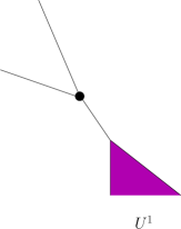
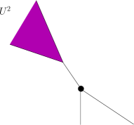
Figure 10: Placing the D3-branes at the north or south pole of the exceptional $\mathbb{CP}^{1}$ in the first small resolution gives VEVs to either the $U^{1}$ or $U^{2}$ baryons. These are related by the action of $SU(2)$.

All such points are equivalent under the $SU(2)$ isometry of the metric (4.1). By placing the $N$ D3-branes at the north (south) pole of $\mathbb{CP}^{1}=S^{2}$, the results of section 2.3 immediately imply that the only toric divisor that may produce a non-zero condensate is that shaded in Figure 10. This corresponds to the fields $U^{1}_{i}$ ($U^{2}_{i}$), where recall $i=1,\ldots,p$ labels the torsion line bundle. The theory should flow in the IR to the near horizon geometry of the $N$ D3-branes, which is determined by the toric diagrams in Figure 11. Indeed, according to our general discussion in section 2, this gravity solution should correspond to an RG flow from the $Y^{p,q}$ theory in the UV to the $\mathcal{N}=2$ $A_{p-1}$ SCFT orbifold theory in the IR, where the latter arises as the near horizon limit of the branes at the point $\mathbf{x}_{0}\in\mathbb{CP}^{1}$.

Figure 11: Toric diagrams for the $A_{p-1}=\mathbb{C}\times\mathbb{C}^{2}/\mathbb{Z}_{p}$ orbifold theories obtained by giving VEVs to the $U^{1}$ and $U^{2}$ baryons, respectively.

We now verify these facts directly in the gauge theory. In particular, we give non-zero VEVs to all $p$ of the $U^{1}$ fields by setting

$$U^{1}_{i}=\lambda_{i}\ \mathrm{I}_{N\times N}$$ (5.5)

where $\lambda_{i}\neq 0$ for $i=1,\ldots,p$. Each chiral matter field is in the bifundamental representation of $U(N)_{i}\times U(N)_{j}$ for the two nodes $i$ and $j$ that the corresponding arrow connects. The VEVs (5.5) then break the gauge symmetry to the diagonal $U(N)$ subgroup. This breaks the $U(N)^{2p}$ gauge symmetry to $U(N)^{p}$, where the nodes of the quiver are effectively contracted pairwise around the quiver diagram. The VEVs also break the $SU(2)$ flavour symmetry. The fields $U^{2}_{i}$ are adjoints under the diagonal $U(N)$, and thus become loops at each of the $p$ nodes. The superpotential becomes

$$\widetilde{W} = \sum_{i=1}^{q}\lambda_{i}V_{i}^{2}Y_{2i-1}-U_{i}^{2}V_{i}^{1}Y_{2i-1}+V_{i}^{1}U_{i+1}^{2}Y_{2i}-\lambda_{i+1}V_{i}^{2}Y_{2i}$$ (5.6)

$$+\sum_{i=q+1}^{p}\lambda_{i}Z_{i}U_{i+1}^{2}Y_{i+q}-\lambda_{i+1}Z_{i}Y_{i+q}U_{i}^{2}~{}.$$

Introducing the new fields

$$M_{i} = \lambda_{i}Y_{2i-1}-\lambda_{i+1}Y_{2i},\qquad i=1,\ldots,q$$ (5.7)

and substituting for $Y_{2i}$ in terms of $Y_{2i-1}$ one obtains

$$\widetilde{W} = \sum_{i=1}^{q}V_{i}^{2}M_{i}-U_{i}^{2}V_{i}^{1}Y_{2i-1}+\frac{1}{\lambda_{i+1}}V_{i}^{1}U_{i+1}^{2}(\lambda_{i}Y_{2i-1}-M_{i})$$ (5.8)

$$+\sum_{i=q+1}^{p}\lambda_{i}Z_{i}U_{i+1}^{2}Y_{i+q}-\lambda_{i+1}Z_{i}Y_{i+q}U_{i}^{2}~{}.$$

The quadratic terms give masses to the corresponding fields, which should thus be integrated out in the IR limit. Integrating out $V^{2}_{i}$ sets $M_{i}=0$ and hence

$$\lambda_{i}Y_{2i-1}=\lambda_{i+1}Y_{2i}\equiv\tilde{Y}_{i},\qquad i=1,\ldots,q~{}.$$ (5.9)

This reduces the number of $Y$ fields by $q$, giving $p$ $Y$ and $p$ $\tilde{Y}$ fields in total.

Figure 12: Quiver diagram for the $\mathbb{C}^{3}/\mathbb{Z}_{4}$ orbifold theory, obtained via Higgsing all $U^{1}$ or all $U^{2}$ baryons in the $Y^{4,1}$ theory. The origin of each field may be traced via its colour.

Integrating out $M_{i}$ sets $\lambda_{i}V_{i}^{2}=\lambda_{i+1}V_{i}^{1}U_{i+1}^{2}$. In the IR we thus obtain the effective superpotential

$$\widetilde{W}_{\mathrm{eff}}\ =\ \sum_{i=1}^{q}\frac{1}{\lambda_{i+1}}V_{i}^{1}U_{i+1}^{2}\tilde{Y}_{i}-\frac{1}{\lambda_{i}}U_{i}^{2}V_{i}^{1}\tilde{Y}_{i}+\sum_{i=q+1}^{p}\lambda_{i}Z_{i}U^{2}_{i+1}Y_{i+q}-\lambda_{i+1}Z_{i}Y_{i+q}U_{i}^{2}~{}.$$ (5.10)

This is precisely the matter content, and cubic superpotential, of the $\mathcal{N}=2$ $A_{p-1}$ orbifold theory. There are $p$ gauge groups $i=1,\ldots,p$, with the following matter content:

$U^{2}_{i}:$	$\mathrm{Ad}[U(N)_{i}]$,	$i=1,\ldots,p$
$V^{2}_{i}:$	$\overline{\mathbf{N}}_{i}\times\mathbf{N}_{i+1}$,	$i=1,\ldots,q$
$Z_{i}:$	$\overline{\mathbf{N}}_{i}\times\mathbf{N}_{i+1}$,	$i=q+1,\ldots,p$
$\tilde{Y}_{i}:$	$\overline{\mathbf{N}}_{i+1}\times\mathbf{N}_{i}$,	$i=1,\ldots,q$
${Y}_{i}:$	$\overline{\mathbf{N}}_{i-q+1}\times\mathbf{N}_{i-q}$,	$i=2q+1,\ldots,p+q$.

The final quiver for $Y^{4,1}$ is shown in Figure 12. Note that the couplings $\lambda_{i}$ may effectively all be set equal to one in (5.10) by the field redefinitions

$$U^{2}_{i} = \lambda_{i}\tilde{U}^{2}_{i},\qquad i=1,\ldots,p$$

$$Z_{i} = \frac{1}{\lambda_{i}\lambda_{i+1}}\tilde{Z}_{i},\quad i=q+1,\ldots,p+q~{}.$$ (5.11)

5.3 Small partial resolution II

In this section we consider the second small partial resolution. There are various inequivalent points $\mathbf{x}_{0}\in\mathbb{WCP}^{1}$ to place the $N$ D3-branes.

5.3.1 Higgsing $Z$

Consider first placing the $N$ D3-branes at the north pole of the exceptional $\mathbb{WCP}^{1}$, as shown in Figure 13.

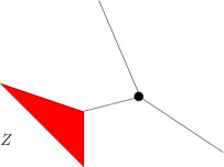
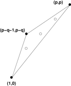
Figure 13: Placing the D3-branes at the north pole of the exceptional $\mathbb{WCP}^{1}$ in the second small partial resolution gives VEVs to all the $Z$ baryons.

This point has local geometry (tangent cone) $\mathbb{C}^{3}/\mathbb{Z}_{p+q}$, where recall from section 3.2.2 that the latter is embedded as $\mathbb{Z}_{p+q}\subset U(1)\subset SU(3)$ where the $U(1)$ subgroup has weights $(-2,1,1)$. According to our general discussion, the only fields that may acquire VEVs are the Z fields, and the theory should flow in the IR to the $\mathcal{N}=1$ orbifold theory corresponding to the abelian quotient singularity $\mathbb{C}^{3}/\mathbb{Z}_{p+q}$.

To verify the above directly in the gauge theory, we thus Higgs all $p-q$ of the $Z_{i}$ fields, $i=q+1,\ldots,p$, by setting

$$Z_{i}=\lambda_{i}\ \mathrm{I}_{N\times N}$$ (5.12)

where $\lambda_{i}\neq 0$ for $i=q+1,\ldots,p$. The Higgsing breaks to the diagonal $U(N)$ gauge groups: this contracts $p-q$ nodes in the quiver pairwise, leaving a $U(N)^{p+q}$ gauge theory. Of course, since $Z$ is a singlet under $SU(2)$, the VEVs preserve the $SU(2)$ symmetry. The cubic terms in the superpotential are unaffected. We obtain the superpotential

$$\widetilde{W}_{\mathrm{eff}}=\epsilon_{\alpha\beta}\sum_{i=1}^{q}U_{i}^{\alpha}V_{i}^{\beta}Y_{2i-1}+V_{i}^{\alpha}U_{i+1}^{\beta}Y_{2i}+\epsilon_{\alpha\beta}\sum_{i=q+1}^{p}\lambda_{i}U_{i+1}^{\alpha}{Y}_{i+q}U_{i}^{\beta}~{}.$$ (5.13)

Note that the couplings $\lambda_{i}$ may be effectively set to unity by the field redefinitions $\tilde{Y}_{i+q}=\lambda_{i}Y_{i+q}$, $i=q+1,\ldots,p$. This is indeed precisely the gauge theory for the $\mathcal{N}=1$ $\mathbb{C}^{3}/\mathbb{Z}_{p+q}$ orbifold singularity [12].

Figure 14: Quiver diagram for the $\mathbb{C}^{3}/\mathbb{Z}_{5}$ orbifold theory, obtained via Higgsing all $Z$ baryons in the $Y^{4,1}$ theory. The origin of each field may be traced via its colour.

5.3.2 Higgsing $Y$

Next consider placing the $N$ D3-branes at the south pole of the exceptional $\mathbb{WCP}^{1}$, as shown in Figure 15.

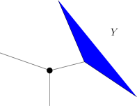
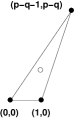
Figure 15: Placing the D3-branes at the south pole of the exceptional $\mathbb{WCP}^{1}$ in the second small partial resolution gives VEVs to all the $Y$ baryons.

This point has local geometry (tangent cone) $\mathbb{C}^{3}/\mathbb{Z}_{p-q}$, where again the latter is embedded as $\mathbb{Z}_{p-q}\subset U(1)\subset SU(3)$ where the $U(1)$ subgroup has weights $(-2,1,1)$. According to our general discussion, the only fields that may acquire VEVs are the $Y$ fields, and the theory should flow in the IR to the $\mathcal{N}=1$ orbifold theory corresponding to the abelian quotient singularity $\mathbb{C}^{3}/\mathbb{Z}_{p-q}$.

We thus Higgs all $p+q$ of the $Y_{i}$ fields, $i=1,\ldots,p+q$, by setting

$$Y_{i}=\lambda_{i}\ \mathrm{I}_{N\times N}$$ (5.14)

where $\lambda_{i}\neq 0$ for $i=1,\ldots,p+q$. This Higgsing leaves a $U(N)^{p-q}$ theory, one gauge group for each $Z$ field. Again the Higgsing leaves $SU(2)$ unbroken, resulting in the superpotential

$$\widetilde{W}=\epsilon_{\alpha\beta}\sum_{i=1}^{q}V_{i}^{\beta}\left(\lambda_{2i-1}U_{i}^{\alpha}-\lambda_{2i}U_{i+1}^{\alpha}\right)-\epsilon_{\alpha\beta}\sum_{i=q+1}^{p}\lambda_{i+q}Z_{i}U_{i+1}^{\alpha}U_{i}^{\beta}~{}.$$ (5.15)

We make the following field redefinition

$$M_{i}^{\alpha}=\lambda_{2i-1}U_{i}^{\alpha}-\lambda_{2i}U_{i+1}^{\alpha},\qquad i=1,\ldots,q$$ (5.16)

and solve for $U_{i+1}^{\alpha}$, for $i=1,\ldots,q$, in terms of $U_{1}^{\alpha}$ and $\{M_{i}^{\alpha}\}$. The first sum in (5.15) contains only quadratic terms, resulting in masses for these fields. In particular, integrating out $V_{i}^{\beta}$ sets $M_{i}^{\alpha}=0$ for all $i=1,\ldots,q$, resulting in

$$\lambda_{2i-1}U_{i}^{\alpha}=\lambda_{2i}U_{i+1}^{\alpha},\qquad i=1,\ldots,q~{}.$$ (5.17)

This leaves only $p-q$ independent $U^{\alpha}$ fields, for each $\alpha=1,2$. Integrating out $M_{i}^{\alpha}$ allows one to solve for the $V_{i}^{\beta}$. The IR superpotential is then

$$\widetilde{W}_{\mathrm{eff}}=\epsilon_{\alpha\beta}\sum_{i=q+1}^{p}\lambda_{i+q}{Z}_{i}U_{i+1}^{\alpha}U_{i}^{\beta}~{},$$ (5.18)

where as usual we may redefine $\tilde{Z}_{i}=\lambda_{i+q}Z_{i}$, $i=q+1,\ldots,p$ to set the coefficients equal to 1. This is the correct matter content and superpotential for the $\mathbb{C}^{3}/\mathbb{Z}_{p-q}$ orbifold theory.

Figure 16: Quiver diagram for the $\mathbb{C}^{3}$ theory (${\cal N}=4$ SYM), obtained via Higgsing all $Y$ baryons in the $Y^{4,3}$ theory. The origin of each field may be traced via its colour.

5.3.3 Higgsing $Z$ and $Y$

Finally, consider placing the D3-branes at a generic (non-singular) point on the exceptional $\mathbb{WCP}^{1}$, as shown in Figure 17. The near horizon limit of the branes depends on the parity of $p+q$: for $p+q$ even one obtains $\mathbb{C}\times\mathbb{C}^{2}/\mathbb{Z}_{2}$, whereas for $p+q$ odd one obtains $\mathbb{C}^{3}$. Thus this gravity solution describes an RG flow from the $Y^{p,q}$ theory in the UV to either the $\mathcal{N}=2$ $A_{1}$ orbifold theory, for $p+q$ even, or $\mathcal{N}=4$ SYM, for $p+q$ odd. Note that only in the former case is there an explicit Ricci-flat Kähler metric in section 4.

Figure 17: Placing the D3-branes at a generic point on the exceptional $\mathbb{WCP}^{1}$ of the second small resolution gives VEVs to all $Z$ and $Y$ baryons.

The picture in Figure 17 suggests that we Higgs all the $Z$ and $Y$ baryons simultaneously. We thus give the following non-zero VEVs:

$$Y_{i} = \lambda_{i}\ \mathrm{I}_{N\times N}+\tilde{Y}_{i}~{},\qquad i=1,\ldots,p+q$$

$$Z_{i} = \mu_{i}\ \mathrm{I}_{N\times N}+\tilde{Z}_{i}~{},\qquad i=q+1,\ldots,p~{}.$$ (5.19)

Notice that we have included explicitly the fluctuation fields around the vacuum expectation values.

Recalling that the quiver is in a toric phase where all loops corresponding to cubic and quartic superpotential terms appear consecutively on going around the quiver, one can verify that starting from any node of the quiver, and grouping it with gauge groups (nodes) connected to the first one by a Higgsed field ($Z$ or $Y$), there are two possibilities: (1) if $p+q$ is even, the nodes are divided into two disjoint sets of $p$ gauge groups each, and therefore the unbroken gauge groups are the two diagonal subgroups respectively, which we denote $U(N)_{1}\times U(N)_{2}$, (2) if $p+q$ is odd, chasing around the quiver the nodes that are connected by fields that have a non-zero VEV, we see that all nodes are covered. Thus the unbroken gauge group is simply the diagonal $U(N)_{\mathrm{diag}}$.

Most of the calculation of the effective IR superpotential may be carried out for the two cases simultaneously, and we will indicate at which point the two calculations differ. Inserting (5.19) into the superpotential one obtains

$$\widetilde{W} = \epsilon_{\alpha\beta}\sum_{i=1}^{q}V_{i}^{\beta}(\lambda_{2i-1}U_{i}^{\alpha}-\lambda_{2i}U_{i+1}^{\alpha})-\epsilon_{\alpha\beta}\sum_{i=q+1}^{p}\mu_{i}\lambda_{i+q}U_{i+1}^{\alpha}U_{i}^{\beta}$$ (5.20)

$$+ \epsilon_{\alpha\beta}\sum_{i=1}^{q}\left(U_{i}^{\alpha}V_{i}^{\beta}\tilde{Y}_{2i-1}+V_{i}^{\alpha}U_{i+1}^{\beta}\tilde{Y}_{2i}\right)$$

$$- \epsilon_{\alpha\beta}\sum_{i=q+1}^{p}\left(\mu_{i}U^{\alpha}_{i+1}U_{i}^{\beta}\tilde{Z}_{i}+\lambda_{i+q}U^{\beta}_{i}U_{i+1}^{\alpha}\tilde{Y}_{i+q}\right)~{},$$

where we have omitted the quartic terms that will turn out to be irrelevant in the IR. The first line is quadratic in the $2(p+q)$ fields $U$ and $V$; however, not all these fields get masses. To see how many of them remain massless one must diagonalise the $2(p+q)\times 2(p+q)$ quadratic form in the $U$ and $V$ fields. It turns out that four linear combinations are massless if $p+q$ is even, whereas only two combinations are massless if $p+q$ is odd. We may set $M_{i}^{\alpha}=\lambda_{2i-1}U_{i}^{\alpha}-\lambda_{2i}U_{i+1}^{\alpha}$ for $i=1,\ldots,q$, and go to the basis consisting of $M_{i}^{\alpha},V_{i}^{\alpha}$ for $i=1,\dots,q$, and $U_{q+2}^{\alpha},\dots,U_{p}^{\alpha},U_{1}^{\alpha}$, where we have solved for $U_{q+1}^{\alpha}$ in terms of the other fields as

$$U_{q+1}^{\alpha} = cU_{1}^{\alpha}-\sum_{i=1}^{q}a_{i}M_{i}^{\alpha}~{}.$$ (5.21)

Integrating out $V_{i}^{\alpha}$ and $M_{i}^{\alpha}$ then implies

$$\begin{array}[]{rcl}\lambda_{2i-1}U_{i}^{\alpha}&=&\lambda_{2i}U_{i+1}^{\alpha}\\[4.2679pt] V_{i}^{\alpha}/a_{i}&=&\lambda_{2q+1}\mu_{q+1}U_{q+2}^{\alpha}\end{array}\qquad i=1,\dots,q~{},$$ (5.24)

respectively. Integrating out the remaining $U^{\alpha}_{i}$ fields yields

$$\mu_{i-1}\lambda_{q+i-1}U^{\alpha}_{i-1} = \mu_{i}\lambda_{i+q}U^{\alpha}_{i+1}\qquad i=q+2,\dots,p$$ (5.25)

$$\mu_{p}\lambda_{p+q}U^{\alpha}_{p} = c\mu_{q+1}\lambda_{2q+1}U^{\alpha}_{q+2}\qquad(i=1)~{}.$$ (5.26)

If $p+q$ is even we obtain the following identifications:

$$A^{\alpha}=\frac{U_{1}^{\alpha}}{c_{1}}=\dots=\frac{U_{q}^{\alpha}}{c_{q}}=\frac{U_{q+1}^{\alpha}}{c_{q+1}}=\dots=\frac{U_{p-1}^{\alpha}}{c_{p-1}} \in \mathbf{\overline{N}}_{1}\times\mathbf{N}_{2}~{}{\;\;}$$

$$B^{\alpha}=\frac{V_{1}^{\alpha}}{a_{1}}=\dots=\frac{V_{q}^{\alpha}}{a_{q}}=\frac{U_{q+2}^{\alpha}}{c_{q+2}}=\dots=\frac{U^{\alpha}_{p}}{c_{p}} \in \mathbf{N}_{1}\times\mathbf{\overline{N}}_{2}~{},$$ (5.27)

where $c_{i}$ are constants that may be determined iteratively using the relations (5.24) - (5.26). Inserting these into $\widetilde{W}$, we get the final expression for the effective superpotential

$$\widetilde{W}_{\mathrm{eff}} = \tilde{H}_{1}\left(A^{1}B^{2}-A^{2}B^{1}\right)+\tilde{H}_{2}\left(B^{1}A^{2}-B^{2}A^{1}\right)$$ (5.28)

where we have defined the two adjoint fields

$$\tilde{H}_{1} = \sum_{i=1}^{q}a_{i}c_{i}\tilde{Y}_{2i-1}+\sum_{i=1}^{(p-q)/2}c_{q+2i-1}c_{q+2i}\left(\lambda_{2q+2i-1}\tilde{Y}_{2q+2i-1}-\mu_{q+2i-1}\tilde{Z}_{q+2i-1}\right)$$

$$\tilde{H}_{2} = \sum_{i=1}^{q}a_{i}c_{i}\tilde{Y}_{2i}+\sum_{i=1}^{(p-q)/2}c_{q+2i}c_{q+2i+1}\left(\lambda_{2q+2i}\tilde{Y}_{2q+2i}-\mu_{q+2i}\tilde{Z}_{q+2i}\right)~{}.$$ (5.29)

This is indeed the correct superpotential for the ${\cal N}=2$ $A_{1}$ theory, as pictured in Figure 18.

Figure 18: Quiver diagram for the $A_{1}$ theory, obtained via Higgsing all $Z$ and $Y$ baryons in a $Y^{p,q}$ theory with $p+q$ even. Bifundamentals arise as a mixture of $U$ and $V$ fields, while the adjoints arise as a combination of $Z$ and $Y$ fields.

If $p+q$ is odd, the last entries in the relations (5.27) are exchanged, hence $U^{\alpha}_{p}\sim U^{\alpha}_{q+1}$ and $U^{\alpha}_{p-1}\sim U^{\alpha}_{q+2}$, so that all fields get identified on using (5.26). This case may be obtained formally from the result above, on setting $X^{\alpha}=A^{\alpha}=B^{\alpha}$ and inserting this into (5.28). Of course, one has to remember that the gauge group is broken further to the diagonal $U(N)_{\mathrm{diag}}$. The final expression for the effective superpotential is simply

$$\widetilde{W}_{\mathrm{eff}} = \tilde{H}(X^{1}X^{2}-X^{2}X^{1})~{},$$ (5.30)

where $\tilde{H}=\tilde{H}_{1}+\tilde{H}_{2}$. This is the ${\cal N}=4$ SYM theory, as expected.

5.4 Canonical partial resolutions

Finally, we consider the canonical partial resolutions of section 3.3. These correspond to blowing up a toric Fano orbifold $M$. The partial resolution is the total space of the canonical orbifold line bundle over this Fano orbifold. There are $p-1$ such partial resolutions, labelled naturally by an integer $s$, with $0<s<p$, that labels the blow-up vertex in the toric diagram – see Figure 1. In this section we consider placing the $N$ D3-branes at the toric fixed points of the exceptional divisor. As one can see from Figure 4, there are four such points. However, two points that lie on the same $\mathbb{CP}^{1}\subset M$ divisor in $M$ are related by the isometric action of $SU(2)$. Thus there are really only two cases to consider. We consider these in the next two subsections.

5.4.1 Higgsing $U^{1}$, $V^{1}$ and $Z$

Placing the D3-branes at the corner of the exceptional divisor $M$, as in Figure 19, implies that no $Y$ or $U^{2}$ fields get non-zero VEVs. In this section we show that a certain two-parameter family of VEVs all flow to the same IR theory, namely the $\mathcal{N}=2$ $A_{p-s-1}$ orbifold theory. This is precisely as expected from the gravity dual, since this is indeed the near-horizon geometry of the stack of D3-branes.

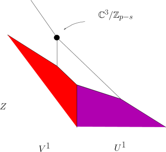
Figure 19: Placing the D3-branes at the $U(1)^{3}$-invariant point on the exceptional divisor, as shown, gives VEVs to a set of $U^{1}$, $V^{1}$ and $Z$ baryons.

We give the following VEVs:

$$U^{1}_{i} = \lambda_{i}\ \mathrm{I}_{N\times N},\qquad i=1,\ldots,p$$

$$V^{1}_{i} = \mu_{i}\ \mathrm{I}_{N\times N},\qquad i=1,\ldots t$$

$$Z_{i} = \mu_{i}\ \mathrm{I}_{N\times N},\qquad i=q+1,\ldots,q+s-t~{}.$$ (5.31)

This is not the most general set of VEVs we could turn on, but an analysis of the most general case would be too cumbersome; the above choice for the VEVs is nonetheless still rather general. Here $0\leq t\leq s$, with $0<s<p$. We also assume, again for simplicity, that $t<q$ and $s-t<p-q$; the non-strict forms of these inequalities must hold, since e.g. there are only $q$ $V^{1}$ fields to give VEVs to. The strict inequalities slightly simplify some of the following analysis.

The superpotential becomes

$$\widetilde{W} = \sum_{i=1}^{t}\lambda_{i}V_{i}^{2}Y_{2i-1}-\mu_{i}U_{i}^{2}Y_{2i-1}+\mu_{i}U_{i+1}^{2}Y_{2i}-\lambda_{i+1}V_{i}^{2}Y_{2i}$$ (5.32)

$$+ \sum_{i=t+1}^{q}\lambda_{i}V_{i}^{2}Y_{2i-1}-U_{i}^{2}V_{i}^{1}Y_{2i-1}+V_{i}^{1}U_{i+1}^{2}Y_{2i}-\lambda_{i+1}V_{i}^{2}Y_{2i}$$

$$+ \sum_{i=q+1}^{q+s-t}\lambda_{i}\mu_{i}U_{i+1}^{2}Y_{i+q}-\lambda_{i+1}\mu_{i}U_{i}^{2}Y_{i+q}$$

$$+ \sum_{i=q+1+s-t}^{p}\lambda_{i}Z_{i}U_{i+1}^{2}Y_{i+q}-\lambda_{i+1}Z_{i}Y_{i+q}U_{i}^{2}~{}.$$

We introduce the following new fields

$$M_{i} = \lambda_{i}Y_{2i-1}-\lambda_{i+1}Y_{2i},\qquad i=1,\ldots,q$$

$$N_{i} = \mu_{i}Y_{2i}-\mu_{i+1}Y_{2i+1},\qquad i=1,\ldots,t-1$$

$$P_{i} = \mu_{i}\left(\lambda_{i}U_{i+1}^{2}-\lambda_{i+1}U_{i}^{2}\right),\qquad i=q+1,\ldots,q+s-t$$ (5.33)

and substitute for $Y_{2i}$ in terms of $Y_{2i-1}$ and $M_{i}$, $i=1,\ldots,q$; $Y_{2i+1}$ in terms of $Y_{2i}$ and $N_{i}$, $i=1,\ldots,t-1$; and $U_{i+1}^{2}$ in terms of $U_{i}^{2}$ and $P_{i}$, $i=q+1,\ldots,q+s-t$. In particular, note that

$$Y_{2t-1}=cY_{1}-\sum_{i=1}^{t-1}a_{i}M_{i}+b_{i}N_{i}$$ (5.34)

where $c$, $a_{i}$ and $b_{i}$ are positive constants that we do not need to determine explicitly. The superpotential, in these new variables, then reads

$$\widetilde{W} = -\lambda_{1}U_{1}^{2}Y_{1}+\left(\sum_{i=1}^{t-1}V_{i}^{2}M_{i}+U_{i+1}^{2}N_{i}\right)+V_{t}^{2}M_{t}+\frac{1}{\lambda_{t+1}}\mu_{t}U_{t+1}^{2}\left(\lambda_{t}Y_{2t-1}-M_{t}\right)$$ (5.35)

$$+ \sum_{i=t+1}^{q}V_{i}^{2}M_{i}-U_{i}^{2}V_{i}^{1}Y_{2i-1}+\frac{1}{\lambda_{i+1}}V_{i}^{1}U_{i+1}^{2}\left(\lambda_{i}Y_{2i-1}-M_{i}\right)+\sum_{i=q+1}^{q+s-t}Y_{i+q}P_{i}$$

$$+ \sum_{i=q+1+s-t}^{p}\lambda_{i}Z_{i}U_{i+1}^{2}Y_{i+q}-\lambda_{i+1}Z_{i}Y_{i+q}U_{i}^{2}$$

where one must substitute for $Y_{2t-1}$ in the first line using (5.34). As usual, the quadratic terms lead to masses for the corresponding fields, which must then be integrated out in the IR. Integrating out $V_{i}^{2}$, $U_{i+1}^{2}$ and $Y_{i+q}$ sets

$$M_{i} = 0,\qquad i=1,\ldots,q$$

$$N_{i} = 0,\qquad i=1,\ldots,t-1$$

$$P_{i} = 0,\qquad i=q+1,\ldots,q+s-t$$ (5.36)

respectively. Integrating out $M_{i}$, $i=1,\ldots,t-1$ sets $V_{i}^{2}=(a_{i}\lambda_{t}\mu_{t}/\lambda_{t+1})U_{t+1}^{2}$. Integrating out $M_{t}$ sets $V_{t}^{2}=(\mu_{t}/\lambda_{t+1})U_{t+1}^{2}$. Integrating out $M_{i}$, $i=t+1,\ldots,q$ sets $\lambda_{i+1}V_{i}^{2}=V_{i}^{1}U_{i+1}^{2}$. Integrating out $N_{i}$, $i=1,\ldots,t-1$ sets $U_{i+1}^{2}=(b_{i}\lambda_{t}\mu_{t}/\lambda_{t+1})U_{t+1}^{2}$. Integrating out $P_{i}$, $i=q+1,\ldots,q+1+s-t$ sets $Y_{i+q}=0$.

Finally, we integrate out $U_{1}^{2}$ to obtain $\lambda_{1}Y_{1}=\lambda_{p}Y_{p+q}Z_{p}$; $Y_{1}$ to obtain

$$\lambda_{1}U_{1}^{2}=(c\lambda_{t}\mu_{t}/\lambda_{t+1})U_{t+1}^{2}~{};$$ (5.37)

and $U_{t+1}^{2}$ to obtain $\mu_{t}\lambda_{t}Y_{2t-1}=\lambda_{t+1}V_{t+1}^{1}Y_{2t+1}$.

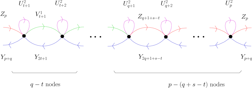
Figure 20: Quiver for the $\mathcal{N}=2$ $A_{p-s-1}$ orbifold quiver gauge theory, obtained via Higgsing a set of $U^{1}$, $V^{1}$ and $Z$ fields.

All this results in the simple cubic superpotential

$$\widetilde{W}_{\mathrm{eff}} = \sum_{i=t+1}^{q}\frac{\lambda_{i}}{\lambda_{i+1}}V_{i}^{1}U_{i+1}^{2}Y_{2i-1}-U_{i}^{2}V_{i}^{1}Y_{2i-1}$$ (5.38)

$$+ \sum_{i=q+1+s-t}^{p}\lambda_{i}Z_{i}U_{i+1}^{2}Y_{i+q}-\lambda_{i+1}Z_{i}Y_{i+q}U_{i}^{2}~{}.$$

Here $U_{t+1}^{2}$ is to be identified with $U_{1}^{2}=U_{p+1}^{2}$ via (5.37), and $U_{q+1+s-t}^{2}$ is to be identified with $U_{q+1}^{2}$ using $P_{i}=0$ iteratively in the relations (5.4.1). As usual, the reader may check that some simple field redefinitions effectively set all the constants in $\widetilde{W}_{\mathrm{eff}}$ equal to one. This is precisely the field content and superpotential of the $\mathcal{N}=2$ $A_{p-s-1}$ orbifold theory, depicted in Figure 20.

5.4.2 Higgsing $U^{1}$ and $Y$

Placing the D3-branes at the corner of the exceptional divisor $M$, as in Figure 21, implies that no $Z$ or $U^{2}$ fields get non-zero VEVs. In this section we show that a certain two-parameter family of VEVs all flow to the same IR theory, namely the $\mathcal{N}=2$ $A_{p-r-1}$ orbifold theory. Recall that here $r=p-s$. This is again precisely as expected from the gravity dual, since this is indeed the near-horizon geometry of the stack of D3-branes.

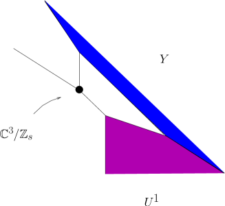
Figure 21: Placing the D3-branes at the $U(1)^{3}$-invariant point on the exceptional divisor, as shown, gives VEVs to a set of $U^{1}$ and $Y$ baryons.

We give the following VEVs:

$$U^{1}_{i} = \lambda_{i}\ \mathrm{I}_{N\times N},\qquad i=1,\ldots,p$$

$$Y_{i} = \mu_{i}\ \mathrm{I}_{N\times N},\qquad i=1,\ldots 2t$$

$$Y_{i} = \mu_{i}\ \mathrm{I}_{N\times N},\qquad i=2q+1,\ldots,2q+r-t~{}.$$ (5.39)

Again, this is not the most general set of VEVs we could turn on, but rather a representative calculation. In particular, one may also turn on an odd number of VEVs for the cubic $Y$ fields. We have $0\leq t\leq r$, with $0<r<p$, $t<q$, $r-t<p-q$.

The superpotential becomes

$$\widetilde{W}_{\mathrm{eff}} = \sum_{i=1}^{t}\lambda_{i}\mu_{2i-1}V_{i}^{2}-\mu_{2i-1}V_{i}^{1}U_{i}^{2}+\mu_{2i}V_{i}^{1}U_{i+1}^{2}-\lambda_{i+1}\mu_{2i}V_{i}^{2}$$ (5.40)

$$+ \sum_{i=t+1}^{q}\lambda_{i}V_{i}^{2}Y_{2i-1}-U_{i}^{2}V_{i}^{1}Y_{2i-1}+V_{i}^{1}U_{i+1}^{2}Y_{2i}-\lambda_{i+1}V_{i}^{2}Y_{2i}$$

$$+ \sum_{i=q+1}^{q+r-t}\lambda_{i}\mu_{i+q}Z_{i}U_{i+1}^{2}-\lambda_{i+1}\mu_{i+q}Z_{i}U_{i}^{2}$$

$$+ \sum_{i=q+1+r-t}^{p}\lambda_{i}Z_{i}U_{i+1}^{2}Y_{i+q}-\lambda_{i+1}Z_{i}Y_{i+q}U_{i}^{2}~{}.$$

Note the linear terms in $V_{i}^{2}$ for $i=1,\ldots,2t$. Strictly speaking we should have allowed for fluctuations of the fields around their vacuum expectation values. These fluctuations will give a mass to $V_{i}^{2}$, which as usual is then integrated out in the IR. Since these fluctuation terms will turn out to be irrelevant in the IR, we suppress them in order to keep expressions to a manageable length. We now define

$$M_{i} = \mu_{2i}U_{i+1}^{2}-\mu_{2i-1}U_{i}^{2}\qquad i=1,\ldots,2t$$

$$N_{i} = \lambda_{i}Y_{2i-1}-\lambda_{i+1}Y_{2i},\qquad i=t+1,\ldots,q$$

$$P_{i} = \mu_{i+q}\left(\lambda_{i}U_{i+1}^{2}-\lambda_{i+1}U_{i}^{2}\right),\qquad i=q+1,\ldots,q+r-t~{}.$$ (5.41)

We then substitute for $U_{i+1}^{2}$ in terms of $U_{i}^{2}$ and $M_{i}$, $i=1,\ldots,2t$; $Y_{2i}$ in terms of $Y_{2i-1}$ and $N_{i}$, $i=t+1,\ldots,q$; and $U_{i+1}^{2}$ in terms of $U_{i}^{2}$ and $P_{i}$, $i=q+1,\ldots,q+r-t$. Integrating out massive fields proceeds much as in the previous subsection. In particular, however, we obtain the necessary relations

$$\lambda_{i}\mu_{2i-1}=\lambda_{i+1}\mu_{2i},\qquad i=1,\ldots,t$$ (5.42)

on the VEVs. These effectively come from the F-term relations. There are thus effectively only $r$ independent VEVs for the $Y$ fields, rather than the $2t+(r-t)$ VEVs we began with. The pattern of VEVs then parallels that for the $Z$ fields in the previous subsection. The final effective superpotential in the IR is given by

$$\widetilde{W}_{\mathrm{eff}} = \sum_{i=t+1}^{q}\frac{\lambda_{i}}{\lambda_{i+1}}V_{i}^{1}U_{i+1}^{2}Y_{2i-1}-U_{i}^{2}V_{i}^{1}Y_{2i-1}$$ (5.43)

$$+ \sum_{i=q+1+r-t}^{p}\lambda_{i}Z_{i}U_{i+1}^{2}Y_{i+q}-\lambda_{i+1}Z_{i}Y_{i+q}U_{i}^{2}~{}.$$

Here $U_{t+1}^{2}$ is essentially identified with $U_{1}^{2}$; and $U_{q+1+r-t}^{2}$ is essentially identified with $U_{q+1}^{2}$. Note this is precisely the same as (5.38), with $r$ in place of $s$. This is therefore the matter content and cubic superpotential of the $A_{p-r-1}$ orbifold quiver gauge theory.

6 Discussion

In this paper we studied deformations of SCFTs with Sasaki-Einstein duals, obtained by giving non-zero VEVs to baryonic operators. We have argued that giving expectation values to baryonic operators (and only to these) in a superconformal quiver induces an RG flow to another IR conformal fixed point. The supergravity backgrounds AdS/CFT dual to these flows are warped resolved asymptotically conical Calabi-Yau metrics, where the warping is induced by a stack of $N$ D3-branes placed at some residual singularity, encoding the IR SCFT. When the geometries and field theories are toric, one may represent the full background in terms of pq-web-like diagrams. As explicit examples, we have discussed the partially resolved $Y^{p,q}$ metrics presented in [26]. The toric geometry description of the latter elucidates the dual field theory interpretation in terms of VEVs of baryonic operators.

We have also discussed a proposal for computing the condensate of the baryonic operators that are turned on in a given VEV-induced RG flow. In particular, we have given further evidence for identifying the exponentiated on-shell Euclidean D3-brane action as the string dual to baryonic condensates in a generic supergravity background of the above type. This identification gives a simple sufficient condition for a condensate to vanish, and we have checked this criterion in a number of non-trivial examples. However, the examples studied in this paper make clear that in a generic situation (i.e different from the conifold example discussed in [20]) the calculation of the condensate that we have outlined is necessarily rather more complicated. Indeed, recall that the AdS/CFT definition of a baryonic particle involves specifying a supersymmetric 3-submanifold and a flat (hence torsion) line bundle. Incorporating this into the instantonic D3-brane calculation requires studying the extension of this pair of data from the boundary to the interior. In turn, this requires a careful analysis of the flat background fields in a given geometry. These issues will be addressed in future work [36].

Acknowledgments

We would like to thank I. Klebanov, J. Maldacena, A. Murugan, Y. Tachikawa and S.-T. Yau for useful discussions. The research of J. F. S. at the University of Oxford is supported by a Royal Society University Research Fellowship, although the majority of this work was carried out at Harvard University, supported by NSF grants DMS-0244464, DMS-0074329 and DMS-9803347. D. M. would like to thank the physics and mathematics departments of Harvard University for hospitality during the early stages of this work. He acknowledges support from NSF grant PHY-0503584.

References

- [1] J. M. Maldacena, “The large N limit of superconformal field theories and supergravity,” Adv. Theor. Math. Phys. 2, 231 (1998) [Int. J. Theor. Phys. 38, 1113 (1999)] [arXiv:hep-th/9711200].
- [2] A. Kehagias, “New type IIB vacua and their F-theory interpretation,” Phys. Lett. B 435, 337 (1998) [arXiv:hep-th/9805131].
- [3] I. R. Klebanov and E. Witten, “Superconformal field theory on threebranes at a Calabi-Yau singularity,” Nucl. Phys. B 536, 199 (1998) [arXiv:hep-th/9807080].
- [4] B. S. Acharya, J. M. Figueroa-O’Farrill, C. M. Hull and B. J. Spence, “Branes at conical singularities and holography,” Adv. Theor. Math. Phys. 2, 1249 (1999) [arXiv:hep-th/9808014].
- [5] D. R. Morrison and M. R. Plesser, “Non-spherical horizons. I,” Adv. Theor. Math. Phys. 3, 1 (1999) [arXiv:hep-th/9810201].
- [6] J. P. Gauntlett, D. Martelli, J. Sparks and D. Waldram, “Supersymmetric AdS5 solutions of M-theory,” Class. Quant. Grav. 21, 4335 (2004) [arXiv:hep-th/0402153].
- [7] J. P. Gauntlett, D. Martelli, J. Sparks and D. Waldram, “Sasaki-Einstein metrics on ,” Adv. Theor. Math. Phys. 8, 711 (2004) [arXiv:hep-th/0403002].
- [8] M. Cvetic, H. Lu, D. N. Page and C. N. Pope, “New Einstein-Sasaki and Einstein spaces from Kerr-de Sitter,” [arXiv:hep-th/0505223].
- [9] D. Martelli and J. Sparks, “Toric Sasaki-Einstein metrics on ,” Phys. Lett. B 621, 208 (2005) [arXiv:hep-th/0505027].
- [10] D. Martelli and J. Sparks, “Toric geometry, Sasaki-Einstein manifolds and a new infinite class of AdS/CFT duals,” Commun. Math. Phys. 262, 51 (2006) [arXiv:hep-th/0411238].
- [11] M. Bertolini, F. Bigazzi and A. L. Cotrone, “New checks and subtleties for AdS/CFT and -maximization,” JHEP 0412, 024 (2004) [arXiv:hep-th/0411249].
- [12] S. Benvenuti, S. Franco, A. Hanany, D. Martelli and J. Sparks, “An infinite family of superconformal quiver gauge theories with Sasaki-Einstein duals,” JHEP 0506 (2005) 064 [arXiv:hep-th/0411264].
- [13] S. Benvenuti and M. Kruczenski, “From Sasaki-Einstein spaces to quivers via BPS geodesics: ,” JHEP 0604, 033 (2006) [arXiv:hep-th/0505206].
- [14] S. Franco, A. Hanany, D. Martelli, J. Sparks, D. Vegh and B. Wecht, “Gauge theories from toric geometry and brane tilings,” JHEP 0601, 128 (2006) [arXiv:hep-th/0505211].
- [15] A. Butti, D. Forcella and A. Zaffaroni, “The dual superconformal theory for manifolds,” JHEP 0509, 018 (2005) [arXiv:hep-th/0505220].
- [16] I. R. Klebanov and E. Witten, “AdS/CFT correspondence and symmetry breaking,” Nucl. Phys. B 556, 89 (1999) [arXiv:hep-th/9905104].
-
[17]
S. Benvenuti, M. Mahato, L. A. Pando Zayas and Y. Tachikawa,
“The gauge/gravity theory of blown up four cycles,” [arXiv:hep-th/0512061]. - [18] W. Chen, M. Cvetic, H. Lu, C. N. Pope and J. F. Vazquez-Poritz, “Resolved Calabi-Yau Cones and Flows from Superconformal Field Theories,” Nucl. Phys. B 785, 74 (2007) [arXiv:hep-th/0701082].
-
[19]
M. Cvetic and J. F. Vazquez-Poritz,
“Warped Resolved Cones,”
arXiv:0705.3847 [hep-th]. - [20] I. R. Klebanov and A. Murugan, “Gauge/gravity duality and warped resolved conifold,” JHEP 0703, 042 (2007) [arXiv:hep-th/0701064].
- [21] A. Butti, M. Grana, R. Minasian, M. Petrini and A. Zaffaroni, “The baryonic branch of Klebanov-Strassler solution: A supersymmetric family of structure backgrounds,” JHEP 0503, 069 (2005) [arXiv:hep-th/0412187].
- [22] A. Dymarsky, I. R. Klebanov and N. Seiberg, “On the moduli space of the cascading gauge theory,” JHEP 0601, 155 (2006) [arXiv:hep-th/0511254].
- [23] L. A. Pando Zayas and A. A. Tseytlin, “3-branes on spaces with topology,” Phys. Rev. D 63, 086006 (2001) [arXiv:hep-th/0101043].
- [24] L. Bérard-Bergery, “Sur de nouvelles variétés riemanniennes d’Einstein,” Institut Elie Cartan 6, 1 (1982).
- [25] D. N. Page and C. N. Pope, “Inhomogeneous Einstein Metrics On Complex Line Bundles,” Class. Quant. Grav. 4, 213 (1987).
- [26] D. Martelli and J. Sparks, “Resolutions of non-regular Ricci-flat Kähler cones,” arXiv:0707.1674 [math.DG].
- [27] T. Oota and Y. Yasui, “Explicit toric metric on resolved Calabi-Yau cone,” Phys. Lett. B 639, 54 (2006), [arXiv:hep-th/0605129].
- [28] H. Lu and C. N. Pope, “Resolutions of cones over Einstein-Sasaki spaces,” Nucl. Phys. B 782, 171 (2007) [arXiv:hep-th/0605222].
- [29] A. K. Balasubramanian, S. Govindarajan and C. N. Gowdigere, “Symplectic potentials and resolved Ricci-flat ACG metrics,” Class. Quant. Grav. 24, 6393 (2007) [arXiv:0707.4306 [hep-th]].
- [30] N. Th. Varopoulos, “Green’s functions on positively curved manifolds,” J. Funct. Anal. 45 (1982), no. 1, 109-118.
- [31] E. Witten, “Baryons and branes in anti de Sitter space,” JHEP 9807, 006 (1998) [arXiv:hep-th/9805112].
- [32] S. Gukov, M. Rangamani and E. Witten, “Dibaryons, strings, and branes in AdS orbifold models,” JHEP 9812, 025 (1998) [arXiv:hep-th/9811048].
- [33] D. Berenstein, C. P. Herzog and I. R. Klebanov, “Baryon spectra and AdS/CFT correspondence,” JHEP 0206, 047 (2002) [arXiv:hep-th/0202150].
- [34] S. J. Rey and J. T. Yee, “Macroscopic strings as heavy quarks in large N gauge theory and anti-de Sitter supergravity,” Eur. Phys. J. C 22, 379 (2001) [arXiv:hep-th/9803001].
- [35] J. M. Maldacena, “Wilson loops in large field theories,” Phys. Rev. Lett. 80, 4859 (1998) [arXiv:hep-th/9803002].
- [36] D. Martelli and J. Sparks, “Symmetry-breaking vacua and baryon condensates in AdS/CFT,” to appear.
- [37] A. Karch, A. O’Bannon and K. Skenderis, “Holographic renormalization of probe D-branes in AdS/CFT,” JHEP 0604, 015 (2006) [arXiv:hep-th/0512125].
- [38] S. S. Gubser, I. R. Klebanov and A. M. Polyakov, “Gauge theory correlators from non-critical string theory,” Phys. Lett. B 428, 105 (1998) [arXiv:hep-th/9802109].
- [39] E. Witten, “Anti-de Sitter space and holography,” Adv. Theor. Math. Phys. 2, 253 (1998) [arXiv:hep-th/9802150].
- [40] M. K. Benna, A. Dymarsky and I. R. Klebanov, “Baryonic condensates on the conifold,” JHEP 0708, 034 (2007) [arXiv:hep-th/0612136].
- [41] C. V. Johnson, “D-brane primer,” [arXiv:hep-th/0007170].
- [42] M. Atiyah and E. Witten, “M-theory dynamics on a manifold of G(2) holonomy,” Adv. Theor. Math. Phys. 6, 1 (2003) [arXiv:hep-th/0107177].
- [43] H. Kihara, M. Sakaguchi and Y. Yasui, “Scalar Laplacian on Sasaki-Einstein manifolds ,” Phys. Lett. B 621, 288 (2005) [arXiv:hep-th/0505259].
- [44] S. Benvenuti, A. Hanany and P. Kazakopoulos, “The toric phases of the quivers,” JHEP 0507, 021 (2005) [arXiv:hep-th/0412279].