USING INVARIANTS FOR PHYLOGENETIC TREE CONSTRUCTION

Abstract

Phylogenetic invariants are certain polynomials in the joint probability distribution of a Markov model on a phylogenetic tree. Such polynomials are of theoretical interest in the field of algebraic statistics and they are also of practical interest—they can be used to construct phylogenetic trees. This paper is a self-contained introduction to the algebraic, statistical, and computational challenges involved in the practical use of phylogenetic invariants. We survey the relevant literature and provide some partial answers and many open problems.

92B10, 92D15, 13P10, 05C05

1 Introduction

The emerging field of algebraic statistics (cf. [42]) has at its core the belief that many statistical problems are inherently algebraic. Statistical problems are often analyzed by specifying a model—a family of possible probability distributions to explain the data. In particular, many statistical models are defined parametrically by polynomials and thus involve algebraic varieties. From this point of view, one would hope that the ideal of polynomials that vanish on a statistical model would give statistical information about the model. This is not a new idea in statistics, indeed, tests based on polynomials that vanish on a model include the odds-ratio, which is based on the determinant of a two by two matrix. The polynomials that vanish on the statistical model have come to be known as the (algebraic) invariants of the model.

The field of phylogenetics provides important statistical and biological models with interesting combinatorial structure. The central problem in phylogenetics is to determine the evolutionary relationships among a set of taxa (short for taxonomic units, which could be species, for example). To a first approximation, these relationships can be represented using rooted binary trees, where the leaves correspond to the observed taxa and the interior nodes to ancestors. For example, Figure 1 shows the relationships between a portion of a gene in seven mammalian species.

Phylogenetic invariants are polynomials in the joint probability distribution describing sequence data that vanish on distributions arising from a particular tree and model of sequence evolution. The first of the invariants for phylogenetic tree models were discovered by Lake and Cavender-Felsenstein [36, 14]. This set off a flurry of work: in mathematics, generalizing these invariants (cf. [27, 21, 52]) and in phylogenetics, using these invariants to construct trees (cf. [29, 38, 39, 44, 45]). However, the linear invariants didn’t fare well in simulations [30] and the idea fell into disuse.

However, the study of phylogenetic invariants was revived in the field of algebraic statistics; the subsequent theoretical (cf. [2, 50, 12, 5]) and practical (cf. [13, 11, 18, 20, 34]) developments have given cause for optimism in using invariants to construct phylogenetic trees. There are benefits to these algebraic tools; however, obstacles in algebraic geometry, statistics, and computer science must be overcome if they are to live up to their potential. In this paper, we formulate and analyze some of the fundamental advantages and difficulties in using algebraic statistics to construct phylogenetic trees, describing the current research and formulating many open problems.

In geometric terms, the problem of phylogenetic tree construction can be stated as follows. We observe DNA sequences from $n$ different taxa and wish to determine which binary tree with $n$ leaves best describes the relationships between these sequences for a fixed model of evolution. Each of these trees corresponds to a different algebraic variety in $\mathbb{R}^{4^{n}}$. The DNA sequences correspond to a certain point in $\mathbb{R}^{4^{n}}$ as well. Picking the best tree means picking the variety that is closest to the data point in some sense. Since the data will not typically lie on the variety of any tree, we have to decide what is meant by “close”.

Denote the variety (resp. ideal) associated to a tree $T$ by $V(T)$ (resp. $I(T)$). Our main goal, then, is to understand how the polynomials in $I(T)$ can be used to select the best tree given the data. In order to answer this question, there are five fundamental obstacles.

1. Formulate an appropriate model of evolution and determine the invariants for that model, if possible in a form that can be evaluated quickly.

2. Choose a finite set of polynomials in $I(T)$ with good discriminating power between different trees.

3. Given a set of invariants for each tree, define a single score that can be used to compare different trees.

4. Since the varieties are in $\mathbb{R}^{4^{n}}$, each polynomial is in exponentially many unknowns. Thus even evaluating a single invariant could become difficult as $n$ increases. This is in addition to the problem that the number of trees and the codimension of $V(T)$ increase exponentially. Phylogenetic algorithms are often used for hundreds of species. Can invariants become practical for large problems?

5. Statistical models are not complex algebraic varieties; they make sense only in the probability simplex and thus are real, semi-algebraic sets. This problem is more than theoretical—it is quite noticeable in simulated data (see Figures 6 and 7). Can semi-algebraic information be used to augment the invariants?

In the remainder of the paper, we will analyze these problems in detail, showing why they are significant and explaining some methods for dealing with them. The first problem (determining phylogenetic invariants) has been the focus of substantial research, thus we deal here with only the last four problems. We begin by introducing phylogenetics and constructing and using some phylogenetic invariants, then consider the four problems in order.

While in this paper we concentrate solely on the problem of constructing phylogenetic trees using invariants, we should note that phylogenetic invariants are interesting for many other reasons. On the theoretical side of phylogenetics, they have been used to answer questions about identifiability (e.g., [3, 37]). The study of the algebraic geometry arising from invariants has led to many interesting problems in mathematics [18, 9, 15].

2 Background

We give here a short, self-contained introduction to phylogenetics and phylogenetic invariants. For a more thorough survey of algebraic methods in phylogenetics, see [4]. Also see [23, 46] for more of the practical and combinatorial aspects of phylogenetics.

Definition 2.1.

Let $X$ be a set of taxa. A phylogenetic tree $T$ on $X$ is a unrooted binary tree with $|X|$ leaves where each leaf is labelled with an element of $X$ and each edge $e$ of $T$ has a weight, written $t_{e}$ and called the branch length.

While we include branch lengths in our definition of phylogenetic trees, our discussions about constructing trees are about only choosing the correct topology (meaning the topology of the labelled tree), not the branch lengths. While estimating branch lengths is relatively easy using maximum likelihood methods after a tree topology is fixed (e.g., with [54]), it is an interesting question whether algebraic ideas can be used to estimate branch lengths (see [48, 7] for algebraic techniques for estimating parameters in invariable-site phylogenetic models).

pstree[levelsep=0pt,showbbox=false,xbbh=3ex,xbbd=2ex,tnsep=2ex]Tdotnput180Tskiplevel[levelsep=0.17,tnsep=1ex]Tdot Armadillonbput[nrot=0]naput[nrot=0]0.17skiplevel[levelsep=0.03,tnsep=1ex]pstree[levelsep=0]Tdot nbput[nrot=0]naput[nrot=0]0.03skiplevel[levelsep=0.15,tnsep=1ex]Tdot Dognbput[nrot=0]naput[nrot=0]0.15skiplevel[levelsep=0.07,tnsep=1ex]pstree[levelsep=0]Tdot nbput[nrot=0]naput[nrot=0]0.07skiplevel[levelsep=0.14,tnsep=1ex]Tdot Humannbput[nrot=0]naput[nrot=0]0.14skiplevel[levelsep=0.10,tnsep=1ex]pstree[levelsep=0]Tdot nbput[nrot=0]naput[nrot=0]0.10skiplevel[levelsep=0.19,tnsep=1ex]Tdot Rabbitnbput[nrot=0]naput[nrot=0]0.19skiplevel[levelsep=0.31,tnsep=1ex]pstree[levelsep=0]Tdot nbput[nrot=0]naput[nrot=0]0.31skiplevel[levelsep=0.08,tnsep=1ex]Tdot Mousenbput[nrot=0]naput[nrot=0]0.08skiplevel[levelsep=0.12,tnsep=1ex]Tdot Ratnbput[nrot=0]naput[nrot=0]0.12skiplevel[levelsep=0.21,tnsep=1ex]Tdot Elephantnbput[nrot=0]naput[nrot=0]0.21

Figure 1: Phylogenetic tree for seven mammalian species derived from an alignment of a portion of the HOXA region (ENCODE region ENm010, see [17] and genome.ucsc.edu/encode). This tree was built using the dnaml maximum likelihood package from PHYLIP [24] on an alignment partially shown in Figure 2.

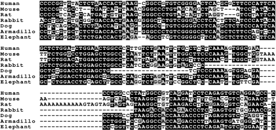
Figure 2: Multiple sequence alignment of length 180 from the HOXA region of seven mammalian genomes. Dashes indicate gaps; bases are colored according to their similarity across the species.

Phylogenetics depends on having identified homologous characters between the set of taxa. For example, historically, these characters might be physical characteristics of the organisms (for example, binary characters might include the following: are they unicellular or multicellular, cold-blooded or hot-blooded, egg-laying or placental mammals). In the era of genomics, the characters are typically single nucleotides or amino acids that have been inferred to be homologous (e.g., the first amino acid in a certain gene that is shared in a slightly different form among many organisms). For example, see Figure 2, which shows a multiple sequence alignment. We will throughout make the typical assumption that characters evolve independently, so that each column in Figure 2 is an independent, identically distributed (i.i.d.) sample from the model of evolution. While both DNA and amino acid data are common, we will work only with DNA and thus use the alphabet $\Sigma=\{\texttt{A},\texttt{C},\texttt{G},\texttt{T}\}$.

We assume that evolution happens via a continuous-time Markov process on a phylogenetic tree (see [41] for general details about Markov chains). That is, along each edge $e$ there is a length $t_{e}$ and a rate matrix $Q_{e}$ giving the instantaneous rates for evolution along edge $e$. Then $M_{e}=e^{Q_{e}t_{e}}$ is the transition matrix giving the probabilities of substitutions along the edge. In order to work with unrooted trees, we will assume that the Markov process is reversible, that is, $\pi_{i}M_{e}(i,j)=\pi_{j}M_{e}(j,i)$, where $\pi$ is the stationary distribution of $M_{e}$. In order for $e^{Q_{e}t_{e}}$ to be stochastic, we must have $Q(i,i)\leq 0$, $Q(i,j)\geq 0$ for $i\neq j$, and $\sum_{j}Q(i,j)=0$ for all $i$. Notice that since $\det(e^{Q})=e^{\mathrm{tr}(Q)}$, we can recover the branch length from the transition matrix $M_{e}$ as

$$t_{e}=\frac{1}{\mathrm{tr}Q_{e}}\log\det(M_{e}).$$ (1)

Example 2.2.

Let $Q_{e}=\begin{pmatrix}-1&\frac{1}{3}&\frac{1}{3}&\frac{1}{3}\\ \frac{1}{3}&-1&\frac{1}{3}&\frac{1}{3}\\ \frac{1}{3}&\frac{1}{3}&-1&\frac{1}{3}\\ \frac{1}{3}&\frac{1}{3}&\frac{1}{3}&-1\end{pmatrix}$ be the rate matrix for edge $e$, where the rows and columns are labeled by $\Sigma=\{\texttt{A},\texttt{C},\texttt{G},\texttt{T}\}$. Then

$$M_{e}=e^{Q_{e}t_{e}}=\frac{1}{4}\begin{pmatrix}1+3e^{-\frac{4}{3}t_{e}}&1-e^{-\frac{4}{3}t_{e}}&1-e^{-\frac{4}{3}t_{e}}&1-e^{-\frac{4}{3}t_{e}}\\ 1-e^{-\frac{4}{3}t_{e}}&1+3e^{-\frac{4}{3}t_{e}}&1-e^{-\frac{4}{3}t_{e}}&1-e^{-\frac{4}{3}t_{e}}\\ 1-e^{-\frac{4}{3}t_{e}}&1-e^{-\frac{4}{3}t_{e}}&1+3e^{-\frac{4}{3}t_{e}}&1-e^{-\frac{4}{3}t_{e}}\\ 1-e^{-\frac{4}{3}t_{e}}&1-e^{-\frac{4}{3}t_{e}}&1-e^{-\frac{4}{3}t_{e}}&1+3e^{-\frac{4}{3}t_{e}}\end{pmatrix}.$$

This form of rate matrix is known as the Jukes-Cantor model [33]. For example, the probability of changing from an A to a C along edge $e$ is given by $M_{e}(1,2)=\frac{1-e^{-\frac{4}{3}t_{e}}}{4}$.

Commonly used models that are more realistic than the Jukes-Cantor model include the Kimura 3-parameter model [35] where the rate matrices are of the form

$$\begin{pmatrix}\cdot&\gamma&\alpha&\beta\\ \gamma&\cdot&\beta&\alpha\\ \alpha&\beta&\cdot&\gamma\\ \beta&\alpha&\gamma&\cdot\end{pmatrix},$$

where $\cdot=-\gamma-\alpha-\beta$. See [42, Figure 4.7] for a description of many other possible models.

In order to obtain the joint distribution of characters at the leaves of the trees, we have to choose a root of the tree (arbitrarily, since the processes are time reversible), and run the Markov process down the edges of the tree, starting from a distribution of the characters at the root. The result is a joint probability distribution $p=(p_{\texttt{A}\dots\texttt{A}},\dots,p_{\texttt{T}\dots\texttt{T}})$, and the important point is that the coordinates of $p$ can be written as polynomials in the transition probabilities. That is, the model is specified parametrically by polynomials in the entries of $M_{e}$. We will forget about the specific form of the entries of $M_{e}=e^{Q_{e}t_{e}}$ and instead treat each entry of $M_{e}$ as an unknown. Thus for the Jukes-Cantor model, we have two unknowns per edge: $\alpha_{e}=\frac{1+3e^{-\frac{4}{3}t_{e}}}{4}$ and $\beta_{e}=\frac{1-e^{-\frac{4}{3}t_{e}}}{4}$. This makes the algebraic model more general than the statistical model (as it allows probabilities in the transition matrices to be negative or even complex). Although this allows algebraic tools to be used, we will see in Section 7 that it can be a disadvantage. Generally speaking, there are two types of phylogenetic models that have been thoroughly studied from the algebraic viewpoint: “group based” models such as the Jukes-Cantor and Kimura models, and variants of the general Markov model, in which no constraints are placed on the transition matrices.

In this paper, we define the phylogenetic invariants for a model of evolution and a tree to be the polynomials in the joint probabilities that vanish if the probabilities come from the model on the tree. For example, for a quartet tree (an unrooted binary tree with four leaves, see Figure 3) under the Jukes-Cantor model, $p_{\texttt{A}\texttt{A}\texttt{A}\texttt{A}}-p_{\texttt{C}\texttt{C}\texttt{C}\texttt{C}}=0$, due to the symmetry built into the model. However, this polynomial doesn’t differentiate between trees—it lies in the intersection of the ideals of the three quartet trees. Beware that there are two commonly used definitions of phylogenetic invariants. Originally, they were defined as polynomials that vanish on probability distributions arising from exactly one tree, so the above polynomial would be excluded. However, it is more algebraically convenient to take as invariants the full set of polynomials that vanish, as this forms an ideal. We spend the rest of this section deriving a particularly important polynomial.

A class of phylogenetic methods bypass working with the joint probability distribution and instead only estimate the distances between each pair of taxa. The goal then is to find a tree with branch lengths such that the distance along edges of the tree between pairs of leaves approximates the estimated pairwise distances. To use these distance methods, we first need a couple of definitions. We will concentrate in this paper on quartet trees, i.e., trees with four leaves. There are 3 different (unrooted, binary) trees on four leaves, we will write them $(01:23)$, $(02:13)$, and $(03:12)$, corresponding to which pairs of leaves are joined together.

Definition 2.3.

A dissimilarity map $d\in\mathbb{R}^{\binom{n}{2}}$ satisfies $d(i,j)=d(j,i)\geq 0$ and $d(i,i)=0$. We say that $d$ is a tree metric if there exists a phylogenetic tree $T$ with non-negative branch lengths $t_{e}$ such that for every pair $i,j$ of taxa, $d(i,j)$ is the sum of the branch lengths $t_{e}$ on the edges of $T$ connecting $i$ and $j$.

Proposition 2.4 (Four-point condition [10]).

A dissimilarity map $d$ is a tree metric if and only if for every $i,j,k,$ and $l$, the maximum of the three numbers

$$d_{ij}+d_{kl},\quad d_{ik}+d_{jl},\text{ and}\quad d_{il}+d_{jk}$$

is attained at least twice.

$$d_{01}+d_{23}\qquad\leq\quad\qquad d_{02}+d_{13}\quad\qquad=\qquad d_{03}+d_{12}$$

Figure 3: The four-point condition.

Example 2.5.

Let us restrict our attention to a tree with four leaves, $(ij:kl)$. In this case, the four-point condition becomes (see Figure 3)

$$d_{ij}+d_{kl}\leq d_{ik}+d_{jl}=d_{il}+d_{jk}.$$ (2)

The equality in the four-point condition can be translated into a quadratic polynomial in the probabilities, however, we first have to understand how to transform the joint probabilities into distances. Distances can be estimated from data in a variety of ways (there are different formulas for the maximum likelihood estimates of the distances under different models of evolution, see [23, Chapter 13]). The formula for the general Markov model is the logdet distance, which mimics what we saw above (1), in that a transition matrix is estimated and the distance is taken to be the log of the determinant of this matrix.

Here we will use a simpler formula for the distance, under the Jukes-Cantor model (Example 2.2). The maximum likelihood estimate of the distance between two sequences under the Jukes-Cantor model is given by $d_{ij}=-\frac{1}{4}\log\left(1-\frac{4m_{ij}}{3}\right)$ where $m_{ij}$ is the fraction of mismatches between the two sequences, e.g.,

$$m_{12}=\sum_{i,j,k,l\in\{\texttt{A},\texttt{C},\texttt{G},\texttt{T}\},i\neq j}p_{ijkl}$$

After plugging this distance into the four point condition, cancelling, and exponentiating, the equality in (2) becomes

$$\left(1-\frac{4}{3}m_{ik}\right)\left(1-\frac{4}{3}m_{jl}\right)-\left(1-\frac{4}{3}m_{il}\right)\left(1-\frac{4}{3}m_{jk}\right)=0.$$ (3)

We will call this polynomial the four-point invariant. This construction is originally due to Cavender and Felsenstein [14].

Example 2.5 shows one of the first constructions on a phylogenetic invariant, in the same year as the discovery by Lake of linear invariants [36]. There is a linear change of coordinates on the probability distribution $p$ under which $I(T)$ has a generating set of binomials. In particular, in these coordinates, a simple calculation shows that (3) becomes a binomial. Known as the Hadamard or Fourier transform [27, 52, 21, 50], this change of coordinates transforms the ideals of invariants for several models of evolution into toric ideals [49]. It should be emphasized, however, that this transform is only known to exist for group-based models.

The four-point invariant is a polynomial in the joint probabilities that vanishes on distributions arising from a certain quartet tree. Define the ideal $I_{\mathcal{M}}(T)$ of invariants for a model $\mathcal{M}$ of evolution on a tree $T$ to be the set of all polynomials that are identically zero on all probability distributions arising from the model $\mathcal{M}$ on $T$. We will write only $I(T)$ when $\mathcal{M}$ is clear from context.

3 How to use invariants

The basic idea of using phylogenetic invariants is as follows. A multiple sequence alignment DNA alignment of $n$ species gives rise to an empirical probability distribution $\hat{p}\in\mathbb{R}^{4^{n}}$. This occurs simply by counting columns of each possible type in the alignment, throwing out all columns that contain a gap (a “-” symbol). For example, Figure 2 has exactly one column that reads “CCCACCC” (the first) out of 107 gap-free columns total, so $\hat{p}_{\texttt{C}\texttt{C}\texttt{C}\texttt{A}\texttt{C}\texttt{C}\texttt{C}}=1/107$.

Then if $f$ is an invariant for tree $T$ under a certain model of evolution, we expect $f(\hat{p})\approx 0$ if (and generically only if) the alignment comes from the model on $T$. More precisely, where $\hat{p}_{N}$ is the empirical distribution after seeing $N$ observations from the model on $T$, then $\lim_{N\to\infty}E(f(\hat{p}_{N}))=0.$

We thus have a rough outline of how to use phylogenetic invariants to construct trees:

1. Choose a model $\mathcal{M}$ of evolution.

2. Choose a set of invariants $\mathbf{f}_{T}$ for model $\mathcal{M}$ for each tree $T$ with $n$ leaves.

3. Evaluate each set of invariants at $\hat{p}$.

4. Pick the tree $T$ such that $\mathbf{f}_{T}(\hat{p})$ is smallest (in some sense).

However, all of these steps contain difficulties: there are infinitely many polynomials to pick in exponentially many unknowns and exponentially many trees to compare. We will discuss step 2 in Section 4, step 3 in Section 6, and step 4 in Section 5. Selecting a model of evolution is difficult as well. There is, as always, a trade-off between biological realism (which could lead to hundreds of parameters per edge) and statistical usefulness of the model.

Since the rest of this paper will discuss difficulties with using invariants, we should stop and emphasize two especially promising features of invariants:

1. Invariants allow for arbitrary rate matrices.

One major challenge of phylogenetics is that evolution does not always happen at one rate. But common methods for constructing trees generally assume a single rate matrix $Q$ for all edges, leading to difficulties on data with heterogeneous rates. While methods have been developed to solve this problem (cf. [55, 25, 26]), it is a major focus of research.

In contrast, phylogenetic invariants allow for differing rate matrices within the chosen model on every edge (and in fact, even changing rate matrices along a single edge). The invariants for the Kimura 3-parameter model [35] have been shown to outperform neighbor-joining and maximum likelihood on quartet trees for heterogeneous simulated data [11]. To be fair, we should note that the invariants in this analysis were based on the correct model (i.e., the Kimura 3-parameter with heterogeneous rates, which the data was simulated from) while the maximum likelihood analysis used an incorrect model (with homogeneous rates) due to limitations in standard maximum likelihood packages.

2. Invariants perhaps can test individual features of trees.

Researchers are frequently interested in the validity of a single edge in the tree. For example, we might wonder if human or dog is a closer relative to the rabbit. This amounts to wondering about how much confidence there is in the edge between the human-rabbit-mouse-rat subtree and the dog subtree in Figure 1. There are methods, most notably the bootstrap [22] and Bayesian methods (cf. [32]), which provide answers to this question, but there are concerns about their interpretation [28, 16, 40, 1].

As for phylogenetic invariants, the generators of the ideal $I(T)$ are, in many cases, built from polynomials constructed from local features of the tree. Thus invariants seem to be well suited to test individual features of a tree. For example, suppose we have $n$ taxa. Consider a partition $\{A,B\}$ of the taxa into two sets. Construct the $|\Sigma|^{|A|}\times|\Sigma|^{|B|}$ matrix $\operatorname{Flat}_{A,B}(p)$ where the rows are indexed by assignments of $\Sigma$ to the taxa in $A$ and the columns by assignments of $\Sigma$ to the taxa in $B$. The entry of the matrix in a given row and column is the joint probability of seeing the corresponding assignments of $\Sigma$ to $A$ and $B$. The following theorem is [6, Theorem 4] and deals with the general Markov model, where there are no conditions on the form of the rate matrices.

Theorem 3.1 (Allman-Rhodes).

Let $\Sigma=\{0,1\}$ and let $T$ be a binary tree under the general Markov model. Then the $3\times 3$ minors of $\operatorname{Flat}_{A,B}(p)$ generate $I(T)$ for the general Markov model, where we let $A,B$ range over all partitions of $[n]$ that are induced by removing an edge of $T$.

While the polynomials in Theorem 3.1 do not generate the ideal for the DNA alphabet, versions of these polynomials do vanish for any Markov model on a tree. A similar result also holds for the Jukes-Cantor model in Fourier coordinates; the following is part of [50, Thm 2].

Theorem 3.2 (Sturmfels-Sullivant).

The ideal for the Jukes-Cantor DNA model is generated by polynomials of degree 1, 2, and 3 where the quadratic (resp. cubic) invariants are constructed in an explicit combinatorial manner from the edges (resp. vertices) of the tree.

Although there are many challenges to overcome, the fact that phylogenetic invariants are associated to specific features of a tree provides hope that they can lead to a new class of statistical tests for individual features on phylogenetic trees.

4 Choosing powerful invariants

There are, of course, infinitely many polynomials in each ideal $I(T)$, and it is not clear mathematically or statistically which should be used in the set $\mathbf{f}_{T}$ of invariants that we test. For example, we might hope to use a generating set, or a Gröbner basis, or a set that locally defines the variety, or a set that cuts out the variety over $\mathbb{R}$. We have no actual answers to this dilemma, but we provide a few illustrative examples and suggest possible criteria for an invariant to be powerful. We will deal with the Jukes-Cantor model on a tree with four leaves; the 33 generators for this ideal can be found on the “small trees” website www.shsu.edu/~ldg005/small-trees/ [13].

We believe that symmetry is an important factor in choosing powerful invariants. The trees with four leaves have a very large symmetry group: each tree can be written in the plane in eight different ways (for example, one tree can be written as (01 : 23), (10 : 23), …, (32 : 10)), and each of these induces a different order on the probability coordinates $p_{ijkl}$. This symmetry group ($\mathbb{Z}_{2}\times\mathbb{Z}_{2}\times\mathbb{Z}_{2}$) acts on the ideal $I(T)$ as well. In order that the results do not change under different orderings of the input, we should choose a set $\mathbf{f}_{T}$ of invariants that is closed (up to sign) under this action. After applying this action to the 33 generators, we get a set of 49 invariants. This symmetry will also play an important role in our metric learning algorithms in Section 5. See also [51] for a different perspective on symmetry in phylogenetics.

We begin by showing how different polynomials have drastically different behavior. Figure 4 shows the distribution of three of the invariants on data from simulations of alignments of length 1000 from the Jukes-Cantor model on $(01:23)$ for branch lengths ranging from $0.01$ to $0.75$ (similar to [30, 11, 20]). The histograms show the distributions for the simulated tree in white and the distributions for the other trees in gray and black.

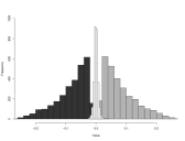
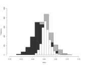
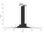
Four-point	Lake’s	Biased

Figure 4: Distributions of three invariants (the four-point invariant, Lake’s linear invariant, and a biased invariant) on simulated data. The white histogram corresponds to the correct tree, the black and gray are the other two trees. The invariants have quite different variances and performance.

The four-point invariant (left) distinguishes nicely between the three trees with the correct tree tightly distributed around zero. It is correct almost all of the time. Lake’s linear invariant (middle) also shows power to distinguish between all three trees, but distributions overlap much more—it is only correct about half of the time. The final polynomial seems to be biased towards selecting the wrong tree, even though it does not lie in $I(T)$ for either of the other two trees.

Figure 5 shows the performance of all the generators for this ideal on simulated data. The four-point invariant is the best, but the performance drops sharply with the other generators. Notably, the four-point invariant and several of the other powerful ones are unchanged (aside from sign) under the symmetries of the tree. While any invariant can be made symmetric by averaging, this behavior leads us to believe that invariants with a simple, symmetric form may be the best choice.

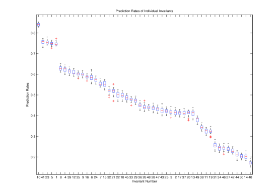
Figure 5: Prediction rate for the 49 Jukes-Cantor invariants on simulated data of length 100. The four-point invariant is by far the best, although four other invariants are quite good.

For more complex models, it becomes even more necessary to pick a good set of invariants since there are prohibitively many generators of the ideal. The paper [12] describes an algebraic method for picking a subset of invariants for the Kimura 3-parameter model, which has 11612 generators for the quartet tree (after augmenting by symmetry). Their method constructs a set of invariants which is a local complete intersection, and shows that this defines the variety on the biological relevant region. This reduces the list to 48 invariants which overall behave better than all 11612 invariants. However, of these 48, only 4 rank among the top 52 invariants in prediction rate (using simulations similar to those that produced Figure 5) and the remaining 44 invariants are mostly quite poor (42% average accuracy). This result, while of considerable theoretical interest, doesn’t seem to give an optimal set of invariants.

5 Comparing trees

Once we have chosen a set $\mathbf{f}_{T}$ of invariants for each tree $T$, we want to pick the tree such that $\mathbf{f}_{T}(\hat{p})$ is smallest (in some sense). The examples in Section 4 show why this is a non-trivial problem—different invariants have different power and different variance and thus should be weighted differently in choosing a norm on $\mathbf{f}_{T}$. In this section, we briefly describe an approach to normalizing the invariants to enable us to choose a tree. It is based on machine learning and was developed in [20]. It leads to large improvements over previous uses of invariants; however, it is computationally expensive and dependant on the training data. It can be thought of as finding the best single invariant which is a quadratic form in the starting set $\mathbf{f}_{T}$ of invariants.

There are also standard asymptotic statistical tools such as the delta method for normalizing invariants to have a common mean and variance. They have the disadvantage of depending on a linear approximation and asymptotic behavior, which might not be accurate for small datasets. Fortunately, the varieties for many phylogenetic models are smooth in the biologically significant region [12], so linear approximations may work well.

This problem is somewhat easier when we are choosing between different trees with the same (unlabelled) topology, for example, the three quartet trees. In this case the different ideals $I(T)$ are the same under a permutation of the unknowns, and thus we are comparing the same sets of polynomials (as long as the chosen set $\mathbf{f}_{T}$ is closed under the symmetries of $T$). For this reason, we will concentrate on the case of quartet trees and write $T_{1}=(01:23)$, $T_{2}=(02:13)$, and $T_{3}=(03:12)$.

Let $\hat{p}(\theta)$ be an empirical probability distribution generated from a phylogenetic model on tree $T_{1}$ with parameters $\theta$. Choose $m$ invariants $\mathbf{f}_{i}$ ($i=1,2,3$) that are closed under the symmetries of $T_{1}$. We want a norm $\|\ \|_{\ast}$ such that

$$\|\mathbf{f}_{1}(\hat{p}(\theta)))\|_{\ast}<\min\left(\|\mathbf{f}_{2}(\hat{p}(\theta))\|_{\ast},\|\mathbf{f}_{3}(\hat{p}(\theta))\|_{\ast}\right)$$ (4)

is typically true, i.e., the true tree should have its associated invariants closer to zero than others on the relevant range of parameter space.

In order to scale and weigh the individual invariants, the algorithm seeks to find an optimal $\|\ \|_{\ast}$ within the class of Mahalanobis norms. Recall that given a positive (semi)definite matrix $A$, the Mahalanobis (semi)norm $\|\cdot\|_{A}$ is defined by

$$\|x\|_{A}=\sqrt{x^{t}Ax}.$$

Since $A$ is positive semidefinite, it can be written as $A=UDU^{t}$ where $U$ is orthogonal and $D$ is diagonal with non-negative entries. Thus the positive semidefinite square root $B=U\sqrt{D}U^{t}$ is unique. Now since $\|x\|_{A}^{2}=x^{t}Ax=(Bx)^{t}(Bx)=\|Bx\|^{2}$, learning such a metric is the same as finding a transformation of the space of invariants that replaces each point $x$ with $Bx$ under the Euclidean norm, i.e., a rotation and shrinking/stretching of the original $x$.

Now suppose that $\Theta$ is a finite set of parameters from which training data $\mathbf{f}_{1}(\hat{p}(\theta)),\mathbf{f}_{2}(\hat{p}(\theta)),\mathbf{f}_{3}(\hat{p}(\theta))$ is generated for $\theta\in\Theta$. As we saw above, each of the eight possible ways of writing each tree induces a permutation of the coordinates $p_{ijkl}$ and thus induces a signed permutation of the coordinates of each $\mathbf{f}_{i}(\hat{p}(\theta))$. Write these permutations in matrix form as $\pi_{1},\dots,\pi_{8}$. Then the positive semidefinite matrix $A$ must satisfy the symmetry constraints $\pi_{i}A=A\pi_{i}$ which are hyperplanes intersecting the semidefinite cone. This symmetry condition is crucial in reducing the computational cost. Given training data, the following optimization problem finds a good metric on the space of invariants.

$$\begin{array}[]{ll}\text{Minimize: }&\sum_{\theta\in\Theta}\xi(\theta)+\lambda\mathrm{tr}A\\ \text{Subject to: }&\|\mathbf{f}_{1}(\hat{p}(\theta))\|_{A}^{2}+\gamma\leq\|\mathbf{f}_{i}(\hat{p}(\theta))\|_{A}^{2}+\xi(\theta)\quad(\text{for }i=2,3),\\ &\pi_{i}A=A\pi_{i}\quad(\text{for }1\leq i\leq 8),\\ &\xi(\theta)\geq 0,\quad\text{and}\\ &A\succeq 0,\end{array}$$ (5)

where $A\succeq 0$ denotes that $A$ is a positive semidefinite matrix, so this is a semidefinite programming problem. There are several parameters involved in this algorithm: $\xi(\theta)$ for $\theta\in\Theta$ are slack-variables measuring the violation of (4), $\gamma$ is a margin parameter that lets us strengthen condition (4), and $\lambda$ is a regularization parameter to keep the trace $\mathrm{tr}A$ small while keeping $A$ as low rank as possible. It tries to find a positive semidefinite $A$ at a trade-off between the small violation of (4) and small trace $A$.

The metric learning problem (5) was inspired by some early results on metric learning algorithms [53, 47], which aim to find a Mahalanobis (semi)norm such that the mutual distances between similar examples are minimized while the distances across dissimilar examples or classes are kept large. If it becomes too computationally expensive, we can restrict $A$ to be diagonal, which reduces the problem to a linear program. See [20] for details and simulation results. The learned metrics significantly improve on any of the individual invariants as well as on unweighted norms. The semidefinite programming algorithm is computationally feasible for approximately 100 invariants, and the choice of powerful invariants is important.

6 Efficient computation

At first glance, the problem of using invariants seems intractable for large trees for the simple reason that the number of unknowns grows exponentially with the number of leaves. However, the problem is not as bad as it may seem. Phylogenetic analyses typically use DNA sequences at most thousands of bases long, which means that the empirical distribution $\hat{p}\in\mathbb{R}^{4^{n}}$ will be extremely sparse even with a relatively small number of taxa.

Also the data can be sparse, this will not help unless we can write down the invariants in sparse form. If the polynomials can be written down in an effective way, they can be evaluated quickly. The determinantal form of the invariants in Theorem 3.1 provide such a form; see [18] for an algorithm to construct phylogenetic trees in polynomial time using these invariants and numerical linear algebra. Also see [2] for invariants that are (in some sense) determinantal. It seems that determinantal conditions could be particularly useful, so we suggest Problem 8.5 to computational commutative algebraists (see also [19]).

Unfortunately, for group-based models the polynomials are only sparse when written in Fourier coordinates, and the Fourier transform takes a sparse distribution $p$ and produces a completely dense vector $q$. Many of the invariants are determinantal in Fourier coordinates, but since the matrices are dense, they are difficult to write down. Can these polynomials be evaluated efficiently?

7 Positivity

Recall that the four point condition (Proposition 2.4 and Figure 3) says that for a dissimilarity map $d$ arising from the quartet tree $(01:23)$,

$$d_{01}+d_{23}\leq d_{02}+d_{13}=d_{03}+d_{12}.$$ (6)

This is true since the right two sums traverse the inner edge of the tree twice (Figure 3). We saw in Example 2.5 that the equality in (6) translates to a quadratic invariant. However, notice that if the interior branch of the tree has negative length, the equality is still satisfied, but the inequality changes so that $d_{01}+d_{23}$ is now larger than the other two sums.

The widely used neighbor-joining algorithm [43], when restricted to four taxa, reduces to finding the smallest of the three sums in the four-point condition. That is, neighbor-joining on a quartet tree involves estimating the distances as in Section 2 and then returning the tree $(ij:kl)$ that minimizes $d_{ij}+d_{kl}$. If instead we used the quadratic invariant arising from the equality in the four point condition, we would have an invariant based method that simply returns the tree $(ij:kl)$ that minimizes $|d_{ik}+d_{jl}-d_{il}-d_{jk}|$. We saw in Section 4 that this invariant performs quite well compared to the other generators of the Jukes-Cantor model. However, it compares poorly to the neighbor-joining criterion in the following way.

Figure 6 shows the difference between these two selection criteria on a projection of the six dimensional space of dissimilarity maps $\mathbb{R}^{\binom{4}{2}}$ to two dimensions. The three black lines are the projections of distances arising from the three different trees. Moving out from the center along these lines corresponds to increasing the length of the inner edge in the tree.

Geometrically, neighbor-joining can be thought of as finding the closest tree metric (a point on a black half-ray) to a dissimilarity map. The four-point invariant can’t distinguish negative inner branch length (the dotted black line) and thus is much less robust than neighbor-joining. Notice that even when it picks the wrong tree, it can pick the wrong wrong tree—that is, the one least supported by the data. It is less robust than neighbor-joining in the “Felsenstein zone” [31], which corresponds to the region close to the center, where the inner edge is very short.

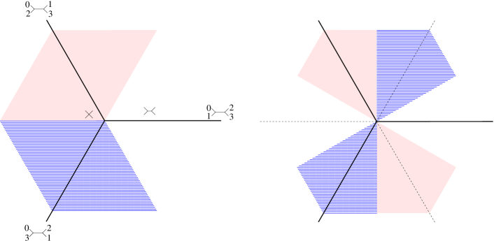
Figure 6: The selection criteria for neighbor-joining (left) and the four-point invariant (right) projected to two dimensions. The colored/shaded regions show which dissimilarity maps are matched to which trees by the two algorithms. The white/unshaded area corresponds to tree $(01:23)$, the red/solid area to tree $(02:13)$ and the blue/striped area to $(03:12)$.

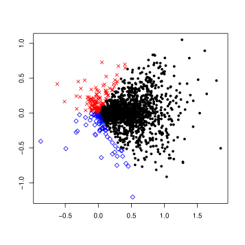
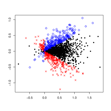
Neighbor joining	Four-point invariant

Figure 7: Illustration of Figure 6 on simulated data. Simulated alignments from tree $(01:23)$ of length 100 were created for randomly chosen branch lengths between $0.01$ and $0.75$. Distances were estimated using the Jukes-Cantor model and projected onto two dimensions in the same way as in Figure 6. Trees were built from the distances using both neighbor-joining and the four-point invariant. Black circles correspond to distances assigned tree $(01:23)$, red x’s to tree $(02:13)$, and blue diamonds to tree $(03:12)$.

Simulations (see Figure 7) show that building trees by evaluating this quadratic invariant does not perform nearly as well as neighbor-joining. This is because many simulations with a short interior branch tend to return metrics that seem to come from trees with negative inner branch lengths.

This seems to be a large blow to the method of invariants: even the most powerful invariant on our list in Section 4 doesn’t behave as well as this simple condition. However, it can be easily seen that testing the inequality is equivalent to testing the signs of the invariant instead of the absolute value, which leads us to ask if invariants can provide a way to discover conditions similar to that used in neighbor-joining (see Problem 8.7). The original paper of Cavender-Felsenstein [14] also suggested using inequalities, although no one seems to have followed up on this idea.

8 Open problems

Question 8.1.

Can algebraic ideas be used to estimate branch lengths and other parameters in phylogenetic trees? See [48, 7] for algebraic techniques for estimating parameters in invariable-site phylogenetic models.

Question 8.2.

Investigate the behavior of individual invariants on data from trees with heterogeneous rates. Are the best invariants the same ones that are powerful for homogeneous rates?

Question 8.3.

Can asymptotic statistical methods be practically used to normalize invariants? Do they give any information about the power of individual invariants?

Question 8.4.

Do the metrics constructed by the machine learning algorithm in Section 5 shed any light on the criteria for invariants to be powerful?

Question 8.5.

Define the “determinantal closure” of an ideal $I$ and develop algorithms to calculate it. See also [19].

Question 8.6.

For group-based models, does Fourier analysis provide a method to efficiently evaluate polynomials in the Fourier coordinates without destroying the sparsity of the problem? Note that many of the invariants are determinental in Fourier coordinates.

Question 8.7.

Are there other phylogenetic invariants (say for quartet trees under the Jukes-Cantor model) “similar” to the four-point invariant? We suggest the following conditions:

1. Be fixed (up to sign) under the $\mathbb{Z}_{2}\times\mathbb{Z}_{2}\times\mathbb{Z}_{2}$ symmetries of the quartet tree.

2. Have the following sign condition: $\pm f(p)>0$ for all $p$ from $T_{2}$ and $T_{3}$ (with perhaps a different choice of sign for $T_{2}$ and $T_{3}$). See for example, the symmetries of the left subfigure in Figure 4.

Beware that results such as [8] on the uniqueness of the neighbor-joining criterion place some constraints on whether we can hope to find invariants mimicking this behavior.

References

- [1] M. Alfaro, S. Zoller, and F. Lutzoni, Bayes or Bootstrap? A Simulation Study Comparing the Performance of Bayesian Markov Chain Monte Carlo Sampling and Bootstrapping in Assessing Phylogenetic Confidence, Molecular Biology and Evolution, 20 (2003), pp. 255–266.
- [2] E. S. Allman and J. A. Rhodes, Phylogenetic invariants for the general Markov model of sequence mutation, Mathematical Biosciences, 186 (2003), pp. 113–144.
- [3] , The identifiability of tree topology for phylogenetic models, including covarion and mixture models, J. Comput. Biol., 13 (2006), pp. 1101–1113 (electronic).
- [4] , Molecular phylogenetics from an algebraic viewpoint, Statistica Sinica, 17 (2007), pp. 1299–1316.
- [5] , Phylogenetic invariants, in Reconstructing evolution: new mathematical and computational advances, O. Gascuel and M. Steel, eds., Oxford University Press, 2007, ch. 4.
- [6] , Phylogenetic ideals and varieties for the general Markov model, Advances in Applied Mathematics, (2007, in press).
- [7] , Identifying evolutionary trees and substitution parameters for the general Markov model with invariable sites, Mathematical Biosciences, 211 (2008), pp. 18–33.
- [8] D. Bryant, On the Uniqueness of the Selection Criterion in Neighbor-Joining, Journal of Classification, 22 (2005), pp. 3–15.
- [9] W. Buczyńska and J. A. Wiśniewski, On geometry of binary symmetric models of phylogenetic trees, J. Eur. Math. Soc. (JEMS), 9 (2007), pp. 609–635.
- [10] P. Buneman, A note on the metric properties of trees, J. Combinatorial Theory Ser. B, 17 (1974), pp. 48–50.
- [11] M. Casanellas and J. Fernández-Sánchez, Performance of a new invariants method on homogeneous and nonhomogeneous quartet trees, Mol Biol Evol, 24 (2007), pp. 288–293.
- [12] , Geometry of the Kimura 3-parameter model, Adv Appl Math, to appear, 2008. arxiv.org/abs/math/0702834
- [13] M. Casanellas, L. D. Garcia, and S. Sullivant, Catalog of small trees, in Algebraic Statistics for Computational Biology, L. Pachter and B. Sturmfels, eds., Cambridge University Press, Cambridge, UK, 2005, ch. 15, pp. 291–304.
- [14] J. Cavender and J. Felsenstein, Invariants of phylogenies in a simple case with discrete states, Journal of Classification, 4 (1987), pp. 57–71.
- [15] D. Cox and J. Sidman, Secant varieties of toric varieties, J. Pure Appl. Algebra, 209 (2007), pp. 651–669.
- [16] B. Efron, E. Halloran, and S. Holmes, Bootstrap confidence levels for phylogenetic trees, Proceedings of the National Academy of Sciences, 93 (1996), pp. 13429–13429.
- [17] ENCODE Project Consortium, The ENCODE (ENCyclopedia Of DNA Elements) Project, Science, 306 (2004), pp. 636–40.
- [18] N. Eriksson, Tree construction using singular value decomposition, in Algebraic Statistics for Computational Biology, L. Pachter and B. Sturmfels, eds., Cambridge University Press, Cambridge, UK, 2005, ch. 19, pp. 347–358.
- [19] N. Eriksson, K. Ranestad, B. Sturmfels, and S. Sullivant, Phylogenetic algebraic geometry, in Projective varieties with unexpected properties, C. Ciliberto, A. Geramita, B. Harbourne, R.-M. Roig, and K. Ranestad, eds., Walter de Gruyter GmbH & Co. KG, Berlin, 2005, pp. 237–255.
- [20] N. Eriksson and Y. Yao, Metric learning for phylogenetic invariants, 2007. arXiv.org/abs/q-bio/0703034v1
- [21] S. Evans and T. Speed, Invariants of some probability models used in phylogenetic inference, The Annals of Statistics, 21 (1993), pp. 355–377.
- [22] J. Felsenstein, Confidence Limits on Phylogenies: An Approach Using the Bootstrap, Evolution, 39 (1985), pp. 783–791.
- [23] , Inferring Phylogenies, Sinauer Associates, Sunderland, MA, 2003.
- [24] , PHYLIP (phylogeny inference package) version 3.6. Available at http://evolution.genetics.washington.edu/phylip.html, 2005.
- [25] N. Galtier and M. Gouy, Inferring pattern and process: maximum-likelihood implementation of a nonhomogeneous model of DNA sequence evolution for phylogenetic analysis, Mol. Biol. Evol, 15 (1998), pp. 871–879.
- [26] O. Gascuel and S. Guindon, Modelling the variability of evolutionary processes, in Reconstructing evolution: new mathematical and computational advances, O. Gascuel and M. Steel, eds., Oxford University Press, 2007, ch. 3.
- [27] M. Hendy and D. Penny, A framework for the quantitative study of evolutionary trees, Systematic Zoology, 38 (1989).
- [28] D. Hillis and J. Bull, An Empirical Test of Bootstrapping as a Method for Assessing Confidence in Phylogenetic Analysis, Systematic Biology, 42 (1993), pp. 182–192.
- [29] R. Holmquist, M. Miyamoto, and M. Goodman, Analysis of higher-primate phylogeny from transversion differences in nuclear and mitochondrial DNA by Lake’s methods of evolutionary parsimony and operator metrics, Mol Biol Evol, 5 (1988), pp. 217–236.
- [30] J. Huelsenbeck, Performance of phylogenetic methods in simulations, Sys Biol, 1 (1995), pp. 17–48.
- [31] J. Huelsenbeck and D. Hillis, Success of Phylogenetic Methods in the Four-Taxon Case, Systematic Biology, 42 (1993), pp. 247–264.
- [32] J. Huelsenbeck, F. Ronquist, R. Nielsen, and J. Bollback, Bayesian Inference of Phylogeny and Its Impact on Evolutionary Biology, Science, 294 (2001), p. 2310.
- [33] T. Jukes and C. Cantor, Evolution of protein molecules, in Mammalian Protein Metabolism, H. Munro, ed., New York Academic Press, 1969, pp. 21–32.
- [34] Y. R. Kim, O.-I. Kwon, S.-H. Paeng, and C.-J. Park, Phylogenetic tree constructing algorithms fit for grid computing with SVD, 2006. arxiv.org/abs/q-bio.QM/0611015
- [35] M. Kimura, Estimation of evolutionary sequences between homologous nucleotide sequences, Proceedings of the National Academy of Sciences, USA, 78 (1981), pp. 454–458.
- [36] J. Lake, A rate-independent technique for analysis of nucleaic acid sequences: evolutionary parsimony, Molecular Biology and Evolution, 4 (1987), pp. 167–191.
- [37] F. Matsen, Phylogenetic mixtures on a single tree can mimic a tree of another topology, Systematic Biology, 56 (2007), pp. 767–775.
- [38] W. C. Navidi, G. A. Churchill, and A. von Haeseler, Methods for inferring phylogenies from nucleic acid sequence data by using maximum likelihood and linear invariants, Mol Biol Evol, 8 (1991), pp. 128–143.
- [39] , Phylogenetic inference: linear invariants and maximum likelihood., Biometrics, 49 (1993), pp. 543–555.
- [40] M. Newton, Bootstrapping phytogenies: Large deviations and dispersion effects, Biometrika, 83 (1996), p. 315.
- [41] J. Norris, Markov Chains, Cambridge University Press, 1997.
- [42] L. Pachter and B. Sturmfels, eds., Algebraic Statistics for Computational Biology, Cambridge University Press, Cambridge, UK, 2005.
- [43] N. Saitou and M. Nei, The neighbor joining method: a new method for reconstructing phylogenetic trees, Molecular Biology and Evolution, 4 (1987), pp. 406–425.
- [44] D. Sankoff and M. Blanchette, Phylogenetic invariants for metazoan mitochondrial genome evolution, Genome Informatics, (1998), pp. 22–31.
- [45] D. Sankoff and M. Blanchette, Comparative genomics via phylogenetic invariants for Jukes-Cantor semigroups, in Stochastic models (Ottawa, ON, 1998), vol. 26 of Proceedings of the International Conference on Stochastic Models, American Mathematical Society, Providence, RI, 2000, pp. 399–418.
- [46] C. Semple and M. Steel, Phylogenetics, vol. 24 of Oxford Lecture Series in Mathematics and its Applications, Oxford University Press, Oxford, 2003.
- [47] S. Shalev-Shwartz, Y. Singer, and A. Y. Ng, Online learning of pseudo-metrics, in Proceedings of the Twenty-first International Conference on Machine Learning, 2004.
- [48] M. Steel, D. Huson, and P. Lockhart, Invariable sites models and their use in phylogeny reconstruction, Systematic Biology, 49 (2000), pp. 225–232.
- [49] B. Sturmfels, Gröbner Bases and Convex Polytopes, vol. 8 of University Lecture Series, American Mathematical Society, 1996.
- [50] B. Sturmfels and S. Sullivant, Toric ideals of phylogenetic invariants, J Comput Biol, 12 (2005), pp. 457–481.
- [51] J. G. Sumner, M. A. Charleston, L. S. Jermiin, and P. D. Jarvis, Markov invariants, plethysms, and phylogenetics, 2007. arxiv.org/abs/0711.3503v2
- [52] L. Székely, M. Steel, and P. Erdős, Fourier calculus on evolutionary trees, Advances in Applied Mathematics, 14 (1993), pp. 200–210.
- [53] E. Xing, A. Y. Ng, M. Jordan, and S. Russell, Distance metric learning, with application to clustering with side-information, in NIPS, 2003.
- [54] Z. Yang, PAML: A program package for phylogenetic analysis by maximum likelihood, CABIOS, 15 (1997), pp. 555–556.
- [55] Z. Yang and D. Roberts, On the use of nucleic acid sequences to infer early branchings in the tree of life, Mol. Biol. Evol, 12 (1995), pp. 451–458.