TCDMATH 07–12

Fluctuations around the Tachyon Vacuum
in Open String Field Theory

O-Kab Kwon,^∗   Bum-Hoon Lee,^†§   Chanyong Park,^§   and Sang-Jin Sin^‡

* School of Mathematics, Trinity College, Dublin, Ireland
†Department of Physics, Sogang University, 121-742, Seoul, Korea
§Center for Quantum Spacetime, Sogang University, 121-742, Seoul, Korea
‡Department of Physics, Hanyang University, 133-791, Seoul, Korea

Abstract

We consider quadratic fluctuations around the tachyon vacuum numerically in open string field theory. We work on a space ${\cal H}_{N}^{{\rm vac}}$ spanned by basis string states used in the Schnabl’s vacuum solution. We show that the truncated form of the Schnabl’s vacuum solution on ${\cal H}_{N}^{{\rm vac}}$ is well-behaved in numerical work. The orthogonal basis for the new BRST operator $\tilde{Q}$ on ${\cal H}_{N}^{{\rm vac}}$ and the quadratic forms of potentials for independent fields around the vacuum are obtained. Our numerical results support that the Schnabl’s vacuum solution represents the minimum energy solution for arbitrary fluctuations also in open string field theory.

1 Introduction

After Schnabl’s analytic proof for Sen’s first conjecture [1] in Witten’s cubic open string field theory (OSFT) [2], there has been remarkable progress in analytic understanding of OSFT [3]-[19]. In particular, Sen’s third conjecture was proved analytically using the exactness of identity string state [5]. Analytic solutions for marginal deformations, especially, rolling tachyon solution, were constructed [12] and extended to superstring field theory [13]. General formalism for the marginal deformations including the case of singular operator products was constructed [17]. See also ref. [14] for other approaches in marginal deformations. And off-shell Veneziano amplitude in OSFT was calculated by employing a definition of the open string propagator in the Schnabl’s gauge [7, 19].

In this paper, we consider quadratic fluctuations written as $\tilde{Q}$-term in the action of OSFT numerically, construct an orthogonal basis, and investigate the stability of Schnabl’s vacuum solution and the structure of tachyon vacuum. Here $\tilde{Q}$ is a new BRST operator defined at the tachyon vacuum, which is composed of the original BRST operator $Q_{B}$ and tachyon vacuum solution $\Psi$. In virtue of the exact expression of the vacuum string field given by Schnabl [1], we construct the $\tilde{Q}$-term for arbitrary fluctuations in a subspace spanned by wedge state with operator insertions.

Before Schnabl’s breakthrough [1], there were many trials to understand the properties of $\tilde{Q}$ without exact expression of the vacuum solution [22]-[27]. Most of works in this area were devoted to the proof of vanishing cohomology of $\tilde{Q}$  [24, 23, 25, 27, 11] regarding to Sen’s third conjecture [28, 29]. As one of recent main analytic progresses of OSFT, the vanishing cohomology of $\tilde{Q}$ was proved by showing that all $\tilde{Q}$-closed states are $\tilde{Q}$-exact. Therefore, all fluctuation fields around the vacuum are off-shell ones according to the proof. To study the stability of the Schnabl’s vacuum solution and the tachyon vacuum structure in terms of potentials for independent fields, we restrict our interest to the spacetime independent gauge fixed off-shell fluctuations in $\tilde{Q}$-term neglecting the cubic interactions for the fluctuations.

In order to describe the physics around the vacuum completely, we have to take into account the string fluctuations governed by the $\tilde{Q}$-term on the full Hilbert space of OSFT. However, in numerical work, we have to take a subspace of the full Hilbert space by an appropriate approximation such as the well-known level truncation approximation [30]-[33]. In this work, we consider a truncated subspace spanned by basis string states which are used in Schnabl’s vacuum solution. Since the every basis state satisfies the Schnabl’s gauge condition, all fluctuations on the basis satisfy the Schnabl’s gauge condition. The vacuum solution is expressed by an infinite series in terms of wedge states with operator insertions. In construction of our truncated subspace, ${\cal H}_{N}^{{\rm vac}}$, we truncate the basis states up to wedge state $|N+2\rangle$ with operator insertions.

In section 2, we introduce a truncated Schnabl’s solution on ${\cal H}_{N}^{{\rm vac}}$ to use the Schnabl’s solution in numerical work. In $N\to\infty$ limit, the truncated Schnabl’s solution becomes the exact one. We examine the convergence and accuracy of the truncated Schnabl’s solution in BPZ inner product by increasing $N$.

In section 3, we consider spacetime independent arbitrary quadratic fluctuations and obtain orthogonal basis of $\tilde{Q}$ using the symmetric property of $\tilde{Q}$ on ${\cal H}_{N}^{{\rm vac}}$. We investigate the numerical properties of $\tilde{Q}$ for various situations, discuss the stability of Schnabl’s vacuum solution, and find quadratic forms of potential for independent fields around the tachyon vacuum. We conclude in section 4.

2 Truncated Schnabl’s Solution

We begin with a brief review of OSFT and an introduction of Schnabl’s analytic vacuum solution. The action of OSFT [2] has the form

$$S(\Phi)=-\frac{1}{g_{o}^{2}}\left[\frac{1}{2}\left<\Phi,\,Q_{{\rm B}}\Phi\right>+\frac{1}{3}\left<\Phi,\,\Phi*\Phi\right>\right],$$ (1)

where $g_{o}$ is the open string coupling constant, $Q_{{\rm B}}$ is the BRST operator, ‘$*$’ denotes Witten’s star product, and $\langle\cdot,\cdot\rangle$ is the BPZ inner product. In this definition of BPZ inner product, we omit the spacetime volume factor. The action (1) is invariant under the gauge transformation $\delta\Phi=Q_{{\rm B}}\Lambda+\Phi*\Lambda-\Lambda*\Phi$ for any Grassmann-even ghost number zero state $\Lambda$ and satisfies the classical field equation,

$$Q_{{\rm B}}\Phi+\Phi*\Phi=0.$$ (2)

Schnabl’s analytic vacuum solution of the Eq. (2) was represented as [1]

$$\Psi\equiv\lim_{N\to\infty}\left[\sum^{N}_{n=0}\psi_{n}^{{}^{\prime}}-\psi_{N}\right],$$ (3)

where $\psi_{n}$ and $\psi_{n}^{{}^{\prime}}\equiv\frac{\partial\psi_{n}}{\partial n}$ are the wedge state $|n+2\rangle$ [20, 21] with operator insertions, given by

$$\psi_{0}=\frac{2}{\pi}c_{1}|0\rangle,$$

$$\psi_{n}=\frac{2}{\pi}c_{1}|0\rangle*|n\rangle*B_{1}^{L}c_{1}|0\rangle,\qquad(n\geq 1)$$

$$\psi_{0}^{{}^{\prime}}=K_{1}^{L}c_{1}|0\rangle+B_{1}^{L}c_{0}c_{1}|0\rangle,$$

$$\psi_{n}^{{}^{\prime}}=c_{1}|0\rangle*K_{1}^{L}|n\rangle*B_{1}^{L}c_{1}|0\rangle,\qquad(n\geq 1).$$ (4)

Here we use the following operator representations on upper half plane(UHP),

$$B_{1}^{L}=\int_{C_{L}}\frac{d\xi}{2\pi i}(1+\xi^{2})b(\xi),$$

$$K_{1}^{L}=\int_{C_{L}}\frac{d\xi}{2\pi i}(1+\xi^{2})T(\xi),$$ (5)

where $b(\xi)$ is the $b$ ghost and the contour $C_{L}$ runs counterclockwise along the unit circle with ${\rm Re}\,z<0$. In obtaining the solution $\Psi$, Schnabl used clever coordinate $z=\tan^{-1}\xi$ and gauge choice

$${\cal B}_{0}\Psi=0,$$ (6)

where ${\cal B}_{0}=\oint\frac{d\xi}{2\pi i}(1+\xi^{2})\tan^{-1}\xi\,b(\xi)$.

We can describe the physics around the tachyon vacuum $\Psi$ by shifting the string field $\Phi=\Psi+\tilde{\Psi}$. Then the action in terms of string field $\tilde{\Psi}$ is given by

$$\tilde{S}(\tilde{\Psi})\equiv S(\Psi+\tilde{\Psi})-S(\Psi)=-\frac{1}{2}\langle\tilde{\Psi},\,\tilde{Q}\tilde{\Psi}\rangle-\frac{1}{3}\langle\tilde{\Psi},\,\tilde{\Psi}*\tilde{\Psi}\rangle,$$ (7)

where we set $g_{o}=1$ for simplicity. The new BRST operator $\tilde{Q}$ acts on a string field $\phi$ of ghost number $n$ through

$$\tilde{Q}\phi=Q_{{\rm B}}\phi+\Psi*\phi-(-1)^{n}\phi*\Psi.$$ (8)

It is straightforward to check the nilpotent property of $\tilde{Q}$ using the properties of the star products and the equation of motion for $\Psi$, $Q_{{\rm B}}\Psi+\Psi*\Psi=0$. The new action for the string field $\tilde{\Psi}$ has the same form as the original action (1) when $Q_{{\rm B}}$ and $\Psi$ are replaced by $\tilde{Q}$ and $\tilde{\Psi}$ respectively. So we can easily find the form of the gauge transformation for the action, $\delta\tilde{\Psi}=\tilde{Q}\tilde{\Lambda}+\tilde{\Psi}*\tilde{\Lambda}-\tilde{\Lambda}*\tilde{\Psi}$, with any Grassmann-even ghost number zero state $\tilde{\Lambda}$.

Our purpose in this paper is to investigate the physical properties of the new action $\tilde{S}(\tilde{\Psi})$ around the tachyon vacuum neglecting the cubic term in Eq. (7) numerically. To accomplish this purpose, we have to use the Schnabl’s solution according to the definition of $\tilde{Q}$ in Eq. (8). Most difficulties in numerical computations by using Schnabl’s solution come from the infinite series expression of it given in Eq. (3). To use the Schnabl’s solution in numerical work we have to truncate the infinite series somehow. As a truncation approximation similar to the well-known level truncation approximation in open string field theory [30, 31, 32, 33], we consider the following wedge state truncation for the solution (3),

$$\Psi_{N}=\sum_{n=0}^{N}\psi_{n}^{{}^{\prime}}-\psi_{N},$$ (9)

where $N$ is a finite number. We include the string states up to wedge state $|N+2\rangle$ in the truncated Schnabl’s solution (9). In this representation, the Schnabl’s solution $\Psi$ corresponds to $\Psi_{\infty}$.

$N$	$0$	$2$	$4$	$6$	$8$	$10$
$f(N)$	$-0.11289$	$-0.73227$	$-0.89030$	$-0.94163$	$-0.96400$	$-0.97564$
$N$	$20$	$40$	$60$	$80$	$100$	$200$
$f(N)$	$-0.99319$	$-0.99820$	$-0.99919$	$-0.99954$	$-0.99970$	$-0.99992$

Table 1: Values of $f(N)$ for various truncation numbers.

To use the truncated Schnabl’s solution instead of the tachyon vacuum solution $\Psi$ given in Eq. (3) in numerical computations, we have to check the properties of $\Psi_{N}$ in BPZ inner products. We insert $\Phi=\Psi_{N}$ into the action (1), and increase $N$ to figure out the properties of $\Psi_{N}$ in BPZ inner products. We compare this result with the well-known explicit result by Schnabl [1]. It was proved that $\Psi$ in Eq. (3) reproduces the exact tension ($=1/2\pi^{2}$ in $\alpha^{\prime}=1$ unit) of D25-brane expected by Sen’s first conjecture, i.e.,

$$S(\Psi)=-\frac{1}{2}\left<\Psi,\,Q_{{\rm B}}\Psi\right>-\frac{1}{3}\left<\Psi,\,\Psi*\Psi\right>=\frac{1}{2\pi^{2}},$$ (10)

where

$$\langle\Psi,\,Q_{{\rm B}}\Psi\rangle=-\frac{3}{\pi^{2}},\quad\langle\Psi,\,\Psi*\Psi\rangle=\frac{3}{\pi^{2}}.$$ (11)

In Table 1, we give the values of the normalized tachyon potential [29], $f(N)$, defined as

$$f(N)\equiv-2\pi^{2}S(\Psi_{N})$$ (12)

for various truncation numbers. From this numerical result, we see that the quantities $f(N)$ converge to the exact value $f(\infty)=-1$ with high accuracy as we increase $N$.

Figure 1: Graph of $f(N)$. The points represent $f(6),\,f(8),\,\cdots f(50)$ from the left.

In the usual level truncation approximation in OSFT, the normalized tachyon potential approaches to $-1$ as $L\to\infty$ non-monotonically [34, 33]. But in this wedge state truncation, $f(N)$ is a monotonic function with respective to $N$. In Fig.1, we plot the behavior of $f(N)$. Therefore, we can safely replace the infinite series of Schnabl’s solution $\Psi$ with the truncated Schnabl’s solution $\Psi_{N}$ for sufficiently large number of $N$ in the numerical computations of the BPZ inner products which contain the Schnabl’s solution.

3 Quadratic Fluctuations around the Tachyon Vacuum

Small fluctuations of string field $\tilde{\Psi}$ around the tachyon vacuum are governed by quadratic term in the action (7),

$$\tilde{S}_{0}(\tilde{\Psi})=-\frac{1}{2}\langle\tilde{\Psi},\,\tilde{Q}\tilde{\Psi}\rangle.$$ (13)

This action is composed of innumerable fields which are related each other in general. In this section, we investigate the properties of the spacetime independent fluctuations of $\tilde{\Psi}$. To do this we calculate the quantity $\langle\tilde{\Psi},\,\tilde{Q}\tilde{\Psi}\rangle$ numerically. In this calculation, we restrict our interests to arbitrary gauge fixed fluctuations with ghost number 1 on the space spanned by wedge states with some operator insertions, $\psi_{m}^{{}^{\prime}}$, $(m=0,1,2,\cdots)$, used in the expression of Schnabl’s solution (3). We construct the orthogonal basis of $\tilde{Q}$, which allows to define independent fields and obtain the quadratic potentials of the fields.

3.1 Orthogonal Basis of $\tilde{\Psi}$

In principle we have to consider the fluctuation field $\tilde{\Psi}$ on the full Hilbert space around the tachyon vacuum to study the physical properties of $\tilde{\Psi}$ given in the action (13). However, the Hilbert space around the vacuum is not well-known up to now. In our numerical work we restrict our interests to the fluctuation field $\tilde{\Psi}$ on the subspace spanned by basis states,

$${\cal H}^{{\rm vac}}_{N}\equiv{\rm span}\{\psi_{n}^{{}^{\prime}},\,0\leq n\leq N\}$$ (14)

with large but finite number of $N$.

Actually we can express the ordinary piece $\sum_{n=0}^{\infty}\psi_{n}^{{}^{\prime}}$ on the subspace ${\cal H}_{\infty}^{{\rm vac}}$ without the phantom piece $-\psi_{\infty}$ in Schnabl’s solution (3). The ordinary piece alone contributes to the vacuum energy about $50\%$ and the remaining contributions come from the interactions between the ordinary piece and phantom one and the phantom piece alone. So, the contribution of the phantom piece to the vacuum energy is nontrivial [1, 3]. If we parametrize the phantom piece like as $\alpha\psi_{\infty}$, we can easily see that the vacuum energy has the minimum value for the case $\alpha=-1$ which is the exact coefficient of $\psi_{\infty}$ in the phantom piece. Thus the energy contributions of the fluctuations along the direction of the phantom piece is positive always. However, the fluctuations which are expressed by the basis on ${\cal H}_{\infty}^{{\rm vac}}$ and $\psi_{\infty}$ simultaneously have nontrivial difficulties in the investigation of energy contributions by using our method which will be explained later. In this reason, we restrict our interests in the fluctuations on ${\cal H}_{N}^{{\rm vac}}$ only. We believe that this subspace is very important space in the tachyon condensation as we explained.

We express $\tilde{\Psi}$ on the truncated subspace spanned by $(N+1)$-basis states (14) as

$$\tilde{\Psi}_{N}=\sum_{n=0}^{N}c_{n}\psi_{n}^{{}^{\prime}},$$ (15)

where $c_{n}$ is an arbitrary small real number. Since each basis state satisfies

$${\cal B}_{0}\,\psi_{n}^{{}^{\prime}}=0,\quad(n\geq 0),$$ (16)

the fluctuation $\tilde{\Psi}_{N}$ in Eq. (15) satisfies the gauge choice

$${\cal B}_{0}\tilde{\Psi}_{N}=0.$$ (17)

In other words, we consider the gauge fixed fluctuations around the tachyon vacuum.

Inserting the Eq. (15) into the quantity $\langle\tilde{\Psi},\,\tilde{Q}\tilde{\Psi}\rangle$ in Eq. (13), we obtain

$$\langle\tilde{\Psi},\,\tilde{Q}\tilde{\Psi}\rangle_{N}=\sum_{m=0}^{N}\sum_{n=0}^{N}c_{m}c_{n}(\tilde{Q}_{N})_{mn},$$ (18)

where

$$(\tilde{Q}_{N})_{mn} \equiv \langle\psi_{m}^{{}^{\prime}},\,\tilde{Q}_{N}\psi_{n}^{{}^{\prime}}\rangle$$ (19)

$$= \langle\psi_{m}^{{}^{\prime}},\,Q_{{\rm B}}\psi_{n}^{{}^{\prime}}\rangle+\langle\psi_{m}^{{}^{\prime}},\,\Psi_{N}*\psi_{n}^{{}^{\prime}}\rangle+\langle\psi_{m}^{{}^{\prime}},\,\psi_{n}^{{}^{\prime}}*\Psi_{N}\rangle$$

$$= \frac{\partial}{\partial m}\frac{\partial}{\partial n}\,f(m,n)+2\sum_{k=0}^{N}\frac{\partial}{\partial m}\frac{\partial}{\partial k}\frac{\partial}{\partial n}\,h(m,k,n)-2\frac{\partial}{\partial m}\frac{\partial}{\partial n}\,h(m,N,n)$$

with $\Psi_{N}$ given in Eq. (9). Here $f(m,n)$ and $h(m,k,n)$ are the explicitly known formulae [1, 3],

$$f(m,n) \equiv \langle\psi_{n},Q_{{\rm B}}\psi_{m}\rangle$$ (20)

$$= \frac{1}{\pi^{2}}\,\left(1+\cos\frac{(m-n)\pi}{m+n+2}\right)\left(-1+\frac{m+n+2}{\pi}\sin\frac{2\,\pi}{m+n+2}\right)$$

$${}+2\sin^{2}\frac{\pi}{m+n+2}\left[\,-\frac{m+n+1}{\pi^{2}}+\frac{mn}{\pi^{2}}\cos\frac{(m-n)\pi}{m+n+2}\right.$$

$$\hskip 108.12054pt\left.+\frac{(m+n+2)(m-n)}{2\,\pi^{3}}\sin\frac{\pi\,(m-n)}{m+n+2}\,\right]\,,$$

$$h(m,k,n) \equiv \langle\psi_{n},\psi_{m}*\psi_{k}\rangle$$ (21)

$$= \frac{1}{2}\left(\frac{2}{\pi}\right)^{7}(m+n+k+3)^{2}\sin^{2}\left(\frac{\pi}{m+n+k+3}\right)$$

$$\times\sin\left(\frac{(n+1)\pi}{m+n+k+3}\right)\sin\left(\frac{(m+1)\pi}{m+n+k+3}\right)\sin\left(\frac{(k+1)\pi}{m+n+k+3}\right).$$

In the last step of Eq.(19) we used the symmetries among indices $m$, $k$, and $n$ in $h(m,k,n)$. which come from the twist symmetry of OSFT. Using the properties of the BPZ inner product and BRST operator $Q_{B}$, we can see that there is a symmetry between $m$ and $n$ in $f(m,n)$ also. So $(\tilde{Q}_{N})_{nm}$ is a matrix element of the real symmetric $(N+1)\times(N+1)$ matrix $\tilde{Q}_{N}$.

Since $\tilde{Q}_{N}$ is a finite dimensional real symmetric matrix, we can diagonalize $\tilde{Q}_{N}$ according to the following finite dimensional spectral theorem:

To every finite dimensional real symmetric matrix $A$ there exists a real orthogonal matrix $\tilde{U}$ such that $D=\tilde{U}A\tilde{U}^{T}$ is a diagonal matrix.

Here $\tilde{U}^{T}=\tilde{U}^{-1}$ is the transpose matrix of $\tilde{U}$. According to this theorem, we can diagonalize the matrix $\tilde{Q}_{N}$ by an orthogonal matrix $U$ as

$$\tilde{Q}_{N}=U^{T}\tilde{Q}_{N}^{(d)}U,$$ (22)

where $\tilde{Q}_{N}^{(d)}$ is a diagonalized matrix. Substituting the relation (22) into (18), we obtain

$$\langle\tilde{\Psi},\,\tilde{Q}\tilde{\Psi}\rangle_{N} = \sum_{m=0}^{N}\sum_{n=0}^{N}c_{m}(U^{T}\tilde{Q}_{N}^{(d)}U)_{mn}c_{n}$$ (23)

$$= \sum_{m=0}^{N}\bar{\lambda}_{m}\bar{c}_{m}^{2},$$

where the values $\bar{\lambda}_{m}$ are diagonal components of $\tilde{Q}_{N}^{(d)}$, i.e., eigenvalues of $\tilde{Q}_{N}$, and we define

$$\bar{c}_{m}=\sum_{n=0}^{N}U_{mn}c_{n}.$$ (24)

Since $c_{m}$ and all matrix elements $U_{mn}$ are real, the arbitrary coefficients $\bar{c}_{m}$ are also real. By comparing (18) with (23) and using the property of orthogonal matrix, $U^{T}=U^{-1}$, we obtain

$$\langle\bar{\psi}_{m},\,\tilde{Q}\bar{\psi}_{n}\rangle_{N}=\bar{\lambda}_{m}\delta_{mn},$$ (25)

where the orthogonal basis $\bar{\psi}_{m}$ is defined as

$$\bar{\psi}_{m}=\sum_{n=0}^{N}U_{mn}\psi_{n}^{{}^{\prime}}.$$ (26)

In the orthogonal basis (26), the truncated Schnabl’s solution (9) and the fluctuation string field (15) are written respectively as,

$$\Psi_{N}=\sum_{m=0}^{N}\sum_{n=0}^{N}U_{nm}\bar{\psi}_{n}-\psi_{N},\qquad\tilde{\Psi}=\sum_{m}^{N}\bar{c}_{m}\bar{\psi}_{m}.$$ (27)

3.2 Numerical results

To determine the diagonal components $\bar{\lambda}_{m}$ and the orthogonal matrix $U$ for a given truncation number $N$, we calculate the matrix elements of $\tilde{Q}_{N}$ given in Eq. (19) with the assistance of the MATHEMATICA program. During all processes of the numerical computations, we adjusted the number of significant digits by manipulating options of the program to increase numerical precisions. We calculate the matrix components of $\tilde{Q}_{N}$ up to $N=200$. In principle, we can obtain numerical results for the higher number of $N$ than $N=200$. As we will see in the numerical data, however, we can capture most of characteristic features of $\tilde{Q}_{N}$ by using the data up to $N=200$ sufficiently.

In our setup, we truncate the infinite dimensional matrix representation of $\tilde{Q}$ to a finite dimensional $(N+1)\times(N+1)$ matrix $\tilde{Q}_{N}$ with truncated Schnabl’s solution (9) for numerical work. Since the vacuum energy calculated from the truncated Schnabl’s solution $\Psi_{N}$ converges to the exact one by raising $N$ without any singularities [1, 3], the convergence of a certain quantity can be a criterion whether it is meaningful or not.

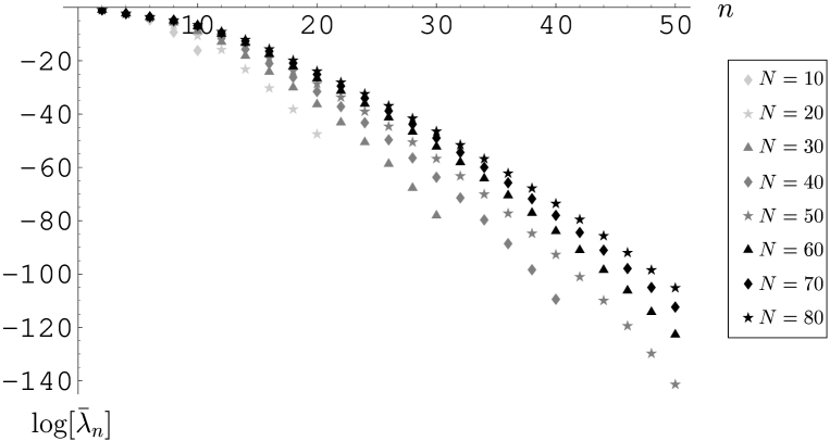
Figure 2: Graphs of $\log\bar{\lambda}_{n}$ for $n=2,\,4,\,6,\,\cdots 50$ on the truncated subspace ${\cal H}_{N}^{{\rm vac}}$, $(N=10,\,20,\,\cdots 80)$.

From the numerical results of $\tilde{Q}_{N}$, we determine the eigenvalues $\bar{\lambda}_{m}$ and the orthogonal matrix $U$ for a given $N$. In Table 2, we give eigenvalues of $\tilde{Q}_{N}$ for several truncation numbers of $N$. For positive eigenvalues, all eigenvalues, $\bar{\lambda}_{0}$, $\bar{\lambda}_{1}$, $\bar{\lambda}_{2}$, $\cdots$, seem to converge rapidly, i.e., $\bar{\lambda}_{m}$ for a given $m$ has a convergent series by raising $N$. For example, we explicitly show the convergent properties of $\bar{\lambda}_{m}$ for several largest eigenvalues in Table 3. We can also see the convergency of $\bar{\lambda}_{m}$ for a given $m$ graphically in Fig. 2.

Similarly to the eigenvalues of $\tilde{Q}_{N}$, the expansion coefficients of the orthogonal basis $\bar{\psi}_{m}$ with positive eigenvalues in Eq. (26) have convergent series as we increase $N$. For example, we give the lowest orthogonal state $\bar{\psi}_{0}$ which gives the largest eigenvalues $\bar{\lambda}_{0}$ for various truncation numbers of $N$,

$$N=0: \bar{\psi}_{0}=\psi_{0}^{{}^{\prime}},$$

$$N=1: \bar{\psi}_{0}=0.8123\psi_{0}^{{}^{\prime}}+0.5832\psi_{1}^{{}^{\prime}},$$

$$N=2: \bar{\psi}_{0}=0.9309\psi_{0}^{{}^{\prime}}+0.2798\psi_{1}^{{}^{\prime}}-0.2349\psi_{2}^{{}^{\prime}},$$

$$N=3: \bar{\psi}_{0}=0.8753\psi_{0}^{{}^{\prime}}+0.1228\psi_{1}^{{}^{\prime}}-0.3239\psi_{2}^{{}^{\prime}}-0.3374\psi_{3}^{{}^{\prime}},$$

$$N=4: \bar{\psi}_{0}=0.8521\psi_{0}^{{}^{\prime}}+0.1912\psi_{1}^{{}^{\prime}}-0.2686\psi_{2}^{{}^{\prime}}-0.3188\psi_{3}^{{}^{\prime}}-0.2521\psi_{4}^{{}^{\prime}}$$

$$N=5: \bar{\psi}_{0}=0.8384\psi_{0}^{{}^{\prime}}+0.2503\psi_{1}^{{}^{\prime}}-0.2196\psi_{2}^{{}^{\prime}}-0.2984\psi_{3}^{{}^{\prime}}-0.2514\psi_{4}^{{}^{\prime}}-0.1844\psi_{5}^{{}^{\prime}}.$$ (28)

For the higher numbers of $N$ than $N=5$, we found the similar convergent properties in the expression of $\bar{\psi}_{0}$. We also checked that the other orthogonal states, $\bar{\psi}_{n}$, $(n\geq 1)$, have the convergent series in their expansion coefficients by raising $N$. Using the expression of the orthogonal basis for a given $N$, we constructed the truncated Schnabl’s solution (27). We calculated the normalized tachyon potential $f(N)$ in Eq. (12) and found the same results in Table 1.

$N$	$\bar{\lambda}_{n}$
$0$	0.31496
$5$	0.41439,  0.27719,  0.072777  0.018645,  0.00087062,  0.000027315
$10$	0.40674,  0.29151,  0.085571,  0.054505,  0.0090014, 0.0014360,
	0.000089022,  5.9890$\times 10^{-6}$,  9.6021$\times 10^{-8}$,  1.1696$\times 10^{-9}$,  $-3.8026\times 10^{-10}$
	0.39960,  0.29724,  0.090905,  0.064312,  0.017602, 0.0046710,
$15$	0.00055827,  0.000073178,  4.3180$\times 10^{-6}$,  3.2883$\times 10^{-7}$, 3.4230$\times 10^{-9}$,
	6.7699$\times 10^{-11}$,  5.7708$\times 10^{-13}$,  7.2692$\times 10^{-15}$,  2.9800$\times 10^{-17}$,  $-2.9633\times 10^{-9}$
	0.39775,  0.29756,  0.096908,  0.064655,  0.022717, 0.0083524,
$20$	0.0013873,  0.00025064,  0.000024051,  2.8430$\times 10^{-6}$, 1.2781$\times 10^{-7}$,
	8.1196$\times 10^{-9}$,  8.3458$\times 10^{-11}$,  3.3754$\times 10^{-12}$,  7.0465$\times 10^{-14}$,  1.7739$\times 10^{-15}$,
	2.5832$\times 10^{-17}$,  3.3640$\times 10^{-19}$,  2.3055$\times 10^{-21}$,  8.8003$\times 10^{-24}$,  $-3.3857\times 10^{-8}$
	0.39739,  0.29702,  0.099841,  0.065190,  0.024882, 0.011712,
	0.0023989,  0.00053188,  0.000067479,  0.000010217, 7.6109$\times 10^{-7}$,
$25$	8.0343$\times 10^{-8}$,  1.5590$\times 10^{-9}$,  9.2397$\times 10^{-11}$,  2.8421$\times 10^{-12}$,  1.3550$\times 10^{-13}$,
	4.0610$\times 10^{-15}$,  1.3445$\times 10^{-16}$,  3.0310$\times 10^{-18}$,  6.6446$\times 10^{-20}$,  9.9971$\times 10^{-22}$,
	1.3095$\times 10^{-23}$,  1.0964$\times 10^{-25}$,  6.5095$\times 10^{-28}$,  1.6845$\times 10^{-30}$,  $-5.5178\times 10^{-9}$

Table 2: Eigenvalues of $\tilde{Q}_{N}$ for various $N$.

As we see in Table 2, the smallest eigenvalue for a given truncation number is negative. The first negative one appears from $N=9$ with magnitude $10^{-8}$. The second one appear from $N=98$. In our numerical range (up to $N=200$), there are only two negative eigenvalues. The negative eigenvalue $\bar{\lambda}_{-}$ decreases with oscillating behaviors for small $N$ (up to about $N=50$), and decreases very slowly for large $N$. $\bar{\lambda}_{-}$ almost stays around $10^{-8}$ in the range of our numerical experiments. The properties of the second one are similar to those of the first one.

	$N$=10	$N$=20	$N$=30	$N$=40	$N$=50
$\bar{\lambda}_{0}$	0.4067444	0.3977491	0.3973819	0.3974832	0.3975486
$\bar{\lambda}_{1}$	0.2915061	0.2975642	0.2965582	0.2960965	0.2959405
$\bar{\lambda}_{2}$	0.08557135	0.09690845	0.1009738	0.1013045	0.1010974
$\bar{\lambda}_{3}$	0.05450536	0.06465539	0.06625414	0.06825249	0.06937157
$\bar{\lambda}_{4}$	0.009001405	0.02271652	0.02550463	0.02572638	0.02654655
$\bar{\lambda}_{5}$	0.001435974	0.008352415	0.01446823	0.01789735	0.01898159
	$N$=60	$N$=70	$N$=80	$N$=90	$N$=100
$\bar{\lambda}_{0}$	0.3975807	0.3975964	0.3976044	0.3976086	0.3976110
$\bar{\lambda}_{1}$	0.2958885	0.2958715	0.2958665	0.2958658	0.2958664
$\bar{\lambda}_{2}$	0.1009304	0.1008443	0.1008076	0.1007954	0.1007940
$\bar{\lambda}_{3}$	0.06986604	0.07005325	0.07010889	0.07011381	0.07010217
$\bar{\lambda}_{4}$	0.02762730	0.02848060	0.02905543	0.02941796	0.02963724
$\bar{\lambda}_{5}$	0.01910793	0.01913351	0.01924661	0.01943154	0.01964400

Table 3: Several biggest eigenvalues, $\bar{\lambda}_{0},\,\bar{\lambda}_{1},\,\cdots\bar{\lambda}_{5}$, for $N=10,\,20,\,\cdots 100$.

The negative mode corresponds to the smallest eigenvalues for given $N$. Here we are dealing with approximation of infinite dimensional operator $\tilde{Q}$ with a sequence of finite dimensional one, and the approximation works in such a way that it matches approximately with the biggest eigenvalues and corresponding eigenvectors. To make sure this fact we investigate the validity of the negative eigenmode concretely. In order to figure out the negative mode for $\tilde{Q}$ in terms of the behaviors of eigenvalue, we need numerical data for very large number of $N$. However, it is a difficult problem because of computation time in the computer program. Instead of the eigenvalue, we investigated the behavior of coefficients in the negative eigenmode $\bar{\psi}_{-}=\sum_{n=0}^{N}U_{-n}\psi_{n}^{{}^{\prime}}$ given in Eq. (26). In the numerical work up to $N=200$, we found that 6 coefficients for lowest states, $U_{-i}$, ($i=0,\cdots,5$), converge. Several convergent coefficients are given in Table 4. For the coefficients for the higher states, we could not find convergent behaviors since they become irregular by raising $N$. We fitted the convergent coefficients and take the limit $N$ goes to infinity. We found the quantity $\langle\bar{\psi}_{-},\,\tilde{Q},\bar{\psi}_{-}\rangle$ is positive for the resulting coefficients in $N\to\infty$ limit. This result implies that the negativity of $\langle\bar{\psi}_{-},\,\tilde{Q}\,\bar{\psi}_{-}\rangle$ comes from the contribution of the higher states in $\bar{\psi}_{-}$, which have non-convergent coefficients. From this result, we can see that eigenvector $\bar{\psi}_{-}$ and its eigenvalue are not meaningful in our approximation.

Since we are considering spacetime independent fluctuations around the vacuum, the energy for the fluctuations is identified as

$$\Delta E=\frac{1}{2}\langle\tilde{\Psi},\,\tilde{Q}\tilde{\Psi}\rangle=\frac{1}{2}\sum_{m=0}^{N}\bar{\lambda}_{m}\bar{c}_{m}^{2}=-\tilde{S}_{0}.$$ (29)

Here $\Delta E$ corresponds to the energy difference from the vacuum energy. In our numerical work, all fluctuations which have convergent eigenvalues and eigenvectors with convergent coefficients have positive contributions to $\Delta E$. Therefore, our numerical result supports that the Schnabl’s vacuum solution is a minimum energy solution and stable for off-shell fluctuations also.

3.3 Potentials for various fields around the tachyon vacuum

In the previous subsection, we calculated the quantity $\langle\tilde{\Psi},\,\tilde{Q}\tilde{\Psi}\rangle$ with spacetime independent gauge fixed fluctuation $\tilde{\Psi}$ on ${\cal H}^{{\rm vac}}_{N}$. And we obtained the result (23) numerically. Inserting the Eq. (23) into the action (13) which is defined around the tachyon vacuum, we obtain

$$\tilde{S}_{0}(\bar{c}_{m})=-\frac{1}{2}\sum_{m=0}^{N}\bar{\lambda}_{m}\bar{c}_{m}^{2}.$$ (30)

	$N$=100	$N$=120	$N$=140	$N$=160
$U_{-0}$	$0.0021283$	$0.0023351$	$0.0024864$	$0.0025841$
$U_{-1}$	$-0.0085477$	$-0.0092470$	$-0.0097477$	$-0.010049$
$U_{-2}$	$0.047870$	$0.051303$	$0.053727$	$0.055103$
$U_{-3}$	$-0.18174$	$-0.19797$	$-0.19904$	$-0.20257$

Table 4: Coefficients for the several lowest states in the negative eigenmode

In this expression, $\tilde{S}_{0}$ is defined to be the action value divided by the spacetime volume factor according to the convention of BPZ inner product in this paper. Since we are considering spacetime independent fluctuations, $\tilde{S}_{0}$ can be written as the potential density around the tachyon vacuum,

$$V(\bar{\phi}_{m})=-\tilde{S}(\bar{\phi}_{m})=\frac{1}{2}\sum_{m=0}^{N}\bar{\lambda}_{m}\bar{\phi}_{m}^{2},$$ (31)

where we replace the arbitrary coefficients $\bar{c}_{m}$ with spacetime independent off-shell fields $\bar{\phi}_{m}$. For several largest eigenvalues, for instance, the potentials for independent fields are given by

$$V(\bar{\phi}_{m})=0.39761\,\bar{\phi}_{0}^{2}+0.29587\,\bar{\phi}_{1}^{2}+0.10082\,\bar{\phi}_{2}^{2}+0.070038\,\bar{\phi}_{3}^{2}+0.029882\,\bar{\phi}_{4}^{2}+\cdots,$$ (32)

where we used the data for $N=200$ case. The explicit numbers of $\bar{\lambda}_{m}$ for several truncation numbers $N$ were given in Table 2. The eigenvalues $\bar{\lambda}_{m}$ with fixed $N$ exponentially decrease with small oscillating behaviors as we increase $m$. For example, in the case $N=200$, $\bar{\lambda}_{m}$ has the following fitting curve,

$$\bar{\lambda}_{m}\sim e^{-0.6102\,m}.$$ (33)

4 Conclusion

We have investigated the behaviors of the quadratic fluctuations around the tachyon vacuum on the truncated subspace ${\cal H}_{N}^{{\rm vac}}$ numerically. We showed that the truncated form of Schnabl’s solution $\tilde{\Psi}_{N}$ is well-behaved on ${\cal H}_{N}^{{\rm vac}}$ and has nice convergence property by raising $N$ and high accuracy in BPZ inner product for large $N$. The physics around the vacuum is governed by $\tilde{S}_{0}(\tilde{\Psi})$ given in Eq. (13). In this paper we restricted our interest to the spacetime independent quadratic fluctuation $\tilde{\Psi}$. To calculate $\tilde{S}_{0}(\tilde{\Psi})$ on ${\cal H}_{N}^{{\rm vac}}$, we constructed the orthogonal string state $\bar{\psi}_{m}$, $(m=0,1,2,\cdots N)$, using the symmetric structure of $\tilde{Q}$ and obtained corresponding eigenvalues $\bar{\lambda}_{m}$.

The eigenvalues $\bar{\lambda}_{m}$ have nice convergence properties by raising $N$ also for small $m$. As we increase the truncation number $N$, the number of meaningful eigenvalues become large. In our numerical results, most of eigenvalues are positive but very small number of negative eigenvalues appear. The first one with magnitude $\sim 10^{-8}$ appears from $N=9$ and the magnitude of it very slowly grows according to the truncation number $N$. The second one appear from $N=98$ and has the same properties with the first one. As we argued in subsection 3.2, the negative modes are numerical artifacts of our setting. Thus all spacetime independent fluctuations around the vacuum have positive contribution to energy in the range of our numerical work. This result supports that the Schnabl’s vacuum solution is stable and represents minimum energy solution for off-shell fluctuations also.

Since we have taken into account the orthogonal basis states, the corresponding fields for the states have no interactions with other fields around the vacuum. Then the action $\tilde{S}_{0}(\tilde{\Psi})$ on ${\cal H}_{N}^{{\rm vac}}$ with spacetime independent fluctuation $\tilde{\Psi}$ corresponds to sum of quadratic forms of potentials with coefficients $\bar{\lambda}_{m}$ for the fields as given in Eq. (31). In canonical kinetic term with second order derivatives in field theory, there exist massive physical excitations for harmonic oscillator potential and $\bar{\lambda}_{m}$ corresponds to ${\rm mass}^{2}$ of the field $\bar{\phi}_{m}$. However, these phenomena do not happen since the absence of physical state including tachyon state at the vacuum was proved analytically [5]. Thus the shapes of quadratic potentials in our numerical results represent that the kinetic term at the tachyon vacuum has different form from the canonical second order differential operator and does not allow the physical excitations.

Extension of our work to the fluctuations with nonvanishing momentum will be helpful to figure out the role of kinetic term around the vacuum and to understand universal mechanism of vanishing of physical excitations by comparing with other theories, such as boundary string field theory, $p$-adic string theory, and DBI-type effective field theory, etc.

References

- [1] M. Schnabl, “Analytic solution for tachyon condensation in open string field theory,” Adv. Theor. Math. Phys. 10, 433 (2006) [arXiv:hep-th/0511286].
- [2] E. Witten, “Noncommutative Geometry And String Field Theory,” Nucl. Phys. B 268, 253 (1986).
- [3] Y. Okawa, “Comments On Schnabl’s Analytic Solution For Tachyon Condensation In Witten’s Open String Field Theory,” JHEP 0604, 055 (2006) [arXiv:hep-th/0603159]; E. Fuchs and M. Kroyter, “On the validity of the solution of string field theory,” JHEP 0605, 006 (2006) [arXiv:hep-th/0603195].
- [4] E. Fuchs and M. Kroyter, “Schnabl’s L(0) operator in the continuous basis,” JHEP 0610, 067 (2006) [arXiv:hep-th/0605254].
- [5] I. Ellwood and M. Schnabl, “Proof of vanishing cohomology at the tachyon vacuum,” JHEP 0702, 096 (2007) [arXiv:hep-th/0606142].
- [6] L. Rastelli and B. Zwiebach, “Solving open string field theory with special projectors,” arXiv:hep-th/0606131.
- [7] H. Fuji, S. Nakayama and H. Suzuki, “Open string amplitudes in various gauges,” JHEP 0701, 011 (2007) [arXiv:hep-th/0609047].
- [8] E. Fuchs and M. Kroyter, “Universal regularization for string field theory,” JHEP 0702, 038 (2007) [arXiv:hep-th/0610298].
- [9] Y. Okawa, L. Rastelli and B. Zwiebach, “Analytic solutions for tachyon condensation with general projectors,” arXiv:hep-th/0611110.
- [10] T. Erler, “Split string formalism and the closed string vacuum,” JHEP 0705, 083 (2007) [arXiv:hep-th/0611200]; T. Erler, “Split string formalism and the closed string vacuum. II,” JHEP 0705, 084 (2007) [arXiv:hep-th/0612050].
- [11] C. Imbimbo, “The spectrum of open string field theory at the stable tachyonic vacuum,” Nucl. Phys. B 770, 155 (2007) [arXiv:hep-th/0611343].
- [12] M. Schnabl, “Comments on marginal deformations in open string field theory,” arXiv:hep-th/0701248; M. Kiermaier, Y. Okawa, L. Rastelli and B. Zwiebach, “Analytic solutions for marginal deformations in open string field theory,” arXiv:hep-th/0701249.
- [13] T. Erler, “Marginal Solutions for the Superstring,” JHEP 0707, 050 (2007) [arXiv:0704.0930 [hep-th]]; Y. Okawa, “Analytic solutions for marginal deformations in open superstring field theory,” arXiv:0704.0936 [hep-th]; Y. Okawa, “Real analytic solutions for marginal deformations in open superstring field theory,” arXiv:0704.3612 [hep-th]; E. Fuchs and M. Kroyter, “Marginal deformation for the photon in superstring field theory,” arXiv:0706.0717 [hep-th].
- [14] E. Fuchs, M. Kroyter and R. Potting, “Marginal deformations in string field theory,” arXiv:0704.2222 [hep-th]; I. Kishimoto and Y. Michishita, “Comments on Solutions for Nonsingular Currents in Open String Field Theories,” arXiv:0706.0409 [hep-th].
- [15] I. Ellwood, “Rolling to the tachyon vacuum in string field theory,” arXiv:0705.0013 [hep-th]; N. Jokela, M. Jarvinen, E. Keski-Vakkuri and J. Majumder, “Disk Partition Function and Oscillatory Rolling Tachyons,” arXiv:0705.1916 [hep-th].
- [16] L. Bonora, C. Maccaferri, R. J. Scherer Santos and D. D. Tolla, “Ghost story. I. Wedge states in the oscillator formalism,” arXiv:0706.1025 [hep-th].
- [17] M. Kiermaier and Y. Okawa, “Exact marginality in open string field theory: a general framework,” arXiv:0707.4472 [hep-th]; M. Kiermaier and Y. Okawa, “General marginal deformations in open superstring field theory,” arXiv:0708.3394 [hep-th].
- [18] T. Erler, “Tachyon Vacuum in Cubic Superstring Field Theory,” arXiv:0707.4591 [hep-th].
- [19] L. Rastelli and B. Zwiebach, “The off-shell Veneziano amplitude in Schnabl gauge,” arXiv:0708.2591 [hep-th].
- [20] L. Rastelli and B. Zwiebach, “Tachyon potentials, star products and universality,” JHEP 0109, 038 (2001) [arXiv:hep-th/0006240]; M. Schnabl, “Wedge states in string field theory,” JHEP 0301, 004 (2003) [arXiv:hep-th/0201095].
- [21] L. Rastelli, A. Sen and B. Zwiebach, “Boundary CFT construction of D-branes in vacuum string field theory,” JHEP 0111, 045 (2001) [arXiv:hep-th/0105168].
- [22] L. Rastelli, A. Sen and B. Zwiebach, “String field theory around the tachyon vacuum,” Adv. Theor. Math. Phys. 5, 353 (2002) [arXiv:hep-th/0012251].
- [23] H. Hata and S. Teraguchi, “Test of the absence of kinetic terms around the tachyon vacuum in cubic string field theory,” JHEP 0105, 045 (2001) [arXiv:hep-th/0101162].
- [24] I. Ellwood and W. Taylor, “Open string field theory without open strings,” Phys. Lett. B 512, 181 (2001) [arXiv:hep-th/0103085].
- [25] I. Ellwood, B. Feng, Y. H. He and N. Moeller, “The identity string field and the tachyon vacuum,” JHEP 0107, 016 (2001) [arXiv:hep-th/0105024].
- [26] I. Kishimoto and T. Takahashi, “Open string field theory around universal solutions,” Prog. Theor. Phys. 108, 591 (2002) [arXiv:hep-th/0205275].
- [27] S. Giusto and C. Imbimbo, “Physical states at the tachyonic vacuum of open string field theory,” Nucl. Phys. B 677, 52 (2004) [arXiv:hep-th/0309164].
- [28] A. Sen, “Descent relations among bosonic D-branes,” Int. J. Mod. Phys. A 14, 4061 (1999) [arXiv:hep-th/9902105].
- [29] A. Sen, “Universality of the tachyon potential,” JHEP 9912, 027 (1999) [arXiv:hep-th/9911116].
- [30] V. A. Kostelecky and S. Samuel, “On A Nonperturbative Vacuum For The Open Bosonic String,” Nucl. Phys. B 336, 263 (1990).
- [31] A. Sen and B. Zwiebach, “Tachyon condensation in string field theory,” JHEP 0003, 002 (2000) [arXiv:hep-th/9912249].
- [32] N. Moeller and W. Taylor, “Level truncation and the tachyon in open bosonic string field theory,” Nucl. Phys. B 583, 105 (2000) [arXiv:hep-th/0002237].
- [33] D. Gaiotto and L. Rastelli, “Experimental string field theory,” JHEP 0308, 048 (2003) [arXiv:hep-th/0211012].
- [34] W. Taylor, “A perturbative analysis of tachyon condensation,” JHEP 0303, 029 (2003) [arXiv:hep-th/0208149].