Excitation of K-shell electrons by electron impact

Abstract

The universal scaling behavior for the electron-impact excitation cross sections of the $2s$ states of hydrogen- and helium-like multicharged ions is deduced. The study is performed within the framework of non-relativistic perturbation theory, taking into account the one-photon exchange diagrams. Special emphasis is laid on the near-threshold energy domain. The parametrical relationship between the cross sections for excitation of multicharged ions with different number of electrons is established.

1. Investigations of excitation processes of atomic ions by electron impact are of fundamental importance. During last decades, the problem has been intensively studied within the framework of different sophisticated approaches (see the works 1 ; 2 ; 3 ; 4 and references there). The deduction of the universal scaling behavior of the differential and total cross sections, which allows one to establish the generic features of the excitation processes, is of particular interest. In this Letter, we solve the problem within the framework of the consistent non-relativistic perturbation theory, taking into account the one-photon exchange diagrams. Special emphasis is laid on the near-threshold energy domain, because it requires the correct treatment of the electron-electron and electron-nucleus interactions.

2. Let us consider the inelastic scattering of an electron on hydrogen-like ion in the ground state, which results in excitation of a K-shell bound electron into the $2s$ state. We shall derive formulae for differential and total cross sections of the process in the leading order of non-relativistic perturbation theory with respect to the electron-electron interaction. The nucleus of an ion is treated as an external source of the Coulomb field. In a zeroth approximation, the Coulomb functions are employed as electron wave functions (Furry picture). The incident electron is characterized by the energy $E=\bm{p}^{2}/(2m)$ and the momentum $\bm{p}$ at infinitely large distances from the nucleus, while the scattered electron has the energy $E_{1}=\bm{p}_{1}^{2}/(2m)$ and the asymptotic momentum $\bm{p}_{1}$. The energy-conservation law reads $E=E_{1}+3I/4$, where $I=\eta^{2}/(2m)$ is the Coulomb potential for single ionization from the K shell, $\eta=m\alpha Z$ is the average momentum of the bound electron, $m$ is the electron mass, and $\alpha$ is the fine-structure constant ($\hbar=1$, $c=1$). Accordingly, the excitation process can occur, if $E\geqslant 3I/4$. The parameter $\alpha Z$ is supposed to be sufficiently small ($\alpha Z\ll 1$), although we assume that the nuclear charge $Z\gg 1$.

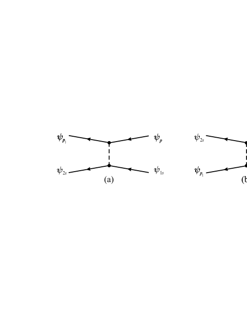
Figure 1: Feynman diagrams for excitation of the K-shell electron by electron impact. Solid lines denote electrons in the external Coulomb field of the nucleus, while dashed line denotes the electron-electron Coulomb interaction.

The process under consideration is described by the Feynman diagrams depicted in Fig. 1. In the initial and final continuum states, the single-electron wave functions are denoted by $\psi_{\bm{p}}$ and $\psi_{\bm{p}_{1}}$, respectively. Let us focus first on the asymptotic non-relativistic energies $E$ within the range $3I/4\ll E\ll m$. In this case, $E_{1}\sim E$ and the asymptotic momentum of the scattered electron is estimated as $p_{1}\sim p\gg\eta$. Accordingly, one needs to take into account only the Feynman diagram depicted in Fig. 1(a). The contribution of the exchange diagram turns out to be suppressed by the factor of about $(\eta/p)^{2}$ and, therefore, can be neglected. Then the amplitude of the process reads

$${\mathcal{A}}=\int\langle\psi_{\bm{p}_{1}}|\bm{f}_{1}\rangle\langle\bm{f}_{1}+\bm{f}|\psi_{\bm{p}}\rangle\frac{1}{f^{2}}\langle\psi_{2s}|\bm{f}_{2}\rangle\langle\bm{f}_{2}-\bm{f}|\psi_{1s}\rangle\frac{d\bm{f}}{(2\pi)^{3}}\frac{d\bm{f}_{1}}{(2\pi)^{3}}\frac{d\bm{f}_{2}}{(2\pi)^{3}}\,.$$ (1)

Note that the factor $4\pi\alpha$ originating from the photon propagator is shifted from the amplitude to the formula for the excitation cross section.

Since $p\sim p_{1}\gg\eta$, the wave functions of both the incident and scattered high-energy electrons can be approximated by the plane waves (Born approximation). Integration over the intermediate momenta in Eq. (1) leads to

$${\mathcal{A}} = N_{1s}\frac{1}{q^{2}}\Bigl{(}-\frac{\partial}{\partial\lambda}\Bigr{)}\langle\psi_{{2s}}|V_{i\lambda}|\bm{q}\rangle_{\left|\vphantom{\bigl{(}}\,\lambda=\eta\right.}\,,$$ (2)

$$\langle\bm{f}^{\prime}|V_{i\lambda}|\bm{f}\rangle = \frac{4\pi}{(\bm{f}^{\prime}-\bm{f})^{2}+\lambda^{2}}\,,$$ (3)

where $N^{2}_{1s}=\eta^{3}/\pi$ and $\bm{q}=\bm{p}-\bm{p}_{1}$ is the momentum transfer. After taking the derivative with respect to $\lambda$, one should set $\lambda=\eta$. Since the amplitude (2) is a function of the square of the momentum transfer $q^{2}$, it is convenient to introduce the dimensionless quantity $x=(q/\eta)^{2}$. Accordingly, the amplitude ${\mathcal{A}}$ can be cast into the form

$${\mathcal{A}} = N_{1s}N_{2s}\frac{1}{\eta^{5}}\,M\,,$$ (4)

$$M = \frac{2^{4}\pi}{(x+9/4)^{3}}\,,$$ (5)

where $N^{2}_{2s}=\eta_{2}^{3}/\pi$ and $\eta_{2}=\eta/2$.

The differential cross section for the $1s$-$2s$ excitation is related to the amplitude (4) via

$$d\sigma^{*}_{2s}=(4\pi\alpha)^{2}\frac{2\pi}{v}|{\cal A}|^{2}\frac{d^{3}\bm{p}_{1}}{(2\pi)^{3}}\,\delta(E-E_{1}-3I/4)\,.$$ (6)

Here $v=p/m$ is the absolute value of velocity of the incident electron. Equation (6) determines the energy and angular distributions of scattered electrons. The element of phase volume for electrons scattered into the solid angle $d\Omega_{1}$ can be written as

$$d^{3}\bm{p}_{1}=mp_{1}\,dE_{1}\,d\Omega_{1}=\pi\frac{m}{p}\,dE_{1}dq^{2}\,.$$ (7)

Integrating Eq. (6) over the energy $E_{1}$ yields

$$d\sigma^{*}_{2s}=\frac{\sigma_{0}}{Z^{4}}\frac{M^{2}}{2\pi^{2}\varepsilon}\,dx\,.$$ (8)

Here $\sigma_{0}=\pi a_{0}^{2}=87.974$ Mb, where $a_{0}=1/(m\alpha)$ is the Bohr radius. The dimensionless function $M$ is given by the expression (5). In Eq. (8), we have also introduced the dimensionless energy $\varepsilon=E/I$ of the incident electron. The energy-conservation law implies $\varepsilon=\varepsilon_{1}+3/4$, where $\varepsilon_{1}=E_{1}/I$ denotes the dimensionless energy of the scattered electron.

To obtain the total cross section for the excitation of a K-shell electron into the $2s$ state, the expression (8) should be integrated over the variable $x$ within the range from $x_{1}=(p-p_{1})^{2}/\eta^{2}$ to $x_{2}=(p+p_{1})^{2}/\eta^{2}$. This integration can be performed analytically 5 . The leading high-energy contribution appears, while extending the integration from $x_{1}=0$ to $x_{2}=\infty$. In this case, one obtains

$$\sigma^{*}_{2s} = \frac{\sigma_{0}}{Z^{4}}\,Q(\varepsilon)\,,$$ (9)

$$Q(\varepsilon) = \frac{2^{7}}{\varepsilon}\int_{0}^{\infty}\frac{dx}{(x+9/4)^{6}}=\frac{2^{17}}{3^{10}5\varepsilon}\,.$$ (10)

The quantity $Z^{4}\sigma^{*}_{2s}$ is a universal function of the dimensionless energy $\varepsilon$ of the incident electron. The universal scaling $Q(\varepsilon)$ does not account for the exchange effects and has a typical behavior for the excitation of states with the zeroth matrix element of the dipole transition 6 . Equation (10) holds true only within the asymptotic non-relativistic range $3/4\ll\varepsilon\ll 2(\alpha Z)^{-2}$.

Within the near-threshold domain, both the initial and final electron momenta $p$ and $p_{1}$ are of the order of a characteristic atomic momentum $\eta$. Correspondingly, the process occurs at atomic distances of the order of the K-shell radius. This implies that the Coulomb wave functions for both discrete and continuous spectra should be employed already in zeroth approximation. In this case, the direct and exchange Feynman diagrams depicted in Fig. 1 are expected to give comparable contributions to the excitation cross section.

Since the general method for evaluation of the Coulomb matrix elements has been already described in details in Ref. 7 , we present here the explicit expression for the amplitude $\mathcal{A}=\sum\limits_{\beta}\mathcal{A}_{\beta}$ without derivation. The individual contributions of both diagrams in Figs. 1(a) and (b) read

$$\mathcal{A}_{\mathrm{a}} = N_{1s}N_{2s}N_{p}N_{p_{1}}\dfrac{1}{\eta^{5}}\,M_{\mathrm{a}}\,\delta_{\tau_{1}^{\prime}\tau_{1}^{\vphantom{{}^{\prime}}}}\delta_{\tau_{2}^{\prime}\tau_{2}^{\vphantom{{}^{\prime}}}}\,,$$ (11)

$$\mathcal{A}_{\mathrm{b}} = N_{1s}N_{2s}N_{p}N_{p_{1}}\dfrac{1}{\eta^{5}}\,M_{\mathrm{b}}\,\delta_{\tau_{2}^{\prime}\tau_{1}^{\vphantom{{}^{\prime}}}}\delta_{\tau_{1}^{\prime}\tau_{2}^{\vphantom{{}^{\prime}}}}\,,$$ (12)

$$M_{\mathrm{a}} = \frac{8\pi}{9}\,\xi^{3}\frac{1}{2\pi i}\oint_{\gamma}\frac{dx}{x}\Bigl{(}\frac{-x}{1-x}\Bigr{)}^{i\xi}\biggl{\{}\xi\frac{\partial^{2}\Phi_{\mu}}{\partial\mu^{2}}-\frac{2}{3}\frac{\partial\Phi_{\mu}}{\partial\mu}\biggr{\}}_{\left|\vphantom{\bigl{(}}\,\mu=3\xi/2\right.}\,,$$ (13)

$$M_{\mathrm{b}} = \frac{2}{\pi}\,\xi^{4}\Gamma_{\zeta}\frac{\partial^{2}}{\partial\zeta\partial\lambda}\int_{0}^{\infty}dy\int d\bm{\nu}\,\Phi(\bm{y})\Phi_{1}(\bm{y}){}_{\left|{\lambda=\xi\hphantom{/2}}\atop{\zeta=\xi/2}\right.}\,,$$ (14)

$$\Phi_{\mu} = \frac{\left((\bm{n}_{1}\varkappa-\bm{n}(1-x))^{2}-(x+i\mu)^{2}\right)^{i\xi_{1}-1}}{\left((1-x)^{2}-(\varkappa+x+i\mu)^{2}\right)^{i\xi_{1}}}\,,$$ (15)

$$\Phi(\bm{y}) = \frac{\left((\bm{n}-\bm{y})^{2}+\zeta^{2}\right)^{i\xi-1}}{\left(y^{2}-(1+i\zeta)^{2}\right)^{i\xi}}\,,$$ (16)

$$\Phi_{1}(\bm{y}) = \frac{\left((\bm{n}_{1}\varkappa-\bm{y})^{2}+\lambda^{2}\right)^{i\xi_{1}-1}}{\left(y^{2}-(\varkappa+i\lambda)^{2}\right)^{i\xi_{1}}}\,,$$ (17)

$$\Gamma_{\zeta} = 1+\frac{\xi}{2}\frac{\partial}{\partial\zeta}\,,\quad\varkappa=\sqrt{1-3/(4\varepsilon)}\,,$$ (18)

$$\bm{n} = \frac{\bm{p}}{p}\,,\quad\bm{n}_{1}=\frac{\bm{p}_{1}}{p_{1}}\,,\quad\bm{\nu}=\frac{\bm{y}}{y}\,,$$ (19)

$$\xi = \frac{1}{\sqrt{\varepsilon}}\,,\quad\xi_{1}=\frac{1}{\sqrt{\varepsilon_{1}}}=\frac{1}{\sqrt{\varepsilon-3/4}}\,,$$ (20)

$$N^{2}_{p} = \frac{2\pi\xi}{1-e^{-2\pi\xi}}\,,\quad N^{2}_{p_{1}}=\frac{2\pi\xi_{1}}{1-e^{-2\pi\xi_{1}}}\,.$$ (21)

In Eq. (13), the integration contour $\gamma$ is a closed curve encircling counter-clockwise the points 0 and 1. After taking the derivatives in Eq. (13) with respect to the parameter $\mu$, one should set $\mu=3\xi/2$. In Eq. (14), after taking the derivatives over $\lambda$ and $\zeta$, the parameters should be set equal to $\lambda=\xi$ and $\zeta=\xi/2$, respectively. The quantities $\tau_{1,2}^{\vphantom{{}^{\prime}}}$ and $\tau_{1,2}^{\prime}$ denote the spin projections of the Pauli spinors in the initial and final states, respectively.

The formulae (11)–(21) define the amplitude $\mathcal{A}=\sum\limits_{\beta}\mathcal{A}_{\beta}$ of the electron-impact excitation, in which the initial and final electrons are characterized by definite polarizations. However, one is usually interested in the processes, in which the initial particles are not polarized, while polarizations of particles in the final state are not measured. Accordingly, the differential cross section (6) should be averaged over the polarizations of the initial electrons and summed over the polarizations of the final electrons. This can be achieved by means of the following substitution

$$|{\cal A}|^{2}\to\overline{\vphantom{{\cal A}^{2}}|{\cal A}|\,}\!{}^{2}=\frac{1}{4}\sum_{\tau_{1}^{\vphantom{{}^{\prime}}},\tau_{1}^{\prime}}\sum_{\tau_{2}^{\vphantom{{}^{\prime}}},\tau_{2}^{\prime}}|{\cal A}|^{2}\,,$$ (22)

where summations are performed over the electron polarizations in both the initial and final states. The angular distribution of the scattered electrons is given by

$$\frac{d\sigma^{*}_{2s}}{d\Omega_{1}} = \frac{\sigma_{0}}{Z^{4}}\,F(\varepsilon,\theta)\,,$$ (23)

$$F(\varepsilon,\theta) = \frac{2}{\pi}\frac{\xi^{2}\,T}{(1-e^{-2\pi\xi})(1-e^{-2\pi\xi_{1}})}\,,$$ (24)

$$T = \frac{1}{4}|M_{+}|^{2}+\frac{3}{4}|M_{-}|^{2}\,.$$ (25)

Here the dimensionless functions $M_{\pm}=M_{\mathrm{a}}\pm M_{\mathrm{b}}$, where particular contributions of the direct and exchange diagrams are given by Eqs. (13) and (14), respectively. Due to the azimuthal symmetry of the problem, the solid angle $d\Omega_{1}$ is just $d\Omega_{1}=2\pi\sin\theta d\theta$, where $\theta$ is the angle between the vectors $\bm{n}$ and $\bm{n}_{1}$.

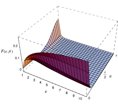
Figure 2: The universal function $F(\varepsilon,\theta)$ is calculated according to Eqs. (24) and (25) with respect to the dimensionless energy $\varepsilon$ of the incident electron and the scattering angle $\theta$.

The two-parameter function $F(\varepsilon,\theta)$, which is universal for the non-relativistic energies $\varepsilon$ of the incident electron within the range $3/4\leqslant\varepsilon\ll 2(\alpha Z)^{-2}$ and for any scattering angles $0\leqslant\theta\leqslant\pi$, is depicted in Fig. 2 within the near-threshold domain. In Figs. 3–7, we present also the energy behavior of the function $F(\varepsilon,\theta)$ for a few particular angles $\theta=0$, $\pi/4$, $\pi/2$, $3\pi/4$, and $\pi$, respectively. As it is seen, for energies $3/4\leqslant\varepsilon\lesssim 1$ the backward scattering is more preferable rather than the forward scattering. In this case, the correct account for both the direct and exchange diagrams appears to be extremely crucial. However, with increasing energy $\varepsilon$, the situation changes rapidly to the opposite: the forward scattering becomes much more pronounced, while the backward scattering turns out to be negligible. At high energies $\varepsilon\gg 1$, the dominant contribution arises from the direct diagram only.

Integrating Eq. (23) over the solid angle yields the total cross section

$$\sigma^{*}_{2s} = \frac{\sigma_{0}}{Z^{4}}Q(\varepsilon)\,,$$ (26)

$$Q(\varepsilon) = 2\pi\int_{0}^{\pi}\!F(\varepsilon,\theta)\sin\theta d\theta\,,$$ (27)

where $F(\varepsilon,\theta)$ is given by Eq. (24). The universal function $Q(\varepsilon)$, which describes the whole family of hydrogen-like targets with moderate nuclear charges $Z$, is depicted in Fig. 8. For comparison, we also draw there the high-energy scaling (10) obtained within the framework of the Born approximation. Although the latter is not applicable within the near-threshold energy domain, the plane-wave results appear to be in reasonable agreement with the exact predictions. For example, at the threshold energy $\varepsilon_{\mathrm{th}}=3/4$, Eq. (27) yields $Q(\varepsilon_{\mathrm{th}})=0.482$, while according to Eq. (10) one receives just $Q(\varepsilon_{\mathrm{th}})=2^{19}/(3^{11}5)=0.592$.

It should be noted that the behavior of the universal function $Q(\varepsilon)$ calculated according to Eq. (27) is relatively close to that presented in the work 4 . However, the numerical calculations performed in Ref. 4 for different hydrogen-like ions within the framework of sophisticated methods exhibit a slight dependence on the nuclear charge even for the moderate values of $Z$ .

Just above the threshold, the $1s$-$2s$ excitation cross section measured for the He⁺ ion was found to be $\sigma^{*}_{2s}/\sigma_{0}=0.0128$ 8 . Our prediction according to Eq. (26) is equal to $\sigma^{*}_{2s}/\sigma_{0}=0.03$. The significant deviation of these results seems to be caused by the correlation corrections due to two-photon exchange diagrams, which have been neglected in the present consideration.

3. Now we shall study the inelastic electron scattering on helium-like ion in the ground state followed by the excitation of a K-shell electron into the $2s$ state. To leading order of the non-relativistic perturbation theory with respect to the electron-electron interaction, one needs to consider only the Feynman diagrams with one-photon exchange. In this case, it is sufficient to take into account the interaction between two active electrons, which participate in the excitation process. The interaction with the second electron of target (spectator) is neglected, since it first contributes only in the next-to-leading order of the perturbation theory. Accordingly, the problem can be reduced to that studied in the previous paragraph.

First, we shall obtain the cross section for impact excitation of helium-like ion into the $1s2s$ configuration, when the energy terms with different spin multiplicities cannot be resolved experimentally. In this case, taking into account the number of target electrons, the cross sections for helium- and hydrogen-like ions are related as follows

$$d\sigma^{*}(\mathrm{He})=2\,d\sigma^{*}_{2s}\,,$$ (28)

where $d\sigma^{*}_{2s}$ is given by Eqs. (23)–(25). Integrating Eq. (28) over the solid angle $d\Omega_{1}$ yields a similar relation for the total cross sections.

Another situation occurs, if one can experimentally distinguish the excitations into the singlet $2^{1}S$ and the triplet $2^{3}S$ states of helium-like ion. The corresponding cross sections, $d\sigma_{\mathrm{s}}^{*}(\mathrm{He})$ and $d\sigma_{\mathrm{t}}^{*}(\mathrm{He})$, are given by the formulae similar to Eqs. (23) and (24), where the dimensionless function $T$ is given by

$$T=\begin{cases}\dfrac{2}{4}|2M_{\mathrm{a}}-M_{\mathrm{b}}|^{2},&\text{singlet $2^{1}S$ state}\,;\\ 2\dfrac{3}{4}|M_{\mathrm{b}}|^{2},&\text{triplet $2^{3}S$ state}\,.\end{cases}$$ (29)

Here the factor 2 accounts for the number of electrons in a helium-like ion. The factors $1/4$ and $3/4$ are the statistical weights for the singlet and triplet states, respectively. The dimensionless functions $M_{\mathrm{a}}$ and $M_{\mathrm{b}}$ are given by Eqs. (13) and (14). As it is seen, the excitation of the triplet $2^{3}S$ state occurs only due to the exchange interaction. In Figs. 9 and 10, we present the universal functions $F(\varepsilon,\theta)$ describing the energy and angular behavior of the differential cross sections for excitation of helium-like ion into the $2^{1}S$ and the $2^{3}S$ states, respectively. In Figs. 11 and 12, the same functions $F(\varepsilon,\theta)$ are given with respect to the dimensionless energy for the forward ($\theta=0$) and backward ($\theta=\pi$) scattering, respectively. Integrating the functions $F(\varepsilon,\theta)$ over the solid angle yields the universal functions $Q(\varepsilon)$, which define the energy dependence of the total cross sections $\sigma_{\mathrm{s,t}}^{*}(\mathrm{He})$ (see Fig. 13). The latter obey universal scalings similar to that given by Eq. (26).

The averaged cross section for excitation of helium-like ion into the $1s2s$ configuration can be written as

$$d\sigma^{*}(\mathrm{He})=d\sigma_{\mathrm{s}}^{*}(\mathrm{He})+d\sigma_{\mathrm{t}}^{*}(\mathrm{He})\,,$$ (30)

which is consistent with Eq. (28). A similar relation holds true also for the total cross sections.

Concluding, we have studied the inelastic electron scattering on hydrogen- and helium-like ions in the ground state followed by the excitation of a K-shell electron into the $2s$ state. The universal scaling behavior for the differential and total cross sections is deduced. As a method, the consistent non-relativistic perturbation theory is employed. Since the Feynman diagrams are calculated on the level of one-photon exchange, our results are valid for multicharged ions with moderate values of the nuclear charge $Z$.

Figure 3: The universal function $F(\varepsilon,\theta)$ is calculated according to Eqs. (24) and (25) for the particular scattering angle $\theta=0$ (forward scattering).

Figure 4: The universal function $F(\varepsilon,\theta)$ is calculated according to Eqs. (24) and (25) for the particular scattering angle $\theta=\pi/4$.

Figure 5: The universal function $F(\varepsilon,\theta)$ is calculated according to Eqs. (24) and (25) for the particular scattering angle $\theta=\pi/2$.

Figure 6: The universal function $F(\varepsilon,\theta)$ is calculated according to Eqs. (24) and (25) for the particular scattering angle $\theta=3\pi/4$.

Figure 7: The universal function $F(\varepsilon,\theta)$ is calculated according to Eqs. (24) and (25) for the particular scattering angle $\theta=\pi$ (backward scattering).

Figure 8: The universal scaling $Q(\varepsilon)$ is presented as a function of the dimensionless energy $\varepsilon$ of the incident electron. Dotted line, plane-wave approximation according to Eq. (10); solid line, exact calculation according to Eqs. (24), (25), and (27).

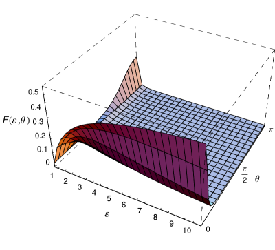
Figure 9: The universal function $F(\varepsilon,\theta)$ describing the excitation of the singlet $2^{1}S$ state of helium-like ion. The calculation is performed according to Eqs. (24) and (29) with respect to the dimensionless energy $\varepsilon$ of the incident electron and the scattering angle $\theta$.

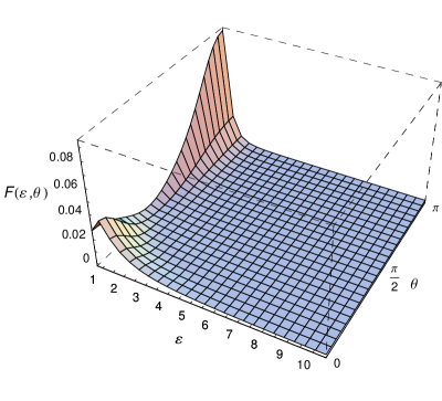
Figure 10: The universal function $F(\varepsilon,\theta)$ describing the excitation of the triplet $2^{3}S$ state of helium-like ion. The calculation is performed according to Eqs. (24) and (29) with respect to the dimensionless energy $\varepsilon$ of the incident electron and the scattering angle $\theta$.

Figure 11: The universal function $F(\varepsilon,\theta)$ is calculated according to Eqs. (24) and (29) for the particular scattering angle $\theta=0$ (forward scattering). Solid line, excitation into the singlet $2^{1}S$ state; dotted line, excitation into the triplet $2^{3}S$ state.

Figure 12: The universal function $F(\varepsilon,\theta)$ is calculated according to Eqs. (24) and (29) for the particular scattering angle $\theta=\pi$ (backward scattering). Solid line, excitation into the singlet $2^{1}S$ state; dotted line, excitation into the triplet $2^{3}S$ state.

Figure 13: The universal scaling $Q(\varepsilon)$ is presented as a function of the dimensionless energy $\varepsilon$ of the incident electron. Solid line, excitation into the singlet $2^{1}S$ state; dotted line, excitation into the triplet $2^{3}S$ state. The calculations are performed according to Eqs. (24), (27), and (29).

References

(1) R.J.W. Henry, Phys. Rep. 68 (1981) 1.
(2) Y. Itikawa, Phys. Rep. 143 (1986) 69.
(3) Y. Itikawa, Atomic Data Nucl. Data Tables 63 (1996) 315.
(4) V.I. Fisher, Y.V. Ralchenko, V.A. Bernshtam, A. Goldgirsh,
Y. Maron, L.A. Vainshtein, I. Bray, H. Golten, Phys. Rev.
A 55 (1997) 329.
(7) A.I. Mikhailov, I.A. Mikhailov, A.N. Moskalev,
A.V. Nefiodov, G. Plunien, G. Soff, Phys. Rev. A 69 (2004) 032703.
(8) K.T. Dolder, B. Peart, J. Phys. B 6 (1973) 2415.