Renormalisation in Quantum Mechanics

Abstract

This lecture provides an introduction to the renormalisation group as applied to scattering of two nonrelativistic particles. As well as forming a framework for constructing effective theories of few-nucleon systems, these ideas also provide a simple example which illustrates general features of the renormalisation group.

1 Effective theories

As particle and nuclear physicists, we are familiar with renormalisation in quantum field theory. We meet it first as a trick to get rid of mathematically unpleasant divergences. Later we learn to see it as part of a larger structure based on scale-dependence: the renormalisation group (RG). This is also how it appears in condensed-matter physics, in the context of critical phenomena [1].

The same ideas can also be used to study scale dependence in much simpler systems: just two or three nonrelativistic particles. They are of particular interest in nuclear physics, where we are trying to construct systematic effective field theories of nuclear forces (see [2] for recent reviews). They can also be applied to systems of cold atoms in traps, where magnetic fields can be used to tune the interactions between the atoms. In addition, these applications provide tractable examples of RG flows. Without the complications of a full field theory, the equations can often be solved exactly while still illustrating all of the general features of these flows [3].

Effective field theories describe only the low-energy degrees of freedom of some system and so they are not “fundamental”. In general they are not renormalisable and so they contain an infinite number of terms. This is potentially a disaster for their predictive power, but not if we can find a systematic way to organise these terms. Then, at any order in some expansion, only a finite number of terms will contribute. Having determined the coefficients of these by fitting them to data (or to simulations of the underlying physics), we can use them to predict other observables.

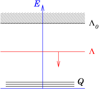
Figure 1: Scales and the running cut-off.

This works provided there is a good separation of scales, as illustrated in Fig. 1. Here $Q$ generically denotes the experimentally relevant low-energy scales and $\Lambda_{0}$ the scales of the underlying physics. In the case of nuclear physics, the low scales include particles’ momenta and the pion mass, while the high scales include the scale of chiral symmetry breaking, $4\pi f_{\pi}$, and the masses of hadrons like the $\rho$ meson and nucleon. If these are well separated, we can expand observables in powers of the small parameter $Q/\Lambda_{0}$. The terms in the effective theory can then be organised according to a “power counting” in the low scales $Q$.

The effective theory describes physics at low momenta. Short-range physics is not resolved by it and so is just represented by contact interactions ($\delta$-functions and their derivatives). However scattering by these is ill-defined since they couple to virtual states with arbitrarily high momenta. The basic nonrelativistic loop diagram (which is relevant for the rest of this talk) is shown in Fig. 2. For $S$-wave scattering this integral is

$$M\int\frac{q^{2}\,{\rm d}q}{p^{2}-q^{2}}\sim-M\int{\rm d}q,\quad\mbox{for large\ }q,$$ (1)

and so contains a linear divergence. We therefore need to regulate the theory. There are many ways to do this: dimensional regularisation [4], a simple momentum cut-off [3], or adding a term to the kinetic energy to suppress high-energy modes [5]. All of these are equivalent, but each introduces some arbitrary scale, $\Lambda$. This is essentially the highest momentum that is included explicitly in the theory. Physical predictions should be independent of $\Lambda$ and this leads us to the RG.

Figure 2: The basic loop integral.

As we lower $\Lambda$, the couplings must run. This is because more and more physics is “integrated out” (see Fig. 1) and so must be included implicitly in the effective couplings. Ultimately we lose all memory of the underlying physics and the only scale we have left is $\Lambda$. In units of $\Lambda$, everything is then just a number. We have arrived at a fixed point of the RG – a scale-free system. These are the end-points of the RG flow. Two are shown in Fig. 2. The one on the left is stable: any nearby theory will flow towards it as the the cut-off is lowered. In contrast, the one on the right has an unstable direction: the flow can take theories away from the fixed point unless they lie on the “critical surface”.

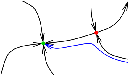
Figure 3: Fixed points.

Close to a fixed point, we can find perturbations that show a power-law dependence on $\Lambda$ and we can use this power counting to organise the terms in our effective theory. They can be classified into three types:

• $\Lambda^{-\nu}$: relevant/super-renormalisable,
  for example mass terms in quantum field theories like QED;

• $\Lambda^{0}$: marginal/renormalisable,
  for example the couplings familiar in gauge theories like the Standard Model (typically these show a $\log\Lambda$ dependence on the cut-off);

• $\Lambda^{+\nu}$: irrelevant/nonrenormalisable,
  for example the interactions in Chiral Perturbation Theory.

2 RG equation for two-body scattering

Let us look at scattering of two non-relativistic particles at low enough energies that the range of the forces is not resolved (for example, two nucleons with an energy below about 10 MeV). This can be described by an effective Lagrangian with two-body contact interactions or, equivalently, a Hamiltonian with a $\delta$-function potential. In momentum space, the $S$-wave potential can be written

$$V(k^{\prime},k,p)=C_{00}+C_{20}(k^{2}+k^{\prime 2})+C_{02}\,p^{2}\cdots,$$ (2)

where $k$ and $k^{\prime}$ denote the initial and final relative momenta and the energy-dependence is expressed in terms of the on-shell momentum $p=\sqrt{ME}$.

Scattering can be described by the reactance matrix ($K$), defined similarly to the scattering matrix ($T$) but with standing-wave boundary conditions. This has the advantage that it is real below the particle-production threshold. For $S$-wave scattering, it satisfies the Lippmann-Schwinger equation

$$K(k^{\prime},k,p)=V(k^{\prime},k,p)+\frac{M}{2\pi^{2}}\,{\cal{P}}\!\int_{0}^{\Lambda}q^{2}{\rm d}q\,\frac{V(k^{\prime},q,p)K(q,k,p)}{{p^{2}}-{q^{2}}},$$ (3)

where ${\cal P}$ denotes the principal value. This integral equation sums chains of the bubble diagrams in Fig. 2 to all orders. On-shell ($k^{\prime}=k=p$), the $K$-matrix is related to the $T$-matrix by

$$\frac{1}{K(p)}=\frac{1}{T(p)}-{\rm i}\,\frac{Mp}{4\pi}=-\,\frac{Mp}{4\pi}\,\cot\delta(p),$$ (4)

where $\delta(p)$ is the phase shift.

With contact interactions, the integral over the momentum $q$ of the virtual states is divergent and so we need to regulate it. Here I follow the method developed in [3] and simply cut the integral off at $q=\Lambda$. We can write the integral equation in the schematic form

$$K=V+VGK.$$ (5)

Demanding that the off-shell $K$-matrix be independent of $\Lambda$,

$$\dot{K}\equiv\frac{\partial K}{\partial\Lambda}=0,$$ (6)

ensures that scattering observables will be independent of the arbitrary cut-off. Differentiating the integral equation gives

$$0=\dot{V}+\dot{V}GK+V\dot{G}K,$$ (7)

where $\dot{G}$ implies differentiation with respect to the cut-off on the integral. Multiplying this by $(1+GK)^{-1}$ and using the integral equation for $K$, we arrrive at

$$\dot{V}=-V\dot{G}V.$$ (8)

This equation has a very natural structure: as states at the cut-off, with $q=\Lambda$, are removed from the loop integral in Fig. 2, their effects are added into the potential to compensate. Written out explicitly, it is

$$\frac{\partial V}{\partial\Lambda}=\frac{M}{2\pi^{2}}\,V(k^{\prime},\Lambda,p,\Lambda)\,\frac{\Lambda^{2}}{\Lambda^{2}-p^{2}}\,V(\Lambda,k,p,\Lambda).$$ (9)

Note that the use of the fully off-shell $K$-matrix was essential to obtaining an equation involving only the potential; a similar approach based on the half-off-shell $T$-matrix yields an equation that still involves the scattering matrix [6].

This equation for the cut-off dependence of the effective potential is still not quite the RG equation: the final step is to express all dimensioned quantities in units of $\Lambda$. Rescaled momentum variables (denoted with hats) are defined by $\hat{k}=k/\Lambda$ etc., and a rescaled potential by

$$\hat{V}(\hat{k}^{\prime},\hat{k},\hat{p},\Lambda)=\frac{M\Lambda}{2\pi^{2}}\,V(\Lambda\hat{k}^{\prime},\Lambda\hat{k},\Lambda\hat{p},\Lambda).$$ (10)

(The factor $M$ in this corresponds to dividing an overall factor of $1/M$ out of the Schrödinger equation.) This satisfies the RG equation

$$\Lambda\,\frac{\partial\hat{V}}{\partial\Lambda} = \hat{k}^{\prime}\,\frac{\partial\hat{V}}{\partial\hat{k}^{\prime}}+\hat{k}\,\frac{\partial\hat{V}}{\partial\hat{k}}+\hat{p}\,\frac{\partial\hat{V}}{\partial\hat{p}}+\hat{V}$$ (12)

$$\qquad+\hat{V}(\hat{k}^{\prime},1,\hat{p},\Lambda)\,\frac{1}{1-\hat{p}^{2}}\,\hat{V}(1,\hat{k},\hat{p},\Lambda).$$

The sum of logarithmic derivatives is similar to the structure of analogous RG equations in condensed-matter physics; it counts the powers of low-energy scales present in the potential. The boundary conditions on solutions to this equation are that they should be analytic functions of $\hat{k}^{2}$, $\hat{k}^{\prime 2}$ and $\hat{p}^{2}$ (since they should arise from an effective Lagrangian constructed out of $\partial/\partial t$ and $\nabla^{2}$). For small values of these quantities the potential should thus have an expansion in non-negative integer powers of them.

3 Fixed points and perturbations

Having constructed the RG equation, the first thing we should do is to look for fixed points – solutions that are independent of $\Lambda$. There is one obvious one: the trivial fixed point

$$\hat{V}=0.$$ (13)

(Since there is no scattering, this obviously describes a scale-free system.)

To describe more interesting physics, we need to expand around the fixed point, looking for perturbations that scale with definite powers of $\Lambda$. These are eigenfunctions of the linearised RG equation. They have the form

$$\hat{V}(\hat{k}^{\prime},\hat{k},\hat{p},\Lambda)=\Lambda^{\nu}\phi(\hat{k}^{\prime},\hat{k},\hat{p}),$$ (14)

and they satisfy the eigenvalue equation

$$\hat{k}^{\prime}\,\frac{\partial\phi}{\partial\hat{k}^{\prime}}+\hat{k}\,\frac{\partial\phi}{\partial\hat{k}}+\hat{p}\,\frac{\partial\phi}{\partial\hat{p}}+\phi=\nu\phi.$$ (15)

Its solutions are

$$\phi(\hat{k}^{\prime},\hat{k},\hat{p})=C\,\hat{k}^{\prime 2l}\,\hat{k}^{2m}\,\hat{p}^{2n},$$ (16)

with $k,l,m\geq 0$ since only non-negative, even powers satisfy the boundary condition. The corresponding eigenvalues are

$$\nu=2(l+m+n)+1.$$ (17)

These are all positive and so the fixed point is stable. The eigenvalues simply count the powers of low-energy scales. ($\nu=d+1$ where $d$ is the “engineering dimension”, as in Weinberg’s original power counting for ChPT [7].)

There are also many nontrivial fixed points, all of which are unstable. The most interesting one is purely energy-dependent. To study it, I focus on potentials of the form $V(p,\Lambda)$. The RG equation for these simplifies to

$$\Lambda\,\frac{\partial\hat{V}}{\partial\Lambda}=\hat{p}\,\frac{\partial\hat{V}}{\partial\hat{p}}+\hat{V}+\frac{\hat{V}(\hat{p},\Lambda)^{2}}{1-\hat{p}^{2}}.$$ (18)

Since all terms involve just one function, we can divide by $\hat{V}^{2}$ to get

$$\Lambda\,\frac{\partial}{\partial\Lambda}\left(\frac{1}{\hat{V}}\right)=\hat{p}\,\frac{\partial}{\partial\hat{p}}\left(\frac{1}{\hat{V}}\right)-\frac{1}{\hat{V}}-\frac{1}{1-\hat{p}^{2}},$$ (19)

which is just a linear equation for $1/\hat{V}(\hat{p},\Lambda)$.

To find the fixed point, we set the LHS of this equation to zero. The resulting ODE can then be integrated easily. The general solution is

$$\frac{1}{\hat{V}_{0}(\hat{p})}=-\int_{0}^{1}\frac{\hat{q}^{2}\,{\rm d}\hat{q}}{\hat{q}^{2}-\hat{p}^{2}}+C\hat{p}.$$ (20)

The final term is not analytic in $\hat{p}^{2}$ and so the boundary condition requires $C=0$. The fixed-point potential is thus

$$\frac{1}{\hat{V}_{0}(\hat{p})}=-1+\frac{\hat{p}}{2}\ln\frac{1+\hat{p}}{1-\hat{p}}.$$ (21)

The precise form of this is regulator-dependent (for example, it is just a constant for dimensional regularisation [4]), but the presence of a negative constant of order unity is generic.

Since this potential has no momentum dependence, the integral equation for the $K$-matrix simplifies to an algebraic equation. In rescaled, dimensionless form, it can be written

$$\frac{1}{\hat{K}(\hat{p})}=\frac{1}{\hat{V}_{0}(\hat{p})}-\int_{0}^{1}\frac{\hat{q}^{2}\,{\rm d}\hat{q}}{\hat{p}^{2}-\hat{q}^{2}}.$$ (22)

The integral here is just the negative of the one above in $1/\hat{V}_{0}$ itself and so we get

$$\frac{1}{\hat{K}(\hat{p})}=0.$$ (23)

The corresponding $T$-matrix,

$$\frac{1}{\hat{T}(\hat{p})}=\frac{1}{\hat{K}(\hat{p})}+{\rm i}\,\frac{\pi}{2}\,\hat{p},$$ (24)

has a pole at $\hat{p}=0$. The fixed-point therefore describes a system with a bound state at exactly zero energy (another scale-free system).

More general systems can be described by perturbing around the fixed point. In particular, energy-dependent perturbations can be found by substituting

$$\frac{1}{\hat{V}(\hat{p},\Lambda)}=\frac{1}{\hat{V}_{0}(\hat{p})}+\Lambda^{\nu}\phi(\hat{p})$$ (25)

into the RG equation. The functions $\phi(\hat{p})$ satisfy the eigenvalue equation

$$\hat{p}\,\frac{\partial\phi}{\partial\hat{p}}-\phi=\nu\phi.$$ (26)

The solutions to this are powers of the energy,

$$\phi(\hat{p})=C\hat{p}^{2n},$$ (27)

with eigenvalues

$$\nu=2n-1.$$ (28)

The RG eigenvalues for these perturbations have been shifted by $-2$ compared to the simple “engineering” power counting. There is one negative eigenvalue and so the fixed point is unstable.

A slice through the RG flow is shown in Fig. 4. The two fixed points can be seen, as well as the critical line through the nontrivial one. Potentials close to this line initially flow towards the fixed point as we lower the cut-off but are then diverted away from it. A potential to the right of the line is not quite strong enough to produce a bound state. As $\Lambda$ passes through the scale associated with the virtualstate, the flow turns to approach the trivial fixed point from the weakly attractive side. In contrast, a potential to the left of the critical line generates a finite-energy bound state. This state drops out of our low-energy effective theory when the cut-off reaches the corresponding momentum scale. As this happens, the RG flow takes the potential to infinity and it then reappears from the right, ultimately approaching the trivial fixed point from the weakly repulsive side.

Figure 4: RG flow of the potential $\hat{V}(\hat{p},\Lambda)=b_{0}(\Lambda)+b_{2}(\Lambda)\,\hat{p}^{2}+\cdots$.

Exercise: Repeat this analysis for a general number of space dimensions, in particular for $D=1$ and 2, and interpret your results.

Physical observables are given by the on-shell $K$-matrix. Returning to physical units, this is

$$\frac{1}{K(p)}=\frac{M}{2\pi^{2}}\sum_{n=0}^{\infty}C_{n}\,p^{2n},$$ (29)

where the $C_{n}$ are the coefficients of the RG eigenfunctions in $1/\hat{V}$. Comparing this with

$$\frac{1}{K(p)}=-\,\frac{Mp}{4\pi}\left(-\,\frac{1}{a}+\frac{1}{2}\,r_{e}p^{2}+\cdots\right),$$ (30)

we see that this expansion is, in fact, just the effective-range expansion (first applied to the nucleon-nucleon interaction by Bethe in 1949 [8]). Note that the terms in the expansion of our effective theory have a direct connection to scattering observables. This is as it should be: effective theories are systematic tools to analyse data, not fundamental theories that aim to predict everything in terms of a small number of parameters.

Finally, I should make a brief comment about momentum-dependent perturbations around the nontrivial fixed point, which I have not discussed above. These terms change the off-shell dependence of the scattering matrix, without affecting physical observables. Their explicit forms can be found in Ref. [3]. In contrast to the expansion around the trivial fixed point, momentum- and energy-dependent terms appear at different orders. Specifically, the momentum-dependent perturbations around the nontrivial point have even RG eigenvalues. Each term is one order higher in the expansion than the corresponding energy-dependent one. This means that using them to eliminate energy dependence will leave an effective potential without an obvious power counting (like the potential obtained in Ref. [6]).

4 Extensions

Here I have discussed only the application of the RG to systems where the range of the forces is not resolved and the interactions can all be represented by contact terms. There are many other systems with known long-range forces, for example: Coulomb, pion exchange, dipole-dipole or van der Waals interactions. Similar RG methods can be applied to the unresolved short-range forces accompanying these [9, 10]. The resulting expressions are either distorted-wave Born expansions or distorted-wave versions of the effective-range expansion. (In the case of the Coulomb potential, it was again Bethe who first wrote this expansion down [8].)

Another important application is to the $1/r^{2}$ potential that arises in three-body systems with attractive short-range forces [11]. If the two-body scattering length is infinite, the Efimov effect leads to a tower of geometrically-spaced bound states [12]. This is the origin of the limit cycle that has been found in the RG flows for these systems [13] (one of the few known examples of such a cycle).

References

- [1] K. G. Wilson, Rev. Mod. Phys. 55 (1983) 583.
- [2] P. F. Bedaque and U. van Kolck, Ann. Rev. Nucl. Part. Sci. 52 (2002) 339 [nucl-th/0203055]; E. Epelbaum, Prog. Part. Nucl. Phys. 57 (2006) 654 [nucl-th/0509032].
- [3] M. C. Birse, J. A. McGovern and K. G. Richardson, Phys. Lett. B464, 169 (1999) [hep-ph/9807302].
- [4] Nucl. Phys. B534 (1998) 329 [nucl-th/9802075].
- [5] K. Harada, H. Kubo and A. Ninomiya, nucl-th/0702074.
- [6] S. K. Bogner, A. Schwenk, T. T. S. Kuo and G. E. Brown, nucl-th/0111042; see also: S. K. Bogner et al., Phys. Lett. B576 (2003) 265 [nucl-th/0108041].
- [7] S. Weinberg, Physica A96 (1979) 327; Phys. Lett. B251 (1990) 288.
- [8] H. A. Bethe, Phys. Rev. 76 (1949) 38.
- [9] T. Barford and M. C. Birse, Phys. Rev. C67 (2003) 064006 [hep-ph/0206146].
- [10] M. C. Birse, Phys. Rev. C74 (2006) 014003 [nucl-th/0507077].
- [11] T. Barford and M. C. Birse, J. Phys. A: Math. Gen. 38 (2005) 697 [nucl-th/0406008].
- [12] V. N. Efimov, Sov. J. Nucl. Phys. 12 (1971) 589; 29 (1979) 546.
- [13] P. F. Bedaque, H.-W. Hammer and U. van Kolck, Phys. Rev. Lett. 82, 463 (1999) [nucl-th/9809025]; Nucl. Phys. A646, 444 (1999) [nucl-th/9811046]; Nucl. Phys. A676, 357 (2000) [nucl-th/9906032].