Simulation Studies and Detector Scenarios
for an ILC Polarimeter

Abstract

High energy longitudinal electron polarimetry will be based on Compton scattering for the International Linear Collider. An unobtrusive measurement has to include a magnet chicane setup serving as a spectrometer. Current proposals make use of Cerenkov detectors for electron detection. A fast simulation has been developed to study the basic properties of scenarios for the polarimeter setup.

1 Introduction

Electron polarimetry at the International Linear Collider (ILC) will be based on Compton scattering using a laser colliding head-on with the incident lepton beam in the beam delivery system. The shape of the differential Compton cross section depends strongly on the helicity states of electron beam and laser. Asymmetries can then be determined from different helicity configurations, which scale with the longitudinal polarization of the electron bunches [2].

At ILC energies of 250 GeV or more, the angular distributions of both the scattered photons and the recoil electrons are constrained to within a few $\mu$rad for all but the most highly energetic photons. The polarimeter, therefore, will be placed in a magnet chicane serving as a spectrometer for the recoil electrons (see figure 1). The setup consists of four sets of dipoles in such a way that the emittance of the incident electron beam should not be impaired by more than 1%. The electrons are first displaced parallel to their original direction by about 2 cm to the side by two sets of dipoles. After that, a pulsed laser (10 ps with 35 $\mu$J) hits the bunches head-on

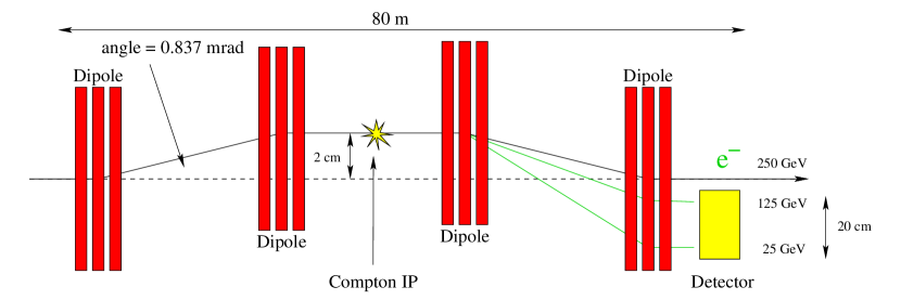
Figure 1: Proposed layout of the upstream electron polarimeter in a magnet chicane.

and deflects about $10^{3}$ out of the $20\cdot 10^{9}$ electrons. The second pair of dipole sets puts the undisturbed electrons back on their original track and serves as a spectrometer for the recoil particles which are deflected more strongly due to their reduced energy.

The Compton electron yield will then be determined after the last dipole set in a Cerenkov detector. The detector needs to cover less than 20 cm horizontally and only a fraction of that in vertical direction due to the orientation of the dipoles. The overall length of the polarimeter is reaching almost 80 m to accomplish this spread and to comply with the accelerator emittance demands at the same time. Cerenkov light will be produced by the electrons in gas tubes or quartz fibers, alternatively. The light is then transferred further to photo-detectors which are placed out of the accelerator plane in order to reduce background from beam related interaction or other effects from the beam delivery system.

The polarimeter location and setup have to be chosen carefully, since the polarization needs to be known as close to the electron-positron interaction point as possible. Especially the direction of the polarization vector can change easily in the magnetic fields of the beam delivery system. Beam orbit alignment accuracies have been estimated to be smaller than 80 $\mu$rad at 250 GeV for the measurement to be in compliance with the physics demands for the polarization determination ($\Delta P/P\leq 0.25\%$, [2, 3]). The polarimeter setup is such that the Compton edge does not change its position in the detector with respect to the incident beam energy. This is especially of value during commissioning of the accelerator in order to keep track of polarization preservation and also in threshold scans.

2 Fast Simulations

A fast Monte Carlo simulation has been developed which is used for first analyses of the basic properties of the polarimeter layout and the detector design. Bunches of $20\cdot 10^{9}$ electrons at 250 GeV and 80% polarization are coupled to the circularly polarized, green laser pulses (2.33 eV) by a Compton generator. Both beams have an assumed circularly distributed width with a gaussian shape of $\sigma$ = 50 $\mu$m. Also, there is a slight crossing angle of 10 mrad which is necessary in the experimental setup later.

The Compton recoil electrons are tracked through the dipoles and translated into Cerenkov photons at the location of the detector through a refraction index of 1.0014 for $C_{4}F_{10}$ or pressurized propane (1.1 atm). Light transmission to the photo-detectors is currently covered by a global efficieny of 55%.

The light yield detected by the photo-detectors is determined from the wavelength dependent quantum efficiency. It has been taken from conventional Hamamatsu R6094 photo-multiplier tubes. Between 300 nm $\leq\lambda\leq$ 650 nm, the quantum efficiency reaches a maximum of 25% around 350 nm and drops to zero elsewhere due to the opacity of the entrance window glass. Adc-counts are finally derived from the detected photons. These counts can be distorted by a quadratic function that describes the general behaviour of differential non-linearities in the electronics read-out chain. The distortion is maximal for medium values and vanishes at zero counts and when reaching saturation level.

The Adc-counts are determined for same and opposite helicity configurations and accumulated over several bunches. From these, an asymmetry is calculated as a function of channel number, see left side of figure 2. The channel number reflects the transverse position of the Compton electrons at the detector surface (2 cm $\leq x\leq$ 20 cm) and is, therefore, a function of the inverse recoil energy.

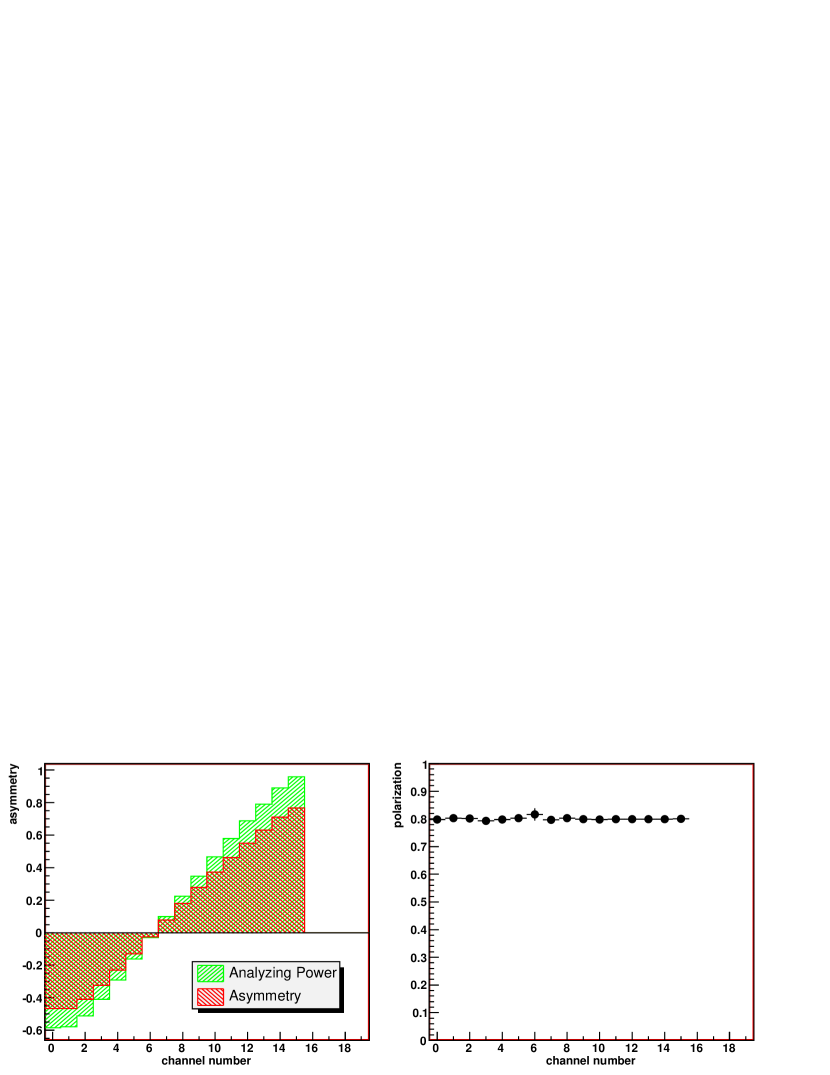
Figure 2: Asymmetry $\epsilon$ and analyzing power $A$ as functions of channel number. The ratio of both leads to the electron longitudinal polarization $P$.

The polarization $P$ is calculated from the measured asymmetry $\epsilon$ and the calculated analyzing power $A$, i.e., the Compton asymmetry for completely polarized electron bunches:

$$\epsilon=A\cdot P=\frac{N^{+}_{\sc Adc}-N^{-}_{\sc Adc}}{N^{+}_{\sc Adc}+N^{-}_{\sc Adc}},$$ (1)

where $N^{+}_{\sc Adc}$ and $N^{-}_{\sc Adc}$ are the integrated Adc-counts.

Polarizations are determined for each channel seperately and then combined to a weighted mean (see right side of figure 2). This way, problematic channels can be excluded from the average value, which is especially important for the zero crossing of the asymmetry (channel 6 in figure 2). Statistical errors diminish after accumulation over many bunch trains of each 2820 bunches and reveal systematic uncertainties.

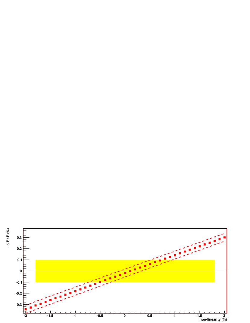
Figure 3: Effect of electronics differential non-linearities on the determination of the electron polarization. The yellow box represents the range of the desired maximum contribution to the total error $\Delta P/P\leq 0.25\%$.

Experimentally, the polarization will be extracted from the output Adc-counts without proper knowledge of integral or differential non-linearities. In the simulation, one can compare the experimental values with the primary Compton electrons or with the secondary Cerenkov photons, so the effect of the distorted Adc-readout becomes traceable for single channels. Also, the measured polarization can be checked with respect to the real (input) electron polarization. Figure 3 shows the deviations between measured and real polarizations as a function of the quadratic non-linearities for a 20-channel detector.

In order to meet the physics demand for the polarization measurement, it is necessary to be in control of differential non-linearities in the range of 0.5%, contributing less than 0.1% to $\Delta P/P$. This effect is decreasing with increasing channel numbers. However, for Cerenkov tubes, a channel width of 1 cm seems to be a reasonable size. First non-linearity measurements have been carried out in a test stand [4] and more detailed studies of the whole detector setup are planned.

3 Outlook

The simulation so far is very limited and only includes non-linearities of the electronics read-out after tracking the Compton electrons towards the detector surface and transforming them into Cerenkov photons. In the future, a full picture of the polarimeter has to include other details of the magnet chicane and the detector setup. This includes a proper description of the gas (or possibly other) volumes, the geometry for the transmission with reflectivities and absorption, and light extraction in the photo-detectors. There are on-going efforts to use Bdsim [5] for a description of the magnet chicane and add an accurate Geant4 model of the complete detector setup. This simulation would also serve as a comprehensive tool to study the possibilities of combining the beam emittance measurement or others with the polarimeter chicane. Such an additional measurement might induce additional downstream background which has to be considered carefully.

4 Acknowledgments

The authors acknowledge the support by DFG Li 1560/1-1.

References

-
[1]
Slides:
http://ilcagenda.linearcollider.org/materialDisplay.py?contribId=173&sessionId=78&confId=1296 - [2] V. Gharibyan, N. Meiners and P. Schüler, LC-DET-2001-047 (2001) and references therein.
- [3] G. Mortgaat-Pick et al., CERN-PH-TH/2005-036 and references therein.
- [4] D. Käfer et al., these proceedings (2007).
-
[5]
http://cvs.pp.rhul.ac.uk/cvsweb.cgi/BDSIM/docs/