The interaction of planetary nebulae and their AGB progenitors with the interstellar medium

Abstract

Interaction with the Interstellar Medium (ISM) cannot be ignored in understanding planetary nebula (PN) evolution and shaping. In an effort to understand the range of shapes observed in the outer envelopes of PNe, we have run a comprehensive set of three-dimensional hydrodynamic simulations, from the beginning of the asymptotic giant branch (AGB) superwind phase until the end of the post–AGB/PN phase. A ’triple-wind’ model is used, including a slow AGB wind, fast post–AGB wind and third wind reflecting the linear movement through the ISM. A wide range of stellar velocities, mass-loss rates and ISM densities have been considered.

We find ISM interaction strongly affects outer PN structures, with the dominant shaping occuring during the AGB phase. The simulations predict four stages of PN–ISM interaction whereby the PN is initially unaffected (1), then limb-brightened in the direction of motion (2), then distorted with the star moving away from the geometric centre (3) and finally so distorted that the object is no longer recognisable as a PN and may not be classed as such (4). Parsec-size shells around PN are predicted to be common. The structure and brightness of ancient PNe is largely determined by the ISM interaction, caused by rebrightening during the second stage; this effect may address the current discrepancies in Galactic PN abundance. The majority of PNe will have tail structures. Evidence for strong interaction is found for all known planetary nebulae in globular clusters.

1 Introduction

Planetary nebulae (PNe) display a wide variety of shapes ranging from round, which can be simply understood in terms of the symmetric interacting stellar winds (ISW) model (Kwok, 1982), through complex symmetrical shapes, such as hour-glasses and butterflies, to shapes which have only rotational point-symmetry. Many theories have been introduced to explain these complex shapes from adding an asymmetric slow wind to the ISW model (Kahn, 1985; Balick, 1987) to involving the effects of binary central stars (Soker, 1996) and magnetic fields (Frank & Blackman, 2004). Observations of PNe have shown several cases where only the outer shell shows a departure from symmetry. In these cases, the cause of the asymmetries has been postulated to be an interaction with the interstellar medium (ISM).

Interaction with the ISM by PNe was first discussed by Gurzadyan (1969) with an early theoretical study by Smith (1976) employing the ’snow-plough’ model of Oort (1951). Smith concluded that a nebula will fade away before any disruption of the nebular shell becomes noticable. Isaacmann (1979) used the same approximation with higher relative velocities to the ISM and ISM densities and concluded similarly.

In contrast, Borkowski et al. (1990) found that many PNe with large angular extent show signs of PN–ISM interaction and that all nebulae containing central stars with a proper motion greater than 0.015 arcsec yr^-1 do so. Soker et al. (1991) hydrodynamically modelled the interaction revealing that the PN shell is first compressed in the direction of motion and then in later stages this part of the shell is significantly decelerated with respect to the central star. Both conclude that the interaction with the ISM becomes dominant when the density of the nebular shell has dropped below a certain critical limit, typically $n_{\rm H}=40$ cm^-3 for a PN in the Galactic plane. These low densities require large, evolved nebulae, in agreement with the observational result of Borkowski et al. (1990). They noted that their simple picture breaks down for high velocity PNe in a low density environment. Here, a Rayleigh–Taylor (RT) instability develops, leading to shell fragmentation. Their 2D hydrodynamic simulations started with the nebula shell already formed but above their upper density limit for ISM interaction to become apparent.

The fragmentation predicted by Soker et al. (1991) was discussed in more depth by Dgani & Soker (1994) and then Dgani & Soker (1998). In these papers, Dgani and Soker applied theoretical results of hydrodynamic instabilities and found that the RT instability can play an important role in the shaping of the outer regions of a PN. They suggested these RT instabilities can cause fragmentation of the bow shock with Kelvin–Helmholtz instabilities also playing a part. Any fragmentation caused by these instabilities would only be present if the relative velocity to the ISM of the central star was greater than 100 $\mathrm{km\,s}^{-1}$.

Villaver et al. (2003) (hereafter referred to as VGM) pointed out that the PN–ISM interaction had previously been studied by considering the interaction after the nebular shell had formed. PNe are formed when a slow wind ($\sim 10$ $\mathrm{km\,s}^{-1}$) ejected during the preceding asymptotic giant branch (AGB) phase of evolution is swept up into a dense shell by a fast wind ($\sim 10^{3}$ $\mathrm{km\,s}^{-1}$) from the exposed, ionizing hot white dwarf core. VGM performed 2D hydrodynamic simulations and found that crucially the interaction begins during the AGB phase where the slow wind is shaped by the ISM. The PN forms in this pre-shaped environment. Choosing a conservative relative velocity of the central star to the ISM of 20 $\mathrm{km\,s}^{-1}$ and a low density of the surrounding ISM of $n_{\rm H}=0.1$ cm^-3, they discovered that the PN is brightened on the upstream side of the nebular shell. They concluded that PN–ISM interaction provides an adequate mechanism to explain the high rate of observed asymmetries in the external shells of PNe. Further, stripping of mass downstream during the AGB phase provides a possible solution to the problem of missing mass in PN whereby only a small fraction of the mass ejected during the AGB phase is inferred to be present during the post–AGB phase. Observational evidence for the effect of the ISM on AGB wind stuctures, supporting VGM’s findings was found by Zijlstra & Weinberger (2002).

VGM found that simple hydrodynamic simulations can reveal much information regarding the PN–ISM interaction. In order to investigate the interaction further, we have developed a ’triple-wind’ model including an initial slow AGB wind, a subsequent fast post–AGB wind, and a third continuous wind reflecting the movement through the ISM. Employing a parallel 3D hydrodynamic scheme developed by Wareing (2005), we have understood the formation of the extreme PN Sh 2-188 (Wareing et al., 2006a) and the structure around the AGB star R Hya (Wareing et al., 2006b).

Sh 2-188 was thought to be a bright one-sided arc-like PN when new observations taken as part of the Isaac Newton Group Photometric H$\alpha$ Survey of the Northern Galactic Plane (IPHAS) (Drew et al., 2005) revealed a faint ring-like completion of the arc and a tail stretching away in opposition to the bright arc. Our model revealed this PN to be a strong PN–ISM interaction where the central star is moving at 125 $\mathrm{km\,s}^{-1}$ in the direction of the bright arc relative to the ISM and the nebular shell is interacting with a bow shock formed during the AGB phase between the slow wind and the ISM. Recent IR observations of the AGB star R Hya as part of the MIRIAD programme (Ueta et al., 2006) have revealed the arc-like structure to the North West of the star to be a bow shock ahead of the star (Wareing et al., 2006b). The existence of this AGB wind bow shock has confirmed the hypothesis that the major shaping effect for the PN–ISM interaction occurs during the AGB phase of evolution.

Using our model, we have now run a comprehensive set of 92 simulations equivalent to over 5 years of single CPU computation time investigating the PN–ISM interaction. In this paper, we discuss a representative set of these simulations and generalise the interaction into four distinct stages, indicating its effect on shaping and other PN characteristics. We apply our generalisation to a selection of PNe from the IAC Morphological Catalog of Northern Galactic Planetary Nebulae (Manchado et al., 1996) and find indications of interaction with the ISM in approximately 20 per cent of objects.

2 The hydrodynamic scheme and triple-wind model

The numerical scheme, CUBEMPI, used in our simulations to solve the hydrodynamics equations employs a second-order Godunov solution due to Falle (1991). In recent years, variants of CUBEMPI have been used to shed light on nova explosions (Lloyd et al., 1997; Porter et al., 1998), extragalactic jet-cloud interactions (Higgins et al., 1999) and most recently PN (Mitchell, 2007; Wareing et al., 2006a). The version of the scheme used here is posed in 3D cartesian coordinates, fully parallel and includes the effect of radiative cooling due to the cooling curves of Raymond et al. (1976) above 10⁴ K as the cooling curves extend no further. The parallelisation was developed using the MPI library and involves slicing the numerical domain along an axis and communicating relevant boundary data at the correct points during a computational timestep. The parallelisation has been successfully tested for efficiency and scalability. The scheme itself has also been tested on a number of standard computational fluid dynamics problems and performed well on all tests. It has been further tested using astrophysical problems which have highlighted its capability for shock capturing, an important requirement for the modelling of PNe. The parallelisation and testing are detailed in Wareing (2005)

The numerical domain consists of a cubic grid, 200 cells along each axis, containing a total of $8\times 10^{6}$ uniformly-spaced cells. The grid is sliced ten times for parallelisation purposes and distributed across ten processors of the COBRA beowulf-type supercomputer at Jodrell Bank. This level of parallel distribution is a comprimise between computational efficiency and availability of computational resources.

In the ’triple-wind’ model, the simulation is performed in the frame of reference of the star, which is placed at cell coordinates ($50,100,100$). Mass loss is effected by setting the values of hydrodynamic variables (density, momentum density and energy density) in a volume-weighted spherical region of radius 5$\frac{3}{4}$ cells centred on the star. The radius of this source volume has been chosen by an experimental process balancing production of the most spherical PN when modelling the stationary ISW model with spherically symmetric winds (i.e. reducing the pixelation of the cartesian grid) and avoidance of interference with results of the simulation. The conditions within the source volume are reset at the beginning of every computational timestep to drive the ejection of the wind. The wind has been modelled with a spherically symmetric constant mass-loss rate $\dot{M}$ with constant velocity $v$ and temperature $T$. Density in the source volume has been defined by $\dot{M}/(4\pi vr^{2})$ where $r$ is the physical radial distance from the central star. The other hydrodynamic variables are set accordingly. Simulation of movement through the ISM is achieved by flowing ISM material in at the ($x=1$) boundary with a velocity vector v_x, v_y, v_z = ($+v$,0,0). The ISM density and temperature are constant. All other numerical boundaries have conditions allowing material to flow out of the domain freely. Gas pressures in the model are calculated assuming an ideal gas equation of state.

3 Model parameters

In our simulations, we have held the following parameter values constant: for the slow AGB wind a velocity of $v_{\rm sw}=15$ $\mathrm{km\,s}^{-1}$ and a temperature of $T_{\rm sw}=10^{4}$ K as the cooling curves extend no further; for the fast post–AGB wind a mass-loss rate of $\dot{M}_{\rm fw}=5\times 10^{-8}$ $\mathrm{M_{\odot}\,yr}^{-1}$, a velocity of $v_{\rm fw}=1000$ $\mathrm{km\,s}^{-1}$ and a temperature of $T_{\rm fw}=5\times 10^{4}$ K; and for the ISM a temperature of $T_{\rm ISM}=8000$ K, characteristic of the warm intercloud medium (Burton, 1988). These parameter values are typical of observations of PN conditions. In the model, the switch between the AGB wind and the post–AGB wind is instantaneous and occurs after $5\times 10^{5}$ years of AGB evolution, typical of the duration of this phase. In view of the still considerable uncertainties on the detailed properties and evolution of these winds, more detailed temporal variations have not been modelled. We have discussed this further in later sections.

In our simulations, we have varied three parameters: relative velocity of the star to the surrounding ISM $v_{\rm ISM}$, slow wind mass-loss rate $\dot{M}_{\rm sw}$ and ISM density $\rho_{\rm ISM}$. Binney & Merrifield (1998) discussed $v_{\rm ISM}$ of stars in the Galactic plane: typical thin disk stars resulting in a PN appear to have a transverse variation on their galactic rotation velocity of 35 – 50 $\mathrm{km\,s}^{-1}$; thick disk stars, rarer in the Galactic plane, have a typical range of 50 – 75 $\mathrm{km\,s}^{-1}$; halo objects can have a typical variation greater than 100 $\mathrm{km\,s}^{-1}$. Older stellar groups, such as PNe, are characterized by larger velocity dispersions and asymmetric drift velocities than are younger stellar groups. The average transverse motions of stars in the solar neighbourhood have been found to be in the range of 20–40 $\mathrm{km\,s}^{-1}$ with the tail of the distribution up to 130 $\mathrm{km\,s}^{-1}$ (Skuljan et al., 1999). For white dwarfs an average velocity of $67.4\pm 39.5$ $\mathrm{km\,s}^{-1}$ has been found by Sanggak (1984). In terms of Galactic disk PNe, Borkowski et al. (1990) state 60 $\mathrm{km\,s}^{-1}$ as an average velocity. For Galactic Bulge PNe, velocities up to 200 $\mathrm{km\,s}^{-1}$ could be reasonably expected as these stars are dynamically a much hotter population. Therefore, we have considered a range of $v_{\rm ISM}$ from 0 $\mathrm{km\,s}^{-1}$, testing the implementation of the triple-wind model and its ability to simulate a spherical nebula, up to 200 $\mathrm{km\,s}^{-1}$, in 25 $\mathrm{km\,s}^{-1}$ steps in order to fully cover the range of velocities of PN-forming stars in the Galaxy.

The typical density of the ISM in the galactic plane is approximately $n_{\rm H}$ = $\sim 2$ cm^-3 up to a scale height of 100 pc above the plane where it then begins to drops off exponentially. We have used three constant values of ISM density $n_{\rm H}$ = 2, 0.1 & 0.01 cm^-3 to investigate this range. These densities are comparable to that of the warm intercloud medium (Burton, 1988).

Mass-loss rates during the AGB phase of evolution vary between 10^-7 – 10^-6 $\mathrm{M_{\odot}\,yr}^{-1}$ with brief periods of enhanced mass-loss up to 10^-5 $\mathrm{M_{\odot}\,yr}^{-1}$. As we are using a constant mass-loss rate, we have not modelled mass-loss variations. We have used values of 10^-7, $5\times 10^{-7}$, 10^-6 & $5\times 10^{-6}$ $\mathrm{M_{\odot}\,yr}^{-1}$ up to $v_{\rm ISM}$ = 75 $\mathrm{km\,s}^{-1}$. Above this velocity, we have not used a mass-loss rate of 10^-6 $\mathrm{M_{\odot}\,yr}^{-1}$ due to time and computational constraints.

4 Results

In our initial test cases $v_{\rm ISM}$ is set to zero. The forward shock driven by the AGB wind is spherical and expands into a homogeneous ISM. The shocked ISM material behind the forward shock is of relatively low density with the contact discontinuity and the reverse shock expanding spherically symmetrically outward. The unshocked AGB wind behind the reverse shock is also spherically symmetric around the central star with an approximate 1/r² distribution. After 500 000 years, the fast post–AGB wind is introduced into this distribution driving a shock which sweeps up the AGB wind material into an expanding shell. The shell has a relatively high density and a temperature on the scale of 10–20 000 K. The stromgren sphere around the central star encompasses the shell indicating the material in the shell would be ionized and observable as a PN. This method of PN formation is the result of interacting stellar winds and is the premise of the ISW model.

Next, we added the ISM velocity. We display and discuss a representative set of five simulations covering various parameter values which serve to illustrate the range of PN structures formed in all our simulations. Table 1 shows the parameter values for these five simulations. The resulting PN structure is discussed for each case. In our online supplementary appendix, we have also included snapshots at the end of the AGB phase of evolution and parameter values for our full set of simulations. We have performed calculations to find the extent of the stromgren sphere during the PN phase and find that in all cases it extends beyond the simulation domain.

In the following figures, the results are illustrated by slices through the density data cubes at the position of the central star and parallel to the direction of motion.

Table 1: Input parameters for the five selected simulations discussed in section 4. Column a) gives the simulation reference; column b) $v_{\rm ISM}$; column c) the density of the surrounding ISM in $n_{\rm H}\,\rm cm^{-3}$; column d) the constant mass-loss rate during the AGB phase of evolution; and column e) the physical size of the grid along one dimension of the numerical domain.

a)	b)	c)	d)	e)
case	$v_{\rm ISM}$	ISM:$n_{\rm H}$	$\dot{M}_{\rm sw}$	Grid
	($\mathrm{km\,s}^{-1}$)	(cm-3)	(M⊙ yr-1)	(pc)
A	25	0.01	$5\times 10^{-7}$	23.4
B	50	2	$5\times 10^{-6}$	2.6
C	75	2	$5\times 10^{-6}$	1.75
D	100	2	$10^{-7}$	1.0
E	125	2	$5\times 10^{-6}$	1.0

4.1 Case A

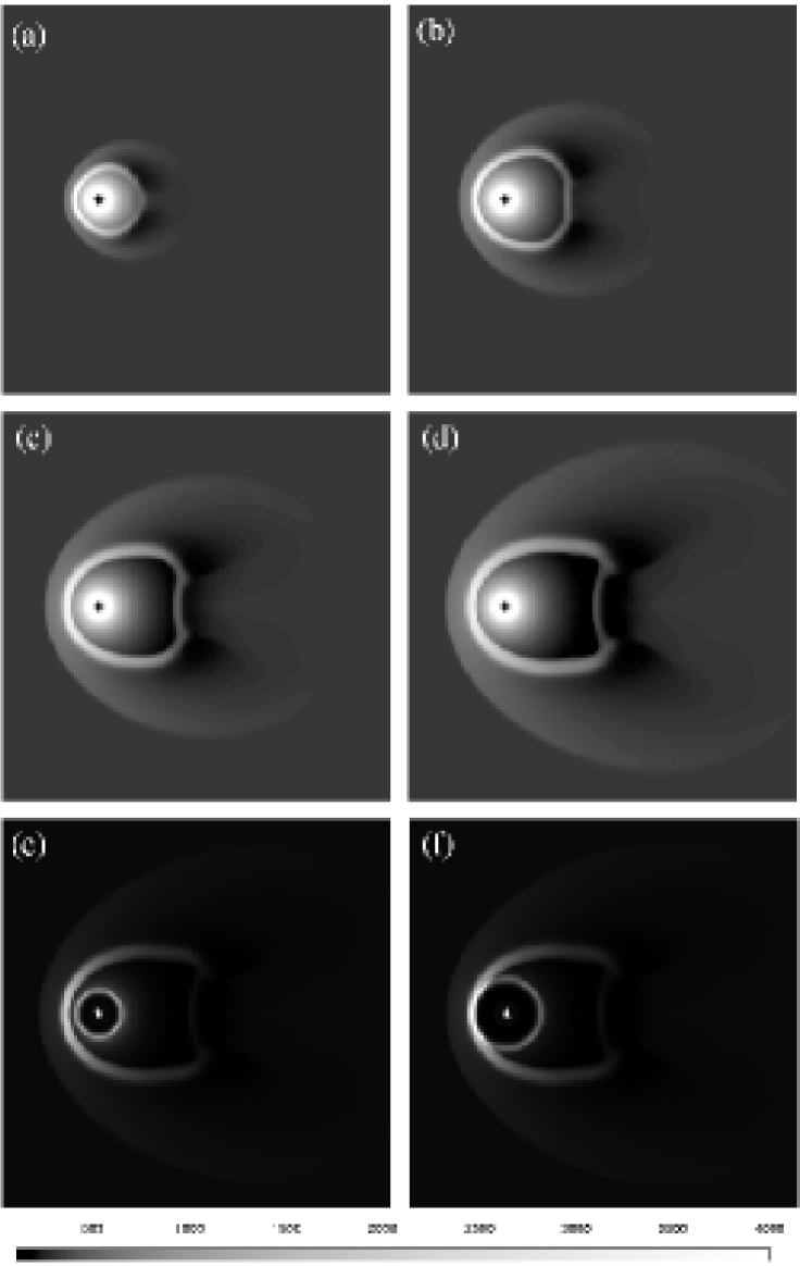
Figure 1: The results of case A: the panels show the gas density during the AGB and post–AGB phases. In panel (a), the simulation is 125 000 years into the AGB phase, panel (b) 250 000 years, panel (c) 375 000 years, panel (d) 500 000 years, panel (e) 15 000 years into the post–AGB phase and in panel (f) 30 000 years. The position of the central star is marked by an asterisk. The colour scaling is logarithmic and the density is scaled in units of $10^{-6}\ \mathrm{M_{\odot}\,pc}^{-3}$ where 25 000 is equivalent to $n_{\rm H}$ = 1.0 cm^-3.

Figure 1 shows the result of case A. The central star has $v_{\rm ISM}$ of 25 $\mathrm{km\,s}^{-1}$. The AGB evolution is shown in the top four panels (a)–(d) with the post–AGB evolution in the bottom two panels (e) and (f). In panel (a), 125 000 years into the AGB phase, the shock has formed into a bow shock a short distance upstream of the central star with a tail connecting a short distance downstream of the central star. Over the next three panels (b), (c) and (d), at 250 000, 375 000 and 500 000 years respectively, the bow shock can be seen to expand outwards from the central star and between panels (c) and (d) reach a stable position ahead of the star. This can be understood in terms of a ram pressure balance between the slow wind and the oncoming ISM. At this point, the bow shock is approximately 2.5 pc ahead of the central star. If we assume this is a strong shock, the temperature of the shocked material at the head of the bow shock should be equal to (3/16) (m $v_{\rm ISM}$²/k) where $m$ is the particle mass in the simulation and $k$ the Boltzmann constant. Our simulation is in agreement with this. The tail structure can be understood in terms of material being ram-pressure stripped from the head of the bow shock and cooling as it flows downstream around the bow shock into the tail. It is clear that even at this low speed, the ISM interaction strongly affects the shape of the AGB wind.

The brightest phase of the PN evolution, typically 1–5$\times 10^{3}$ yr into the post–AGB phase, is not shown. Panel (e) shows the phase 15 000 years into the post–AGB phase. The expanding (and now faint) shell of the PN is clear, inside and still detached from the bow shock of shocked AGB wind material. The PN and the far older bow shock are at this time separate objects with the PN expanding within the bubble of undisturbed AGB wind material; the ISM interaction has yet to affect the PN. Observations would reveal an ancient symmetric ring PN approximately 3.5 pc across. Deeper observations may reveal the cooler material in the bow shock structure surrounding the PN. In panel (f), 30 000 years into the PN phase, the PN has now expanded far enough to interact with the AGB wind bow shock. The portion of the PN interacting with the bow shock now rebrightens via the interaction of the bow shock and PN shell. The PN at this stage is still circular, the rebrightening being the first and only indication of an ISM interaction in this case.

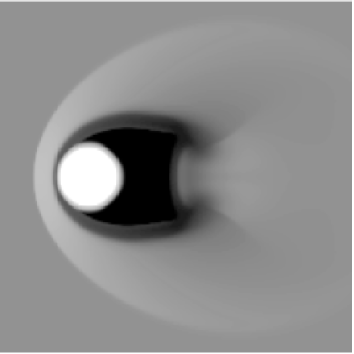
Figure 2: In this figure we show the temperature profile (in Kelvin) of the 30 000-year old PN shown in panel (f) of figure 1 on the same slice through the numerical domain.

Figure 2 shows the temperature distribution of the PN shown in panel (f) of Figure 1, 30 000 years into the PN phase. Given our calculation that the Stromgren sphere extends beyond the simulation domain, we assume that everything which is at 10⁴ K or lower is photo-ionised and that everything which has a temperature greater than $1.5\times 10^{4}$ K is collisionally ionised. Thus the material at the head of the bow shock appears to be collisionally ionised. Looking at the tail, the material is cooler and thus may be photo-ionised if the central star is still bright enough. This is the general case for the rest of our simulations where collisional ionisation of material can be inferred at the head of the bow shock with photo-heating/ionisation of the material stripped into the tail.

We define the previous phase where the PN was inside the AGB wind bubble as the first stage of PN–ISM interaction. The second stage would begin with the first indication of ISM interaction when the PN brightens in the direction of motion. This second stage will be responsible for rebrightening of ancient PNe and including this effect in the projection of current PN Galactic distributions may address the very long visible life time of PNe implied by recent studies (Moe & De Marco, 2006; Zijlstra & Pottasch, 1991).

The ISM interaction is clearly important even at these low speeds, as it shapes the AGB wind long before the PN phase. The AGB wind forms a bow shock upstream of the central star with tails stretching downstream. The PN does not interact with the AGB wind bow shock until it has expanded enough to reach the bow shock, typically after 25–30 000 years. At that point, the enhanced density and temperature of the material in the region of interaction suggests strengthening of the emission from that area: rebrightening. The parameter values in this case are comparable to those used by VGM and we have found similar effects on the PN formed, supporting our triple-wind model and conclusions.

4.2 Case B

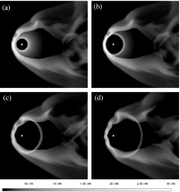
Figure 3: The results of case B: the panels show the gas density during the post–AGB phase. In panel (a), the simulation is 5 000 years into this phase, in panel (b) 10 000 years, in panel (c) 20 000 years and in panel (d) 30 000 years. The position of the central star is marked by an asterisk. The colour scaling is logarithmic and the density is scaled in units of $10^{-6}\ \mathrm{M_{\odot}\,pc}^{-3}$ where $2.5\times 10^{6}$ is equivalent to $n_{\rm H}$ = 100 cm^-3.

In Figure 3 we show the results of case B during the post–AGB phase. We do not show the AGB phase as the structure formed during this phase is clear in panel (a), where the PN has been expanding for 5000 years into the AGB wind bubble behind the bow shock. The central star is now moving at 50 $\mathrm{km\,s}^{-1}$, an average $v_{\rm ISM}$ for a PN-forming star. A bow shock has formed ahead of the central star during the AGB phase and stabilised at the point of ram pressure balance 0.25 pc ahead of the central star. This is a much smaller structure than in case A due to the increased ram pressure of the ISM. Further, the bow shock in this case is not smooth; instead there are indications of turbulent motion which can be seen originating in the AGB phase as instabilities at the head of the bow shock and moving back down the tail over tens of thousands of years. Note that the region between the forward shock and contact discontinuity is compressed upstream compared to the previous case. An investigation of the temperatures in this region shows that the material is far hotter at $\sim 30\,000$ K than in the previous case, in agreement with strong shock predictions, and therefore stronger radiative cooling can be inferred to be the cause of the forward shock compression. The PN is still inside the bubble of undisturbed AGB wind material and as yet unaffected by the ISM.

In panel (b), 10 000 years into the PN phase, the PN has reached the second stage of PN–ISM interaction whereby the PN still appears circular but is now rebrightened at the interaction with the AGB wind bow shock. The PN is also rapidly entering a third stage where the geometric centre of the nebula, defined as the centre of the circular/elliptical shape on the sky, is moving away from the central star.

After 20 000 years of PN evolution, the PN–ISM interaction has distorted the circular shape of the nebula as shown in panel (c). The central star appears displaced by a quarter of the diameter upstream of the geometric centre. The highest density and temperature regions have now moved around the bow shock to the point where the tail stretches away from the PN shell. These regions can be interpreted as areas where the nebular shell and ISM have driven the AGB wind material away from the head of the bow shock towards the tails. It is worth noting that at this time estimates of the nebular age via its observational dynamics (i.e. gas expansion velocity) would underestimate its true age.

In panel (d), 30 000 years into the PN phase, the PN has further departed from circular symmetry on the sky. The regions of highest density and temperature are towards the head of the fast wind bow shock which is now forming ahead of the star against the oncoming ISM. The nebular shell is still progressing downstream though the undisturbed AGB wind bubble and causing the geometric centre of the nebula to deviate downstream. This stage of significant deceleration of the upstream shell was considered by Soker et al. (1991).

At this typical $v_{\rm ISM}$, PN–ISM interaction has strongly affected the evolution of the PN. Rebrightening via interaction has occured at a much younger age of only a few thousand years and the shape of the PN has deviated strongly from circularity on the sky. One sided brightening and/or deviations from circular symmetry combined with an off-geometric-centre central star are clearly strong indicators of PN–ISM interaction. Further, these indicators are not limited to ancient or diffuse PNe. Such an interaction at this average speed would indicate many PNe should display some characteristics of ISM interaction during their later life.

4.3 Case C

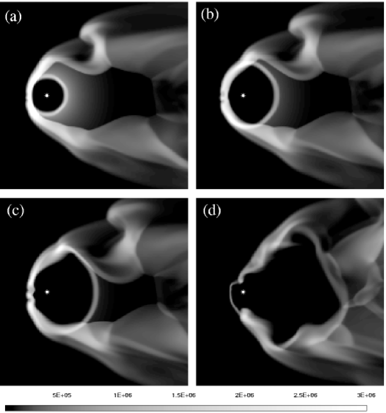
Figure 4: The results of case C: the panels show the gas density during the post–AGB phase. In panel (a), the simulation is 5000 years into this phase, in panel (b) 10 000 years, in panel (c) 15 000 years and in panel (d) 30 000 years. The position of the central star is marked by an asterisk. The colour scaling is logarithmic and the density is scaled in units of $10^{-6}\ \mathrm{M_{\odot}\,pc}^{-3}$ where $2.5\times 10^{6}$ is equivalent to $n_{\rm H}$ = 100 cm^-3.

In Figure 4, we show the results of case C during the post–AGB phase. In panel (a), 5000 years into this phase, the PN already has passed through the first stage of interaction and the large higher density region on the upstream side of the PN indicates it is now some way into the second stage. The stabilisation of the bow shock a shorter distance of 0.18-pc upstream is responsible for this earlier interaction. Note that with $v_{\rm ISM}$ = 75 $\mathrm{km\,s}^{-1}$ the bow shock is now seriously disrupted and instabilities noted in the previous case are now forming cool, high-density spiralling vortices moving down the tail. The origin of these vortices as vortex-shedding instabilities at the head of the bow shock and their effect on the local ISM are discussed elsewhere (Wareing, Zijlstra & O’Brien, 2007). We find the vortices will affect almost all bow shock structures and PNe will interact with them at some point during their evolution. A higher speed case carried out by VGM also revealed similar structures forming in the AGB wind bow shock (Szentgyorgyi et al., 2003).

In panel (b), the upstream portion of the nebular shell has been significantly decelerated causing the geometric centre of the nebula to shift downstream. At this stage, 10 000 years into the post–AGB phase, the regions of highest density and temperature have again moved round the bow shock and the PN is in the third stage of PN–ISM interaction.

In the third panel, 15 000 years into the post–AGB phase, the object is still recognisable as a PN, although the regions of highest density are in the tail of the bow shock. Finally, after 30 000 years of post–AGB evolution, the densest regions of the PN are indicative of the structure of the tail of the bow shock, including the effect of the vortices moving downstream. The thin fast wind bow shock is clear ahead of the PN-forming star, although the star is no longer anywhere near the centre of the object. This would be an ancient and probably very faint PN, but the PN–ISM interaction would still cause many parts of it to rebrighten.

In summary, the PN–ISM interaction is becoming more important at higher $v_{\rm ISM}$: the bow shock is closer to the star causing the PN to move through the stages of interaction more quickly. PN–ISM interaction would be apparent at a much earlier age even at this relatively average $v_{\rm ISM}$ of 75 $\mathrm{km\,s}^{-1}$.

4.4 Case D

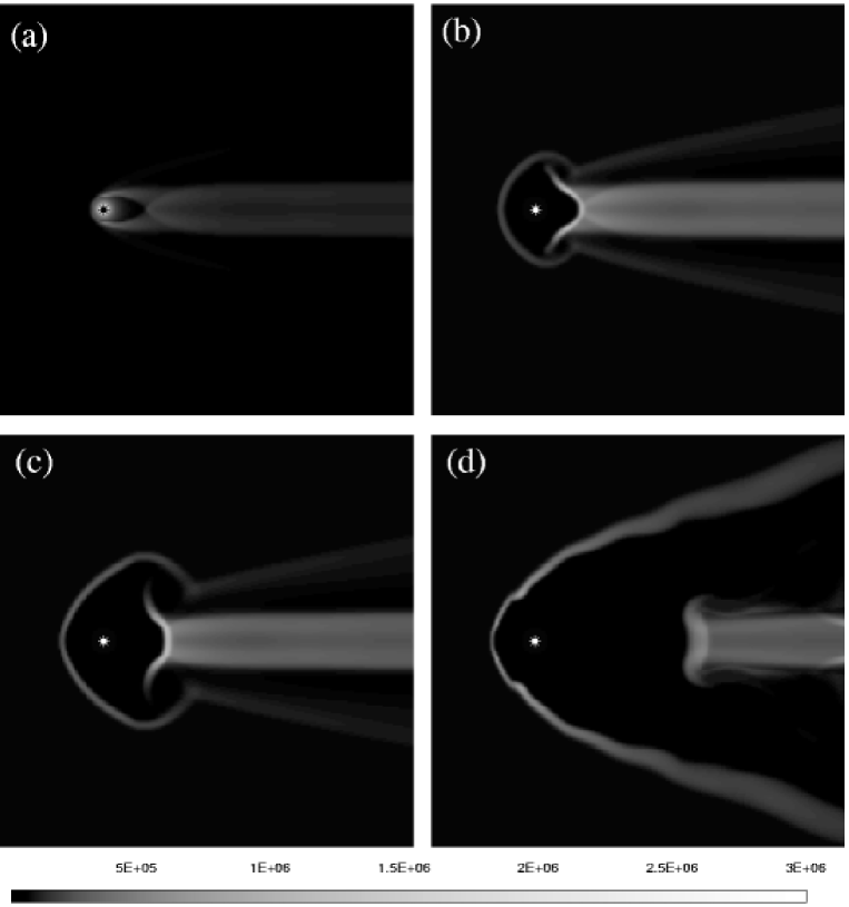
Figure 5: The results of case D: the panels show the gas density during the post–AGB phase. In panel (a), the simulation at the end of the AGB phase, in panel (b) 1000 years into the post–AGB phase, in panel (c) 2000 years and in panel (d) 10 000 years. The position of the central star is marked by an asterisk. The colour scaling is logarithmic and the density is scaled in units of $10^{-6}\ \mathrm{M_{\odot}\,pc}^{-3}$ where $2.5\times 10^{6}$ is equivalent to $n_{\rm H}$ = 100 cm^-3.

In Figure 5 we show the results of case D, where the central star has $v_{\rm ISM}$ = 100 $\mathrm{km\,s}^{-1}$. A narrow confined bow shock has formed ahead of the star, with a tail stretching far downstream, as shown in panel (a), by the end of the AGB phase. This central star could be considered much like a speeding bullet and the high $v_{\rm ISM}$ and high ISM density combined with the low mass-loss rate of the slow wind has resulted in a much more confined bow shock. The ISM has exerted a naturally stronger shaping influence due to greater ram pressure. Any instabilities at the head of the bow shock are either smoothed out by the oncoming ISM or flow out of the simulation before they have time to fully form.

In panel (b), 1000 years into the PN phase, the PN has very rapidly interacted with the bow shock and formed a fast wind bow shock further ahead of the central star, which can also be understood in terms of a ram pressure balance. Interestingly, the highest densities are in the region of the nebular shell which is moving downstream. In contrast to earlier cases, this portion of the shell is now closest to the star. It has rapidly moved through the small bubble of undisturbed AGB wind material and is now interacting with the more dense shocked AGB wind material in the tail. In panel (c), after 2000 years, this effect is even more apparent. Over the course of the next few thousand years, the tail of the wide fast wind bow shock grows downstream and the remaining part of the nebular shell continues to move away from the central star through the tail of older shocked AGB wind material.

The PN formed in this case is very different to many others and characteristic of small and confined bow shocks throughout our simulations. How observable the fast wind bow shock would be remains an open question as whilst it is hot, it is also of low density. The PN in this case has rapidly moved through the first three stages of PN–ISM interaction. We interpret the stage where the fast wind bow shock is forming and the remains of the nebular shell are fading whilst moving downstream as the fourth and final stage of PN–ISM interaction. During this stage, it is difficult to recognize the object, which would still be young enough to be observable, as a PN.

4.5 Case E

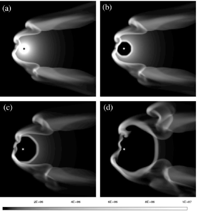
Figure 6: The results of case E: the panels show the gas density during the post–AGB phase. In panel (a), the simulation at the end of the AGB phase and the beginning of the post–AGB phase, in panel (b) 2000 years into the post–AGB phase, in panel (c) 4000 years and in panel (d) 10 000 years. The position of the central star is marked by an asterisk. The colour scaling is logarithmic and the density is scaled in units of $10^{-6}\ \mathrm{M_{\odot}\,pc}^{-3}$ where $5\times 10^{6}$ is equivalent to $n_{\rm H}$ = 200 cm^-3.

The final case under discussion in this paper is case E, shown in Figure 6. In this case the central star has a high $v_{\rm ISM}$ of 125 $\mathrm{km\,s}^{-1}$, a high ISM density and a high slow wind mass-loss rate. The bow shock structure is comparatively large because of the high mass-loss rate. Instabilities in the bow shock have caused multiple vortices to be shed downstream with an ensuing complex bow shock structure, as shown in panel (a) at the end of the AGB phase. The PN–ISM interaction is almost immediately apparent and after 2000 years, as shown in panel (b), the PN is mid-way through the second stage of interaction. The deceleration of the PN shell caused by the bow shock will soon cause the geometric centre to shift downstream and the PN to enter the third stage of interaction. Observing a PN with a high-velocity central star and a faint completion of the nebular ring moving downstream would indicate a young rather than old PN, even though the PN–ISM interaction is strongly apparent. In panel (c), 4000 years into the post–AGB phase, the densest regions of the PN have moved away from the head of the bow shock. The structure of the bow shock at the end of the AGB phase is having a very strong effect on the appearance of the PN – particularly the fact that the bow shock had fallen back towards the central star having just shed a vortex-causing instability downstream. In later stages (e.g. after 10 000 years shown in panel (d)) the vortices have become even more important for the evolution of the PN and are the regions of highest density. The object will eventually fade and look even less like a PN; faint objects serendipitiously discovered as part of Galactic surveys, e.g. IPHAS (Drew et al., 2005), may closely resemble this PN whilst not be classified as such. Eventually, after the central star has turned off and there is no longer a wind supporting the bow shock, the nebula would be rapidly blown downstream and the central star would move outside its nebula.

5 Discussion

5.1 The four stages of interaction

How a PN will interact with the ISM is set during the AGB phase and VGM was the first to highlight this important point. We have identified four stages of interaction which we call WZO 1–4. There is a phase of evolution where the PN is expanding within the bubble of undisturbed AGB wind material and this we define as the first stage of PN–ISM interaction, WZO 1. During this stage, a PN would be unaffected by the ISM interaction which is radially further from the central star. We suggest it would be possible during this stage to observe a faint arc around the PN, which would be the AGB wind bow shock. In the case of a slow-moving star with a large bow shock, this stage can last for the entire lifetime of the PN and it is unlikely a PN–ISM interaction will ever be observed. However, if the central star is moving even at average speed, the PN–ISM interaction can become rapidly apparent, in some of our simulations after only a thousand years. We show this stage in Figure 7(a).

The characteristic of stage 1 is a shell of swept-up ISM, up to a few pc away. This has been called a ’wall’ (Zijlstra & Weinberger, 2002). On sky images, this may also show up an area of reduced emission around the PN, ending at the wall. Evidence for such cavities has been presented by Evans et al. (2002) and Weinberger (2003).

Figure 7: A simple illustration of the appearance of a PN during the four stages of PN–ISM interaction discussed in section 5.1. The direction of motion is to the left and thicker lines indicate the brightest regions. Panel (a) illustrates stage WZO 1, (b) stage WZO 2), (c) stage WZO 3 and (d) stage WZO 4. The position of letters (a), (b), (c) and (d) indicate the position of the central star at each stage.

Stage WZO 2 is entered when the PN has expanded far enough to interact with the bow shock formed during the AGB phase of evolution. As the PN shock merges with the AGB wind bow shock, driving another shock through it, the density and temperature of the material increase accordingly and strengthen the emission from this area. This is shown in Figure 7(b). If $v_{\rm ISM}$ is predominantly in the plane of the sky, we would observe part of the nebular shell brighter than the rest. If, however, $v_{\rm ISM}$ is almost all along the line of sight to the PN, emision from the whole ring structure would strengthen and it would be difficult to identify this PN as undergoing a PN–ISM interaction until later in its evolution when distortions of the PN shell may reveal its true nature. This stage is relatively short lived and can be as short as a thousand years or so in our simulations with the largest $v_{\rm ISM}$. During this stage the whole PN continues to appear circular on the sky, but as the central star moves away from the geometric centre of the nebula, caused by the deceleration of the nebular shell in the direction of motion, the PN enters the third stage of PN–ISM interaction.

The third stage of interaction, WZO 3, is defined by the geometric centre of the nebula moving downstream away from the central star as shown in Figure 7(c). The shift of the geometric centre due to the deceleration of the PN shell in the direction of motion is guaranteed to occur and provides a measurable effect of this interaction. During this stage, and beginning during the second stage, it is difficult to estimate the age of the PN from its apparent diameter on the sky. The AGB wind–ISM interaction has coccooned the PN inside the AGB wind bow shock and this considerably inhibits the expansion of the PN shell during stages two and three. Identification of the arc of nebular shell moving downstream yet still inside the AGB wind bubble and the central star would provide an estimate of the radius of the PN if it had not been inhibited by the PN–ISM interaction. This radial distance could be used to dynamically estimate the age of the PN. Interestingly, our simulations suggest that a secondary effect during this stage is that the regions of highest density and temperature move away from the head of the bow shock. This can be understood as the oncoming ISM sweeping the shocked PN material from the second stage towards the tail of the nebula. This third stage can be open-ended and only in the higher $v_{\rm ISM}$ cases is the PN affected enough by the interaction to become completely unfamiliar and enter the fourth stage of interaction before it fades away. Even in the highest velocity cases, the third stage lasts at least 10 000 years. It is possible that in the most extreme cases, the PN shell will continue to appear circular as the nebula is swept downstream of the central star. Sh 2-68 is an example of a nebula where the central star is thought to have deserted its PN (Kerber, 2002).

In the fourth and final stage of PN–ISM interaction, WZO 4, the PN no longer appears circular. The fast wind has formed a bow shock ahead of the star and the little remaining AGB wind material in the vicinity of the star is being swept downstream with turbulent areas of high density and temperature as shown in Figure 7(d). At this time, the observable structure may not be identified as a PN. Further, the central star appears to have long since left these regions. Many objects such as this may exist and are probably not classified as PNe, affecting estimates of the Galactic distribution of PNe. Deep surveys in particular will be abe to uncover these objects.

Our four stages of the interaction are summarised in Table 2. The first two stages are similar to the stages of evolution suggested by Borkowski et al. (1990) from their observations of ancient PNe, although we find they can occur earlier in the PN evolution than considered in that work, due to the pre-shaping during the AGB.

Table 2: The four stages of PN–ISM interaction and their observable effects, as discussed in section 5.1

stage	observable effects
WZO 1	PN as yet unaffected; faint bow shock may be observable.
WZO 2	Brightening of PN shell in direction of motion.
WZO 3	Geometric centre shifts away from central star,
WZO 4	PN completely disrupted, central star is outside the PN.

Central stars of PNe which show evidence of interaction should have a proper motion consistent with the observed distortions across the plane of the sky if the nebula is close enough and the central star is moving fast enough in the right direction to have an appreciable angular motion over time. Borkowski et al. (1990) performed an investigation of PNe with known large angular motion and revealed many show signs of being in WZO Stage 2.

The largest value of proper motion of a central star measured via ground-based observations is $53.2\pm 5.5$ mas yr^-1. This is the proper motion of the central star of Sh 2-68 Kerber (2002). The measurement has provided direct confirmation of the process of the central star being displaced from the geometric centre of the nebula.

5.2 Missing mass

The interaction with the ISM considerably alters the amount of mass within the observed nebula: the ram-pressure stripping of material downstream during the AGB phase removes mass from the circumstellar region. Our simulations show that up to 90 per cent of the mass ejected from the star during the AGB phase can be left downstream forming the tail behind the nebula. This effect may provide a solution to the missing mass problem in PNe whereby only a small fraction of the mass ejected during the AGB phase is observationally inferred to be present during the post–AGB phase. Stellar evolution calculations predict that stars with initial masses in the range of 1–5 M_⊙ will end as PN nuclei with masses around 0.6 M_⊙. Most of the mass is lost on the AGB phase and should be easily observable as ionized mass during the PN stage. However, observations of Galactic PNe reveal on average only 0.2 M_⊙ of ionized gas. As the interaction progresses, the mass in the PN shell is increased during merger with the AGB wind bow shock, but this effect is minimal when compared to the mass left downstream. At higher speeds, the stripping effect is greater and more mass is lost downstream. Our simulations clearly support VGM’s conclusion that PN–ISM interaction at low speeds can provide an explanation of the missing mass phenomenon. Further, we show that this effect is even more pronounced at high speed.

Recent observations of the Mira system containg the AGB star Mira A have revealed a comet-like tail of material stretching 4 pc North away from the system (assuming a distance of 107 pc) and an arc-like structure in the South (Martin et al., 2007). Martin et al go on to comment that the space velocity of 130 $\mathrm{km\,s}^{-1}$ is in a direction consistent with the comet-like tail being a ram-pressure-stripped tail of material behind a bow shock ahead of the system, thereby confirming our postulation of tails of ram-pressure-stripped material behind AGB stars.

5.3 Limitations of the model

In reality, it is reasonable to expect the AGB wind to show an increasing mass-loss rate with time, whilst the post–AGB wind may increase in velocity over time. We have shown that our current assumptions are sufficient to reproduce basic nebular structure and leave detailed temporal modelling to a future publication.

In our models, we have not considered the intrinsic structure of the PN; as initially discussed, PN display many asymmetric shapes which cannot be explained in the context of this model. The inclusion of time-variant AGB and post–AGB wind parameters, asymmetric winds and/or magnetic fields may address this, but this is beyond this publication.

In contrast to the studies of Dgani & Soker (1994) and Dgani & Soker (1998), we have observed no fragmentation in our model above 100 $\mathrm{km\,s}^{-1}$. In an effort to understand whether grid resolution affects fragmentation, we have run a high resolution simulation on the head of the bow shock with effectively 8 times higher resolution and found no evidence of fragmentation. This disagreement could be attributed to the simulations being of too low resolution to allow instabilities to fragment the bow shock in such a way as theoretically predicted. Soker et al. (1991) did not consider evolution on the AGB which alters the structures considerably. Our simulations have not included the effect of magnetic field, neither as a scalar pressure nor a vector field. Magnetic fields, if inclined to the direction of relative motion, break the cylindrical symmetry of the interaction process which can affect these instabilities and lead to the formation of elongated structures. Huggins & Manley (2005) extends the suggestion that filaments observed in PNe may be signatures of an underlying magnetic field. We have demonstrated that magnetic fields are not necessary to explain asymmetries observed in slow-moving PNe. It is possible that the inclusion of a gravitational field in the hydrodynamic method may fragment the bow shocks but this is also beyond the scope of this work. Further, an inhomogeneous ISM could alter the structure of the bow shock.

In our simulations, we see instabilities forming at the head of the AGB wind bow shock causing vortex shedding downstream. When the PN shell expands far enough to interact with these vortices, typically during stage 3 or 4, it is affected and the PN shell would be distorted and brightened accordingly. We have discussed the importance of these vortices for the local ISM elsewhere (Wareing, Zijlstra & O’Brien, 2007). Inhomogeneities in the ISM could be expected to seed more instabilities for vortices.

Finally, we note that observability of such objects is dependent on the extent of the photoionisation and on excited ionisation lines.

6 Comparisons to observed PNe

6.1 Relevance for Galactic Disk PNe

We have briefly examined the IAC Morphological Catalog of Northern Galactic Planetary Nebulae (Manchado et al., 1996) and list in Table 3 the PNe which we suggest are interacting with the ISM, the stage of their PN–ISM interaction and their brief interaction characteristics.

Table 3: Nebulae displaying characteristics of ISM interaction from the IAC Morpohological Catalog of Northern Galactic Planetary nebulae (Manchado et al., 1996) discussed in Section 6.1

Name	Stage of	Charecteristics
	interaction
A 13	WZO 2	bow shock/PN interaction to the West
A 16	WZO 2	bow shock/PN interaction to the South-East
A 52	WZO 2	bow shock/PN interaction to the North-East
A 58	WZO 2	brightened on the Western side; may be a bow shock interaction
A 59	WZO 2	bow shock/PN interaction to the North
A 86	WZO 2	bow shock/PN interaction to the North-East
Ba 1	WZO 1	faint bow shock structure outside PN to the North-West
DeHt 2	WZO 1	faint bow shock structure outside PN to the North
DeHt 4	WZO 2	bow shock/PN interaction to the West
EGB 4	WZO 3/4	narrow, confined (fast wind?) bow shock to the South
He 2-428	WZO 2	bow shock/PN interaction to the South
IC 4593	WZO 1	faint bow shock structure outside PN to the North-West
Jn 1	WZO 3	bow shock/PN interaction with emission shifted downstream
K 2-2	WZO 3/4	structure may be a bow shock remnant
K 4-5	WZO 3/4	structure may be remnant of a bow shock blown downstream
M 2-2	WZO 2	bow shock/PN interaction to the South
M 2-40	WZO 1	faint bow shock structure outside PN to the East
M 2-44	WZO 1	faint bow shock structure outside PN to the South-West
NGC 6765	WZO 1	faint bow shock structure outside PN to the West
NGC 6853	WZO 1	faint bow shock structure outside PN to the North-West
NGC 6891	WZO 1	faint bow shock structure outside PN to the South-West
S 22	WZO 2	bow shock/PN interaction to the South-East
Sd 1	WZO 2	bow shock/PN interaction to the North

Of the approximately 130 well-resolved nebulae in the catalogue, if we assume a random distribution of angles between $v_{\rm ISM}$ and the line of sight then approximately 15–20 per cent of the nebulae will have their motion predominantly in the plane of the sky. PN–ISM interaction is clear in cases where $v_{\rm ISM}$ is in the plane of the sky and our brief inspection of the catalogue has revealed 20 per cent show characteristics of PN–ISM interaction. The correlation between these statistics supports our finding that interaction is common, particularly amongst large and/or evolved PNe. A further study of our selected PNe may reveal angular motions of the central stars, which should be in the direction of the ISM interaction.

Considering the list of PNe given by Borkowski et al. (1990), we find that all of them are in the WZO 1 or WZO 2 stages of PN–ISM interaction.

6.2 Relevance for Galactic Bulge PNe

Galactic Bulge PNe have central stars with higher typical $v_{\rm ISM}$. Our simulations have shown that simulations with higher typical $v_{\rm ISM}$ are generally smaller and show signs of strong interaction at an earlier age, thus we would expect Galactic Bulge PNe to have such characteristics.

6.3 Relevance for PNe in globular clusters

Three PNe are known in globular clusters. The PN in M15 (K648) shows a strongly edge-brightened structure, reminiscent of a WZO 2 interaction (Alves et al., 2000). The PN in M22 is known to be peculiar, strong in [O III] but absent in H$\alpha$: it is worth investigating the possible effect of shock-excitation on its spectrum. Its structure shows a clear bow shock (Borkowski et al., 1993), with the star close to the parabolic arc. This can be identified with a type WZO 2 interaction. The tail is not seen.

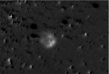
Figure 8: VLT FORS1 image in [O III] of the PN in NGC 6441. Continuum has been subtracted. The edge brightening is indicative a PN–ISM shock.

The final confirmed globular cluster PN (Jacoby et al., 1997) is in the cluster NGC 6441. No previous high-resolution images have been published. We obtained an image taken with the VLT in [O III], background subtracted, courtesy of M. van Haas and L. Kaper. The image is shown in Fig. 8: it shows a clear edge brightening, with the brightest region possibly split from the head of the bow shock. This is indicative for an early type WZO 3 interaction. We conclude that all three globular cluster PNe are dominated by ISM interaction.

As globular clusters have been stripped of their interstellar gas and are moving at high velocities (up to 200 $\mathrm{km\,s}^{-1}$) through the Galactic halo, we would expect to see severe effects for these short-lived objects including rapid brightening via interaction and destruction.

7 Conclusions

Observationally, the presence of asymmetries in the haloes of PNe has been found to be a relatively common feature (Tweedy & Kwitter, 1996; Guerrero et al., 1998). These asymmetries can be partially if not wholly attributed to interaction with the ISM. The high rate of asymmetries can now be explained when the evolution through the AGB phase of the central star is considered. The simulations in this work show that interaction is present at all evolutionary stages for all $v_{\rm ISM}$.

Our comprehensive simulations have reinforced the result of VGM that PN–ISM interaction is set during the AGB phase and affects central stars with typical $v_{\rm ISM}$, not just those with extreme velocities. We have developed a model which results in four stages of ISM interaction and inspections of PNe support this four stage interpretation.

PNe have been found to evolve more quickly through these stages the faster they move through the ISM. They have also been found to be smaller for greater $v_{\rm ISM}$. Much of their mass ejected during the AGB phase has been stripped downstream into the tail, providing a possible explanation of the missing mass problem observed in PNe, with evidence for such a tail found by Martin et al. (2007). The average speed results of the model appear very similar to the recently discovered bow shock surrounding the Dumbbell Nebula which has an average $v_{\rm ISM}$ (Meaburn et al., 2005) further supporting our model.

Our conclusions are in agreement with VGM using similar models. We have extended the study of the PN–ISM interaction including the AGB phase to three dimensions and higher $v_{\rm ISM}$ where they were previously limited to two dimensions and low $v_{\rm ISM}$.

PNe which show signs of ISM interaction are not necessarily ancient, nor require a high $v_{\rm ISM}$ or magnetic fields. Interaction can become apparent at a young age via several methods and central stars with an average $v_{\rm ISM}$ can show evidence of interaction in their nebulae, as commonly observed, and be displaced from the geometric centre of their nebulae. None of the simulations have required a magnetic field to produce commonly observed effects, although the fragmentation of the bow shock in PNe as Sh 2-188 awaits a fuller treatment of this interaction at higher resolutions involving inhomogeneous ISM and gravitational and magnetic field modelling to reasonably test the fragmentation theories of interacting PNe.

Appendix A Appendix 1

In figures 1–8, we show slices of the simulation domain through the position of the central star, parallel to the direction of motion at the end of the AGB phase of evolution. Each figure shows the set of simulations at a particular $v_{\rm ISM}$. In the accompanying tables 1–8, we list the parameter values for each simulation.

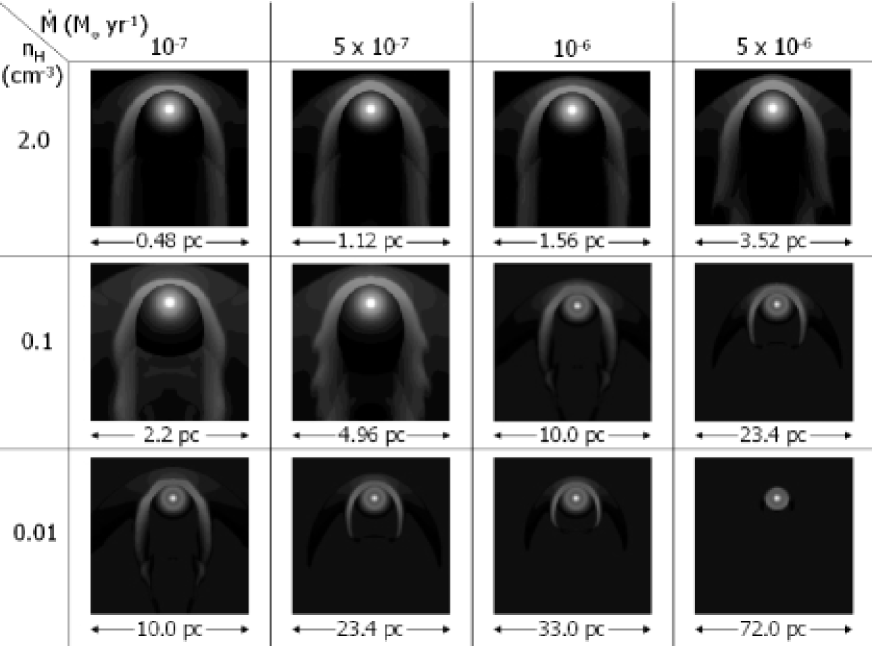
Figure 9: Snapshots at the end of the AGB phase of evolution for $v_{\rm ISM}$ = 25 $\mathrm{km\,s}^{-1}$. mass-loss rate increases from left to right, ISM density decreases from top to bottom. Full details of each simulation can be found in table 4.

Table 4: Input parameters for the PN–ISM simulations in figure 9: column a) gives the mass-loss rate in the slow wind; column b) the density of the surronding ISM in $n_{\rm H}\,\rm cm^{-3}$; column c) the relative velocity of the central star; column d) the grid dimension along one side.

a)	b)	c)	d)
$\dot{M}_{\rm sw}$	$\rho_{\rm ISM}$	$v_{\rm ISM}$	Grid
(M⊙ yr-1)	$n_{\rm H}$(cm-3)	($\mathrm{km\,s}^{-1}$)	(pc)
$10^{-7}$	2	25	0.48
$5\times 10^{-7}$	2	25	1.12
$10^{-6}$	2	25	1.56
$5\times 10^{-6}$	2	25	3.52
$10^{-7}$	0.1	25	2.2
$5\times 10^{-7}$	0.1	25	4.96
$10^{-6}$	0.1	25	10.0
$5\times 10^{-6}$	0.1	25	23.4
$10^{-7}$	0.01	25	10.0
$5\times 10^{-7}$	0.01	25	23.4	case A
$10^{-6}$	0.01	25	33.0
$5\times 10^{-6}$	0.01	25	72.0

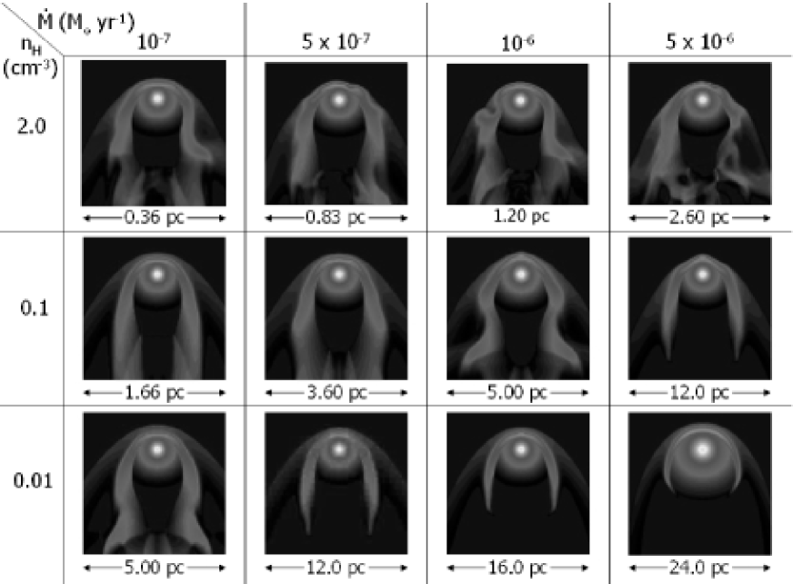
Figure 10: Snapshots at the end of the AGB phase of evolution for $v_{\rm ISM}$ = 50 $\mathrm{km\,s}^{-1}$. mass-loss rate increases from left to right, ISM density decreases from top to bottom. Full details of each simulation can be found in table 5.

Table 5: Input parameters for the PN–ISM simulations in figure 10: column a) gives the mass-loss rate in the slow wind; column b) the density of the surronding ISM in $n_{\rm H}\,\rm cm^{-3}$; column c) the relative velocity of the central star; column d) the grid dimension along one side.

a)	b)	c)	d)
$\dot{M}_{\rm sw}$	$\rho_{\rm ISM}$	$v_{\rm ISM}$	Grid
(M⊙ yr-1)	$n_{\rm H}$(cm-3)	($\mathrm{km\,s}^{-1}$)	(pc)
$10^{-7}$	2	50	0.36
$5\times 10^{-7}$	2	50	0.83
$10^{-6}$	2	50	1.20
$5\times 10^{-6}$	2	50	2.60	case B
$10^{-7}$	0.1	50	1.66
$5\times 10^{-7}$	0.1	50	3.60
$10^{-6}$	0.1	50	5.0
$5\times 10^{-6}$	0.1	50	12.0
$10^{-7}$	0.01	50	5.0
$5\times 10^{-7}$	0.01	50	12.0
$10^{-6}$	0.01	50	16.0
$5\times 10^{-6}$	0.01	50	24.0

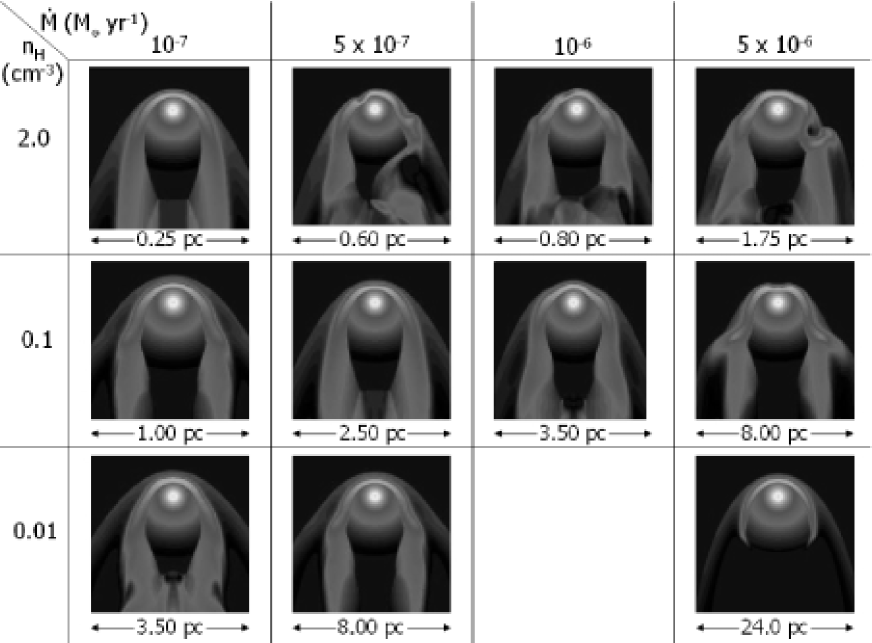
Figure 11: Snapshots at the end of the AGB phase of evolution for $v_{\rm ISM}$ = 75 $\mathrm{km\,s}^{-1}$. mass-loss rate increases from left to right, ISM density decreases from top to bottom. Full details of each simulation can be found in table 6. The ’missing’ simulation in the bottom row indicates the reduction in the mass-loss parameter range due to computational and time constraints.

Table 6: Input parameters for the PN–ISM simulations in figure 11: column a) gives the mass-loss rate in the slow wind; column b) the density of the surronding ISM in $n_{\rm H}\,\rm cm^{-3}$; column c) the relative velocity of the central star; column d) the grid dimension along one side.

a)	b)	c)	d)
$\dot{M}_{\rm sw}$	$\rho_{\rm ISM}$	$v_{\rm ISM}$	Grid
(M⊙ yr-1)	$n_{\rm H}$(cm-3)	($\mathrm{km\,s}^{-1}$)	(pc)
$10^{-7}$	2	75	0.25
$5\times 10^{-7}$	2	75	0.60
$10^{-6}$	2	75	0.80
$5\times 10^{-6}$	2	75	1.75	case C
$10^{-7}$	0.1	75	1.0
$5\times 10^{-7}$	0.1	75	2.50
$10^{-6}$	0.1	75	3.50
$5\times 10^{-6}$	0.1	75	8.0
$10^{-7}$	0.01	75	3.50
$5\times 10^{-7}$	0.01	75	8.0
$5\times 10^{-6}$	0.01	75	24.0

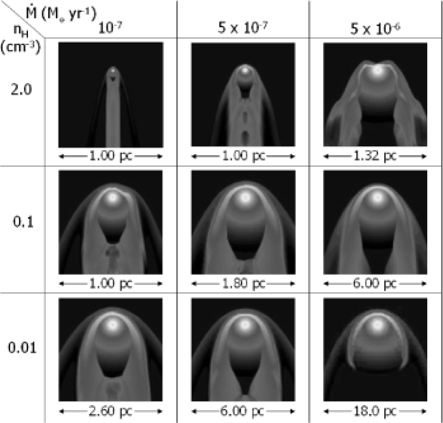
Figure 12: Snapshots at the end of the AGB phase of evolution for $v_{\rm ISM}$ = 100 $\mathrm{km\,s}^{-1}$. mass-loss rate increases from left to right, ISM density decreases from top to bottom. Full details of each simulation can be found in table 7.

Table 7: Input parameters for the PN–ISM simulations in figure 12: column a) gives the mass-loss rate in the slow wind; column b) the density of the surronding ISM in $n_{\rm H}\,\rm cm^{-3}$; column c) the relative velocity of the central star; column d) the grid dimension along one side.

a)	b)	c)	d)
$\dot{M}_{\rm sw}$	$\rho_{\rm ISM}$	$v_{\rm ISM}$	Grid
(M⊙ yr-1)	$n_{\rm H}$(cm-3)	($\mathrm{km\,s}^{-1}$)	(pc)
$10^{-7}$	2	100	2.0	case D
$5\times 10^{-7}$	2	100	2.0
$5\times 10^{-6}$	2	100	1.32
$10^{-7}$	0.1	100	1.0
$5\times 10^{-7}$	0.1	100	1.8
$5\times 10^{-6}$	0.1	100	6.0
$10^{-7}$	0.01	100	2.6
$5\times 10^{-7}$	0.01	100	6.0
$5\times 10^{-6}$	0.01	100	18.0

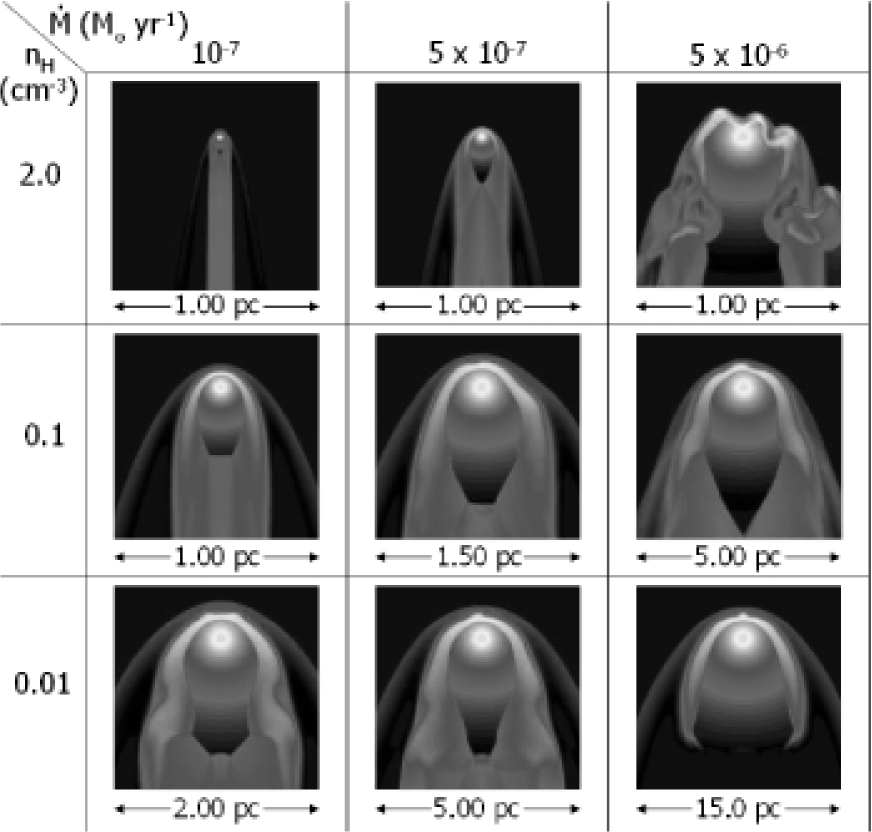
Figure 13: Snapshots at the end of the AGB phase of evolution for $v_{\rm ISM}$ = 125 $\mathrm{km\,s}^{-1}$. mass-loss rate increases from left to right, ISM density decreases from top to bottom. Full details of each simulation can be found in table 8.

Table 8: Input parameters for the PN–ISM simulations in figure 13: column a) gives the mass-loss rate in the slow wind; column b) the density of the surronding ISM in $n_{\rm H}\,\rm cm^{-3}$; column c) the relative velocity of the central star; column d) the grid dimension along one side.

a)	b)	c)	d)
$\dot{M}_{\rm sw}$	$\rho_{\rm ISM}$	$v_{\rm ISM}$	Grid
(M⊙ yr-1)	$n_{\rm H}$(cm-3)	($\mathrm{km\,s}^{-1}$)	(pc)
$10^{-7}$	2	125	1.0
$5\times 10^{-7}$	2	125	1.0
$5\times 10^{-6}$	2	125	1.0	case E
$10^{-7}$	0.1	125	1.0
$5\times 10^{-7}$	0.1	125	1.5
$5\times 10^{-6}$	0.1	125	5.0
$10^{-7}$	0.01	125	2.0
$5\times 10^{-7}$	0.01	125	5.0
$5\times 10^{-6}$	0.01	125	15.0

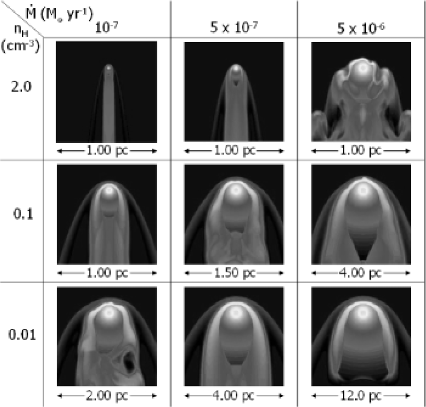
Figure 14: Snapshots at the end of the AGB phase of evolution for $v_{\rm ISM}$ = 150 $\mathrm{km\,s}^{-1}$. mass-loss rate increases from left to right, ISM density decreases from top to bottom. Full details of each simulation can be found in table 9.

Table 9: Input parameters for the PN–ISM simulations in figure 14: column a) gives the mass-loss rate in the slow wind; column b) the density of the surronding ISM in $n_{\rm H}\,\rm cm^{-3}$; column c) the relative velocity of the central star; column d) the grid dimension along one side.

a)	b)	c)	d)
$\dot{M}_{\rm sw}$	$\rho_{\rm ISM}$	$v_{\rm ISM}$	Grid
(M⊙ yr-1)	$n_{\rm H}$(cm-3)	($\mathrm{km\,s}^{-1}$)	(pc)
$10^{-7}$	2	150	1.0
$5\times 10^{-7}$	2	150	1.0
$5\times 10^{-6}$	2	150	1.0
$10^{-7}$	0.1	150	1.0
$5\times 10^{-7}$	0.1	150	1.5
$5\times 10^{-6}$	0.1	150	4.0
$10^{-7}$	0.01	150	2.0
$5\times 10^{-7}$	0.01	150	4.0
$5\times 10^{-6}$	0.01	150	12.0

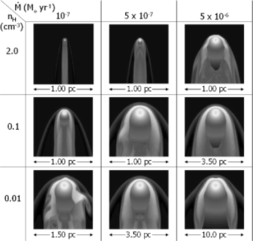
Figure 15: Snapshots at the end of the AGB phase of evolution for $v_{\rm ISM}$ = 175 $\mathrm{km\,s}^{-1}$. mass-loss rate increases from left to right, ISM density decreases from top to bottom. Full details of each simulation can be found in table 10.

Table 10: Input parameters for the PN–ISM simulations in figure 15: column a) gives the mass-loss rate in the slow wind; column b) the density of the surronding ISM in $n_{\rm H}\,\rm cm^{-3}$; column c) the relative velocity of the central star; column d) the grid dimension along one side.

a)	b)	c)	d)
$\dot{M}_{\rm sw}$	$\rho_{\rm ISM}$	$v_{\rm ISM}$	Grid
(M⊙ yr-1)	$n_{\rm H}$(cm-3)	($\mathrm{km\,s}^{-1}$)	(pc)
$10^{-7}$	2	175	1.0
$5\times 10^{-7}$	2	175	1.0
$5\times 10^{-6}$	2	175	1.0
$10^{-7}$	0.1	175	1.0
$5\times 10^{-7}$	0.1	175	1.0
$5\times 10^{-6}$	0.1	175	3.5
$10^{-7}$	0.01	175	1.5
$5\times 10^{-7}$	0.01	175	3.5
$5\times 10^{-6}$	0.01	175	10.0

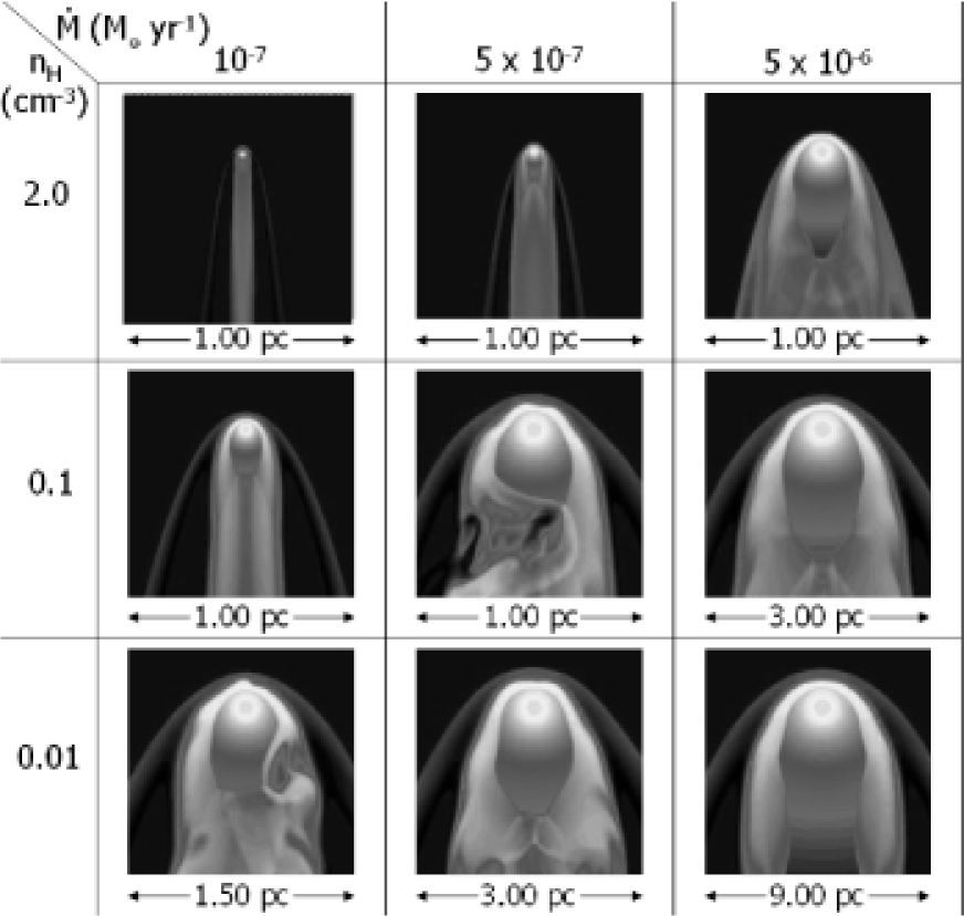
Figure 16: Snapshots at the end of the AGB phase of evolution for $v_{\rm ISM}$ = 200 $\mathrm{km\,s}^{-1}$. mass-loss rate increases from left to right, ISM density decreases from top to bottom. Full details of each simulation can be found in table 11.

Table 11: Input parameters for the PN–ISM simulations in figure 16: column a) gives the mass-loss rate in the slow wind; column b) the density of the surronding ISM in $n_{\rm H}\,\rm cm^{-3}$; column c) the relative velocity of the central star; column d) the grid dimension along one side.

a)	b)	c)	d)
$\dot{M}_{\rm sw}$	$\rho_{\rm ISM}$	$v_{\rm ISM}$	Grid
(M⊙ yr-1)	$n_{\rm H}$(cm-3)	($\mathrm{km\,s}^{-1}$)	(pc)
$10^{-7}$	2	200	1.0
$5\times 10^{-7}$	2	200	1.0
$5\times 10^{-6}$	2	200	1.0
$10^{-7}$	0.1	200	1.0
$5\times 10^{-7}$	0.1	200	1.0
$5\times 10^{-6}$	0.1	200	3.0
$10^{-7}$	0.01	200	1.5
$5\times 10^{-7}$	0.01	200	3.0
$5\times 10^{-6}$	0.01	200	9.0

References

- Alves et al. (2000) Alves D.R., Bond H.E., Livo M., 2000, AJ, 120, 2044
- Balick (1987) Balick B., 1987, AJ, 94, 671
- Binney & Merrifield (1998) Binney J., Merrifield M., 1998, in Galactic Astronomy (Princeton, NJ: Princeton University Press), Ch. 10
- Borkowski et al. (1990) Borkowski K.J., Sarazin C.L., Soker N., 1990, ApJ, 360, 173
- Borkowski et al. (1993) Borkowski K.J., Tsvetanov Z., Harrington J.P., 1993, ApJ, 402, L57
- Burton (1988) Burton W.B., 1988, in Galactic and Extragalactic Radio Astronomy, ed. K. Kellermann & G.L. Verschuur (New York: Springer), 295
- Dgani & Soker (1994) Dgani R., Soker N., 1994, ApJ, 434, 262
- Dgani & Soker (1998) Dgani R., Soker N., 1998, ApJ, 495, 337
- Drew et al. (2005) Drew J.E. et al., 2005, MNRAS, 362, 753
- Evans et al. (2002) Evans A. et al., 2002, MNRAS, 332, L35
- Falle (1991) Falle S.A.E.G., 1991, MNRAS, 250, 581
- Frank & Blackman (2004) Frank A., Blackman A.G., 2004, ApJ, 614, 737
- Guerrero et al. (1998) Guerrero M.A., Villaver E., Manchado A., 1998, ApJ, 507, 889
- Gurzadyan (1969) Gurzadyan G.A., 1969, Planetary Nebula (New York: Gordon & Breach), p.235
- Higgins et al. (1999) Higgins S.A., O’Brien T.J., Dunlop S.J., 1999, MNRAS, 309, 273
- Huggins & Manley (2005) Huggins P.J., Manley S.P., 2005, PASP, 177, 665
- Isaacmann (1979) Isaacmann R., 1979, A&A, 77, 327
- Jacoby et al. (1997) Jacoby G., Morse J.A., Fullton L.K., Kwitter K.B., Henry R.B.C., 1997, AJ, 114, 2611
- Kahn (1985) Kahn F.D., West K.A., 1984, MNRAS, 212, 837
- Kerber (2002) Kerber F., Guglielmetti F., Mignani R., Roth M., 2002, A&A, 381, L9
- Kwok (1982) Kwok S., 1982, AJ, 258, 280
- Lloyd et al. (1997) Lloyd H.M., O’Brien T.J., Bode M.F., 1997, MNRAS, 284, 137
- Manchado et al. (1996) Manchado A., Guerrero M.A., Stanghellini L., Serra–Ricart M., 1996, The IAC morphological catalog of northern Galactic planetary nebulae, Publisher: La Laguna, Spain: Instituto de Astrofisica de Canarias (IAC)
- Martin et al. (2007) Martin, D.C. et al. 2007, Nature, 448, 780
- Meaburn et al. (2005) Meaburn J. et al., 2005, Rev. Mex. AA, 41, 109
- Mitchell (2007) Mitchell D.L.M. 2007, PhD Thesis, Univ. of Manchester
- Moe & De Marco (2006) Moe M., De Marco O., 2006, ApJ, 650, 916
- Oort (1951) Oort J.H., 1951, Problems of Cosmical Aerodynamics (Dayton: Central Air Document Office)
- Porter et al. (1998) Porter J.M., O’Brien T.J., Bode M.F., 1998, MNRAS, 296, 943
- Raymond et al. (1976) Raymond J.C., Cox D.P., Smith B.W., 1976, ApJ, 204, 290
- Sanggak (1984) Sanggak S.G., 1984, AJ, 89, 702
- Skuljan et al. (1999) Skuljan J., Hearnshaw J.B., Cottrell P.L., 1999, MNRAS, 308, 731
- Smith (1976) Smith H., 1976, MNRAS, 175, 419
- Soker et al. (1991) Soker N., Borkowski K.J., Sarazin C.L., 1991, AJ, 102, 1381
- Soker (1996) Soker N., 1996, ApJ, 469, 734
- Szentgyorgyi et al. (2003) Szentgyorgyi A., Raymond J., Franco F., Villaver E., Lopez–Martin L. 2003, ApJ, 594, 874
- Tweedy & Kwitter (1996) Tweedy R.W, Kwitter K.B., 1996, ApJS, 107, 255
- Ueta et al. (2006) Ueta T., et al. 2006, ApJ, 648, L39
- Villaver et al. (2003) Villaver E., Garcia–Segura G., Manchado A., 2003, ApJ, 585, L53 (VGM)
- Wareing (2005) Wareing C.J. 2005, PhD thesis, Univ. of Manchester
- Wareing et al. (2006a) Wareing C.J., et al., 2006a, MNRAS, 366, 387
- Wareing et al. (2006b) Wareing C.J., et al., 2006b, MNRAS, 372, L63
- Wareing, Zijlstra & O’Brien (2007) Wareing C.J., Zijlstra A.A., O’Brien T.J., 2007, ApJ, 660, L129
- Weinberger (2003) Weinberger R., 2003, in: Planetary Nebulae: Their Evolution and Role in the Universe, Eds. Sun Kwok, Michael Dopita, and Ralph Sutherland. IAU Symp 209, p. 454
- Zijlstra & Pottasch (1991) Zijlstra A.A., Pottasch S.R., 1991, A&A, 243, 478
- Zijlstra & Weinberger (2002) Zijlstra A.A., Weinberger R., 2002, ApJ, 572, 1006