Thermal denaturation of fluctuating finite DNA chains:
the role of bending rigidity in bubble nucleation

Abstract

Statistical DNA models available in the literature are often effective models where the base-pair state only (unbroken or broken) is considered. Because of a decrease by a factor of 30 of the effective bending rigidity of a sequence of broken bonds, or bubble, compared to the double stranded state, the inclusion of the molecular conformational degrees of freedom in a more general mesoscopic model is needed. In this paper we do so by presenting a 1D Ising model, which describes the internal base pair states, coupled to a discrete worm like chain model describing the chain configurations [J. Palmeri, M. Manghi, and N. Destainville, Phys. Rev. Lett. 99, 088103 (2007)]. This coupled model is exactly solved using a transfer matrix technique that presents an analogy with the path integral treatment of a quantum two-state diatomic molecule. When the chain fluctuations are integrated out, the denaturation transition temperature and width emerge naturally as an explicit function of the model parameters of a well defined Hamiltonian, revealing that the transition is driven by the difference in bending (entropy dominated) free energy between bubble and double-stranded segments. The calculated melting curve (fraction of open base pairs) is in good agreement with the experimental melting profile of polydA-polydT and, by inserting the experimentally known bending rigidities, leads to physically reasonable values for the bare Ising model parameters. Among the thermodynamical quantities explicitly calculated within this model are the internal, structural, and mechanical features of the DNA molecule, such as bubble correlation length and two distinct chain persistence lengths. The predicted variation of the mean-square-radius as a function of temperature leads to a coherent novel explanation for the experimentally observed thermal viscosity transition. Finally, the influence of the DNA strand length is studied in detail, underlining the importance of finite size effects, even for DNA made of several thousand base pairs. Simple limiting formulæ, useful for analyzing experiments, are given for the fraction of broken base pairs, Ising and chain correlation functions, effective persistence lengths, and chain mean-square-radius, all as a function of temperature and DNA length.

I Introduction

The stability of double-stranded DNA (dsDNA) at physiological temperature is due to the self-assembly of its base pairs: self-assembly within a same strand via base-stacking interactions between neighboring bases; and self-assembly of both strands via hydrogen bonds between pairs of complementary bases. These interactions, however. are on the order of magnitude of a few $k_{B}T$ (thermal energy) SantaLucia98 ; pincet ; krueger and thermal fluctuations can lead, even at physiological temperature, to local and transitory unzipping of the double strand (see e.g. wartmont or the reviews gotoh ; lazurkin ). The cooperative opening of a sequence of consecutive base pairs leads to denaturation bubbles which are likely to play a role from a biological perspective, since they may participate in mechanisms such as replication, transcription or protein binding. For example, it has been proposed Kalosakas04 that transcription start and regulatory sites could be related to DNA regions which have a higher probability of promoting bubbles. Indeed, the energy needed to break an adenine-thymine (A-T) base pair $\sim 4k_{B}T$, connected by two hydrogen bonds, is smaller than the energy needed to break a guanine-cytosine (G-C) one $\sim 6k_{B}T$ (3 hydrogen bonds) SantaLucia98 ; pincet . At the same temperature, A-T rich sequences present a priori more bubbles than G-C rich ones, even though sequence effects on the occurrence of bubbles are more complex than a simple examination of local A-T base abundance SantaLucia98 ; Kalosakas04 . In addition to the sequence, the fraction of denaturation bubbles in vitro naturally depends on temperature, as well as on the ionic strength of the solution gotoh ; record . In particular, the melting temperature $T_{m}$, above which bubbles proliferate and the two strands completely separate, depends on both sequence and ionic strength. Another parameter that affects the melting temperature is the length of the double strand blake ; nelson . This is not a purely academic debate because short DNA strands (a few tens of base pairs) are involved in DNA chip experiments where the hybridization process is precisely affected by temperature in a way depending on strand length and sequence (see Fiche06 and references therein).

Although the intracellular unwinding of DNA is due to active and enzymatic processes by imposing unwinding torsional stresses benham , the thermally induced denaturation of purified DNA in solution has led to an intensive study of DNA thermal denaturation polscher ; lazurkin ; wartmont ; gotoh ; wartben . Mesoscopic models have been proposed to account for the thermodynamical properties of denaturation bubbles in DNA. The first models were Ising-like two-state models, where the base pairs can be open or closed (see wartmont ; gotoh and references therein). In the simple base-pair model, the Ising parameters are the base-pair chemical potential and the so-called cooperativity parameter, which accounts for the energetic cost of a domain wall. This type of one-dimensional Ising model is exactly soluble for homopolymers and for random sequences wartmont . More sophisticated effective Ising models, including the 10 kinds of base-pair doublets, lead to better agreement with experimental data gotoh . Poland and Scheraga polscher , following the work of Zimm zimm , included “loop entropy” in these models, i.e. the entropic cost of closing large loops formed by destacked single-stranded DNA (ssDNA) in bubbles polscher ; wartmont . This Poland-Scheraga model is at the core of the DNA melting simulator MELTSIM algorithm first developed by Blake et al. meltsim ; blake2 . The intra-loop and inter-loop self-avoidance corrects the loop statistics and refines the sharpness of the denaturation transition peliti ; carlon . To get a denaturation transition in these models, an effective temperature dependent Ising chemical potential must be inserted by hand. Recently, Peyrard et al. developed non-linear phonon models where the shape of the interaction potential between base pairs is more precisely taken into account (see peyrard ; dauxois ; hwa and the review peyrardreview ). By inserting estimated microscopic parameters, they have shown that their model can both lead to a denaturation transition, analogous to interface unbinding, and be useful for studying bubble dynamics. The predicted transition temperature is, however, very sensitive to the model parameter values, and if physically reasonable values are used dauxois ; gao ; jeon , $T_{m}$ appears to be much too high and the transition width much too large.

More generally, the theoretical study of DNA denaturation can in principle be tackled on a least four levels of investigation determined by the amount of detail included, going from (1) quantum ab initio approaches and (2) classical all atom molecular dynamical simulations amber , through (3) effective mesoscopic approaches coupling chain conformational and base-pair degrees of freedom orland , to (4) effective statistical models for base-pairs alone (wartmont ; polscher ; peyrardreview and references therein). In theory, it is possible to move up one step in this hierarchy by integrating out the subset of the degrees of freedom that do not appear at the higher level, giving rise to en effective free energy at each level of description. Our purpose here is to show, via a minimal model for DNA homopolymers, that if one starts at the third level and integrates out the chain degrees of freedom, one arrives at a physically coherent level (4) explanation for the DNA melting transition: a bending free energy driven denaturation transition emerges naturally due to the entropic lowering of the energetic barrier for bubble nucleation. Working at level (3) also has the added advantage of allowing access to the statistics of the chain degrees of freedom (effective persistence length, mean-square-radius, etc.), something that obviously is not possible at level (4).

To this end, we have recently proposed a model prl , which considers not only the internal coordinates in terms of Ising spin variables describing the open or closed states, but also external coordinates, the chain tangent vectors, which determine the chain configuration and depend sensitively on chain stiffness. Indeed, ssDNA is two orders of magnitude more flexible than dsDNA at normal salt concentration. We have shown that this difference in bending rigidity provides a novel explanation for the bubble mechanism formation. Further evidence for the importance of this bending heterogeneity include phenomena such as cyclization, loop formation, and packaging of DNA into nucleosomes Marko04 (where denaturation bubbles facilitate bending of the otherwise rigid polymer DNA in structures where it coils up with curvature radii down to 10 nm, despite a persistence length of dsDNA equal to 50 nm). Our model incorporates precisely this dependence of the polymer bending rigidity on the state of neighboring base pairs. It is the discretized version of a continuous model prl , and couples explicitly an Ising model, describing the internal degrees of freedom (open or closed), and a Heisenberg or discrete worm like chain (DWLC) one, accounting for the rotational degrees of freedom between successive monomers of the DNA chain. Its originality lies in the fact that the internal 2-state and external bending degrees of freedom are treated on an equal footing and therefore the renormalized Ising parameters obtained by integrating out the chain can be exactly calculated within the scope of the model. The melting temperature $T_{m}$ naturally emerges and, together with the transition width $\Delta T_{m}$, are explicitly written as a function of the bending rigidities and strand length, which are experimentally known, and bare Ising parameters. In addition, the effective Ising properties (fraction of broken bases and correlation length) as well as the chain ones (persistence length and mean square radius) can be computed, allowing in principle direct comparison with experiments. An important feature of this effective Ising model is that the end monomers see an effective chemical potential that is lower than the interior one; this end-interior asymmetry leads in a natural way to a chain length dependence for $T_{m}$, the transition width, and other statistical quantities. A similar model had been previously proposed by one of us in 2D john , but its application to the study of denaturation bubbles in dsDNA was not made explicit. Recently, a similar approach has been considered in the context of the dsDNA stretching transition Nelson03 . The addition in the energy functional of the term corresponding to the external force prevents an exact solution of the model in Ref. Nelson03 and an approximate variational scheme had to be implemented.

Beyond dsDNA or dsRNA, our coupled model can be used to describe the properties of any two-state biopolymer, as soon as the local bending rigidity depends on the local states. As already mentioned, the transition from B- to S-form of dsDNA in force experiments has been investigated in this framework Nelson03 . The helix-coil transition in poly-peptides can also be described by such a theory because the $\alpha$-helix configuration is much more rigid than the random one nelson ; polscher .

The present paper is a detailed account of the results summarized in a Letter prl . In section II, we present the coupled classical Ising-Heisenberg model, which, as we show here, can be used to describe DNA thermal denaturation and write the partition function in terms of a transfer matrix, usual in one-dimensional statistical systems. We note in passing that the coupled Ising-Heisenberg model presented here displays a rich array of behavior and therefore may be of interest in other contexts, such 1D classical spin chains or 0D quantum rotators describing a diatomic molecule with internal states.

Because the full transfer matrix method for the coupled model leads to relatively complex calculations, we first show that the model can be reduced to two effective Ising models, a path that provides a great deal of physical insight: indeed, these effective models allow the calculation of the free energy, as well as the Ising and chain end-to-end tangent-tangent correlation functions in terms of an effective Hamiltonian with temperature-dependent Ising parameters. A detailed solution of the two effective models is provided in section III. Section IV is devoted to the calculation of the Ising and chain correlation quantities, using the effective Ising models, as well as a novel correlator mixing both Ising and chain variables. The next sections, V and  VI, present in detail the full transfer matrix approach, which leads to the complete calculation of chain correlations and end-to-end distance; a visual interpretation of the expression for the 2-point correlation functions leads naturally to an analogy with a quantum diatomic molecule. Our theory is compared to experimental denaturation profiles of synthetic DNA in section VII and finite-size effects, which are experimentally relevant, are thoroughly examined in section VIII. Finally, our concluding remarks are given in section IX, where we also summarize our principal theoretical results of greatest interest for interpreting experiments. The principal symbols used in this work are defined and catalogued in Table 1 at the end of the paper.

II Discrete Chain Model

We model dsDNA as a discrete chain of $N$ monomers (links), each monomer can be in one of two different states, U and B, which denote, respectively, unbroken and broken bonds. The local chain rigidity depends on the nearby link types. A denaturation bubble is thus formed by a consecutive sequence of B type monomers. The chain’s conformational properties are determined by the set of $N$ unit link tangent vectors $\{{\bf{t}}_{i}:i=1,\ldots,N\}$ with $\|{\bf{t}}_{i}\|=1$. For simplicity, the monomer length, $a$, is taken to be the same for both U and B (for modeling DNA stretching transitions it is necessary to introduce different monomer lengths nelson ; Nelson03 ). The position of the end of the $i^{\rm th}$ link in the 3D embedding space is ${\bf{X}}_{i}={\bf{X}}_{0}+a\sum_{j=1}^{i}\,{\bf{t}}_{j}$, where ${\bf{X}}_{0}$ is an arbitrary starting point. The end-to-end vector is ${\bf{R}}=a\sum_{j=1}^{N}\,{\bf{t}}_{j}$. The link states are denoted by the value of an Ising variable $\sigma_{i}=\pm 1$ (U or B) associated with each link. These Ising variables allow us to model a system of thermally activated defects such as the broken bonds that proliferate on certain macromolecules like DNA when the temperature is raised. In this case the temperature-dependent concentration of broken bonds is controlled by an appropriately defined chemical potential. Because we are interested here in the new phenomena that arise due to the coupling between the internal (Ising) and external (chain conformational) degrees of freedom, we will not attempt to take into account at the same time the self-avoidance of the chain.

After presenting the model we explain how to calculate the partition and correlation functions connected with both the internal and external degrees of freedom for the coupled model. Once we have these quantities for the coupled Ising-chain system, we will be able to compare the results for the coupled system with those for the uncoupled one. We will see that the coupling can strongly modify the results, namely the average properties of the system at a given temperature in terms of the average concentration of closed and open bonds, average mean square chain radius and 2-point correlation functions.

Up to an absolute location in space a state of the chain is given by the $2N$ variables $\{\sigma_{i},{\bf{t}}_{i}\}$. For a chain in 3D each link vector can be expressed in spherical coordinates as ${\bf{t}}_{i}=\left({\sin(\theta_{i})\cos(\phi_{i}),\sin(\theta_{i})\sin(\phi_{i}),\cos(\theta_{i})}\right)$ and can therefore be defined by the azimuthal and polar angles $\phi_{i}$ and $\theta_{i}$, denoted together by the solid angle $\Omega_{i}=(\theta_{i},\phi_{i})$. The energy $H[\sigma_{i},{\bf{t}}_{i}]$ of a state is taken to be

$$H[\sigma_{i},{\bf{t}}_{i}]=\sum_{i=1}^{N-1}\,{\tilde{\kappa}}_{i+1,i}(1-{\bf{t}}_{i+1}\cdot{\bf{t}}_{i})-\sum_{i=1}^{N-1}\,\left[\tilde{J}\sigma_{i+1}\sigma_{i}+\frac{\tilde{K}}{2}(\sigma_{i+1}+\sigma_{i})\right]-\tilde{\mu}\sum_{i=1}^{N}\,\sigma_{i}.$$ (1)

The angle $\gamma_{i,j}$ between two tangent vectors is given by

$$\cos\gamma_{i,j}={\bf t}_{i}\cdot{\bf t}_{j}=\sin(\theta_{i})\sin(\theta_{j})\cos(\phi_{i}-\phi_{j})+\cos(\theta_{i})\cos(\theta_{j}).$$ (2)

The first term in $H$ is the bending energy of a DWLC with a local rigidity ${\tilde{\kappa}}_{i+1,i}$, having the dimension of energy, that depends on the neighboring values of the Ising variables. We have taken, without any loss of generality, the minimum of the bending energy to be zero independent of the values of the Ising variables. The second and third terms make up the energy of the Ising model wartmont ; gotoh , $H_{{\rm I}}\equiv H_{\rm I}(\tilde{J},\tilde{K},\tilde{\mu})$, illustrated in Fig. 1.

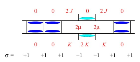
Figure 1: Illustration of the different Ising parameters appearing in the Hamiltonian $\beta H$. Open (closed) base pairs are coded by a spin $\sigma=+1$ ($-1$). The energies indicate the cost of opening base-pairs with respect to the ground state where all $\sigma$ are set to $+1$. The first line shows the cost, $2J$, of a domain wall. The second line indicates the energy, $2\mu$, required to open a base pair. The third line gives the difference in stacking energy between a segment of dsDNA and a denaturated one: dark (light) blue cigars indicate stacked state in dsDNA (in ssDNA) and the absence of dots indicates the destacking of adjacent base pairs, which is already taken into account by the $J$ contribution.

The term in $\tilde{J}$ accounts for the local destacking energy ($2\tilde{J}$) of a domain wall (where $\sigma_{i}$ passes from one value to another). The term in $\tilde{K}$ accounts for the difference in stacking energy between a segment of dsDNA and of a denaturation bubble. The last term gives the energy (2$\tilde{\mu}$) required to create a link in the state $\sigma_{i}=-1$ (a B link or broken bond). We write a dimensionless Hamiltonian $\beta H[\sigma_{i},\Omega_{i}]$, where $\beta=1/(k_{B}T)$, which thus contains the dimensionless parameters $\kappa_{i+1,i}\equiv\beta{\tilde{\kappa}}_{i+1,i}$, $J\equiv\beta\tilde{J}$, $K\equiv\beta\tilde{K}$, and $\mu\equiv\beta\tilde{\mu}$. The local rigidity is

$$\kappa_{i+1,i}=\left\{\begin{array}[]{ll}\kappa_{U}&{\rm for\;U-U\;n.n.}\\ \kappa_{B}&{\rm for\;B-B\;n.n.}\\ \kappa_{UB}&{\rm for\;U-B\;or\;B-U\;n.n.}\\ \end{array}\right.$$ (3)

where “U-U n.n.”, etc. denotes nearest neighbor link types. In terms of the Ising field $\sigma_{i}$

$$\kappa_{i+1,i}=\frac{1}{4}(\kappa_{U}+\kappa_{B}-2\kappa_{UB})\sigma_{i+1}\sigma_{i}+\frac{1}{4}(\kappa_{U}-\kappa_{B})(\sigma_{i+1}+\sigma_{i})+\frac{1}{4}(\kappa_{U}+\kappa_{B}+2\kappa_{UB}).$$ (4)

We identify the B state with two identical non-interacting single DNA strands, ssDNA, each with a local rigidity equal to $\kappa_{B}/2$. From Eqs. (1) and (4), the result of the coupling between Ising and tangent variables can already be predicted: both the destacking and stacking parameters $\tilde{J}$ and $\tilde{K}$ will be modified by the two first terms in Eq. (4) which have exactly the same functional form in $\sigma_{i}$, whereas $\tilde{\mu}$ will remain unchanged. Moreover, when all the bending rigidities are equal, $\kappa_{U}=\kappa_{B}=\kappa_{UB}$, the two first terms in Eq. (4) disappear and the Hamiltonian (1) decouples into a pure Ising Hamiltonian and a pure DWLC one (isomorphic to a 1D classical Heisenberg model for magnetism fisher ): $H[\sigma_{i},{\bf{t}}_{i}]=H_{\rm DWLC}[{\bf t}_{i}]+H_{\rm I}[\sigma_{i}]$. In the language of magnetism the model studied here is a classical coupled Heisenberg-Ising spin chain. Although pure effective Ising models have been used extensively to model helix-coil and denaturation (melting) transitions in macromolecules, it was necessary to introduce phenomenologically an effective temperature-dependent chemical potential to obtain a melting transition. A key feature of the coupled model used here is that a melting transition will emerge naturally in the effective Ising model obtained by integrating out the chain conformational degrees of freedom.

The quantities that we will use to study the behavior of the coupled system are the mean of the internal state variable (“magnetization” in spin language)

$$c\equiv\frac{1}{N}\sum_{i=1}^{N}\,\sigma_{i},$$ (5)

the local state average, $\langle\sigma_{i}\rangle$, correlation functions for the Ising variables, $\langle{\sigma_{i+r}\sigma_{i}}\rangle$, and the chain tangent vectors, $\langle{{\bf{t}}_{i+r}\cdot{\bf{t}}_{i}}\rangle$, and the mean square radius $R\equiv\langle{\bf R}^{2}\rangle^{1/2}$. These correlation functions measure the extent of cooperativity exhibited by the coupled system: e.g., the size of the B (U) domains below (above) the melting temperature, and the length scale on which the chain remains rigid. The concentration of U and B links is given by

$$\varphi_{B}(N,T)=\frac{1-\langle c\rangle(N,T)}{2}=1-\varphi_{U}(N,T).$$ (6)

Once the type of homopolymeric DNA is chosen, the bare Ising parameters and the chain bending rigidities can be considered fixed, and therefore $\langle c\rangle$, $\varphi_{U}$, and $\varphi_{B}$ become functions of the experimental control parameters, namely temperature, $T$, and chain length, $N$. For a pure U chain $\varphi_{U}=1$ and $\varphi_{B}=0$; for a pure B chain $\varphi_{U}=0$ and $\varphi_{B}=1$. A chain with a finite concentration of bubbles (B links) will have $\varphi_{B}>0$ and the melting temperature $T_{m}<\infty$, if it exists, will be defined by $\varphi_{U}(T_{m})=\varphi_{B}(T_{m})=1/2$ . The equilibrium statistical average of a quantity $\mathcal{O}=\mathcal{O}[\sigma_{i},\Omega_{i}]$ that depends on the fluctuating degrees of freedom, $[\sigma_{i},\Omega_{i}]$, is given by

$$\langle\mathcal{O}\rangle\equiv\frac{(4\pi)^{N}}{\mathcal{Z}}\sum_{\{\sigma_{i}=\pm 1\}}\,\prod_{i=1}^{N}\,\int\frac{d\Omega_{i}}{4\pi}\mathcal{O}[\sigma_{i},\Omega_{i}]e^{-\beta H[\sigma_{i},\Omega_{i}]},$$ (7)

where

$$\mathcal{Z}=(4\pi)^{N}\sum_{\{\sigma_{i}\}}\,\prod_{i=1}^{N}\,\int\frac{d\Omega_{i}}{4\pi}e^{-\beta H[\sigma_{i},\Omega_{i}]}$$ (8)

is the partition function. The partition and correlation functions for the coupled system can be calculated using transfer matrix techniques. For example, the partition function can be written as

$$\mathcal{Z}=(4\pi)^{N}\sum_{\{\sigma_{i}\}}\,\prod_{i=1}^{N}\,\int\frac{d\Omega_{i}}{4\pi}\langle{V|\sigma_{1}}\rangle\langle\sigma_{1}|\hat{P}(\Omega_{1},\Omega_{2})|\sigma_{2}\rangle\cdots\langle\sigma_{N-1}|\hat{P}(\Omega_{N-1},\Omega_{N})|\sigma_{N}\rangle\langle{\sigma_{N}|V}\rangle,$$ (9)

where the transfer kernel that appears $N-1$ times in Eq. (9), is given by

$$\hat{P}(\Omega_{i},\Omega_{i+1})=\left(\begin{array}[]{*{20}c}{e^{\kappa_{U}[\cos(\gamma_{i+1,i})-1]+J+K+\mu}}&{e^{\kappa_{UB}[\cos(\gamma_{i+1,i})-1]-J}}\\ {e^{\kappa_{UB}[\cos(\gamma_{i+1,i})-1]-J}}&{e^{\kappa_{B}[\cos(\gamma_{i+1,i})-1]+J-K-\mu}}\\ \end{array}\right).$$ (10)

It is written in the canonical base $|U\rangle=|+1\rangle$ and $|B\rangle=|-1\rangle$ of the U and B states. The end vector

$$|V\rangle=e^{\mu/2}|U\rangle+e^{-\mu/2}|B\rangle$$ (11)

enters in order to take care of the free chain boundary conditions. Different boundary conditions could be easily handled in a similar way, for instance for closed (open) ends, $|V\rangle=|U\rangle$ ($|B\rangle$) and all the following results not explicitly using Eq. (11) remain valid.

Before presenting the full transfer matrix method, we first show that the partition function and averages of any quantities depending only on the Ising variables can be obtained by examining the effective Ising model obtained by integrating over the chain conformational degrees of freedom (the link tangent vectors) in Eq. (9). The problem reduces to that of an effective Ising model with an “effective free energy” $H_{\rm I,eff}^{(0)}$ containing renormalized parameters. This method works because, for the coupled Ising-chain system, the rotational symmetry is not broken (absence of a force term $\propto{\bf t}_{i}\cdot{\bf\hat{z}}$ in the Hamiltonian nelson ; Nelson03 ). Hence the matrix obtained by integrating the kernel $\hat{P}(\Omega_{i},\Omega_{i+1})$ in Eq. (9) is the same for any site $i$. We thus are able to carry out the solid angle integrations in sequential fashion by using the $(i+1)^{\rm th}$ tangent vector as the polar axis for the $i^{\rm th}$ solid angle integration. The solid angle integrated transfer matrix is

$$\hat{P}_{\rm I,eff}^{(0)}=\int\frac{{d\Omega_{i}}}{{4\pi}}\hat{P}(\Omega_{i},\Omega_{i+1})=\left({\begin{array}[]{*{20}c}{e^{-G_{0}(\kappa_{U})+J+K+\mu}}&{e^{-G_{0}(\kappa_{UB})-J}}\\ {e^{-G_{0}(\kappa_{UB})-J}}&{e^{-G_{0}(\kappa_{B})+J-K-\mu}}\\ \end{array}}\right)$$ (12)

where $G_{0}(\kappa)$ is the (dimensionless) Helmholtz free energy of a single joint (two-link) subsystem with rigidity $\kappa$ (either U-U, B-B, U-B or B-U):

$$G_{0}(\kappa)=-\ln\left\{\int\frac{{d\Omega}}{{4\pi}}\exp[\kappa(\cos(\theta)-1)]\right\}=\kappa-\ln\left[\frac{\sinh(\kappa)}{\kappa}\right],$$ (13)

an increasing function of $\kappa$, varying linearly with $\kappa$ for $\kappa\ll 1$ (high $T$) and as $\ln(2\kappa)$ for $\kappa\gg 1$ (low $T$ entropy dominated regime where the spin wave approximation for the chain degrees of freedom is valid). The effective transfer matrix $\hat{P}_{\rm I,eff}^{(0)}$ can be written in Ising form using the renormalized Ising parameters, $J_{0}$, $K_{0}$ and the prefactor $\exp(-\Gamma_{0})$, all depending on chain rigidities:

$$\hat{P}_{\rm I,eff}^{(0)} = e^{-\Gamma_{0}}\left({\begin{array}[]{*{20}c}{e^{\mu+K_{0}+J_{0}}}&{e^{-J_{0}}}\\ {e^{-J_{0}}}&{e^{-\mu-K_{0}+J_{0}}}\\ \end{array}}\right)$$ (16)

$$J_{0} \equiv J-\frac{1}{4}\left[G_{0}(\kappa_{U})+G_{0}(\kappa_{B})-2G_{0}(\kappa_{UB})\right]$$ (17)

$$K_{0} \equiv K-\frac{1}{2}\left[G_{0}(\kappa_{U})-G_{0}(\kappa_{B})\right]$$ (18)

$$\Gamma_{0} \equiv \frac{1}{4}\left[{G_{0}(\kappa_{U})+G_{0}(\kappa_{B})+2G_{0}(\kappa_{UB})}\right].$$ (19)

In the limit of high temperature, the chain tangents will be completely decorrelated and the uninteresting renormalizations of $J$ and $K$ arise solely from $\kappa_{i+1,i}$ (Eq. 4), in agreement with Eqs. (17) and (18), as revealed by the linear dependence of $G_{0}(\kappa)$ on $\kappa$ in this limit. It is rather in the opposite limit of low temperatures and therefore strongly correlated chain tangents that the bending entropy driven denaturation transition arises.

The full partition function, $\mathcal{Z}=\mathcal{Z}_{\rm I,eff}^{(0)}$, in Ising transfer matrix notation,

$$\mathcal{Z}_{\rm I,eff}^{(0)}=(4\pi)^{N}\sum_{\{\sigma_{i}\}}\,\langle{V|\sigma_{1}}\rangle\langle\sigma_{1}|\hat{P}_{\rm I,eff}^{(0)}|\sigma_{2}\rangle\cdots\langle\sigma_{N-1}|\hat{P}_{\rm I,eff}^{(0)}|\sigma_{N}\rangle\langle{\sigma_{N}|V}\rangle,$$ (20)

can be rewritten explicitly in terms of an effective Ising free energy, $H_{\rm I,eff}^{(0)}$:

$$\mathcal{Z}_{\rm I,eff}^{(0)}=(4\pi)^{N}e^{-(N-1)\Gamma_{0}}\sum_{\{\sigma_{i}\}}\,e^{-\beta H_{\rm I,eff}^{(0)}[\sigma_{i}]}$$ (21)

where $H_{\rm I,eff}^{(0)}=H_{\rm I}(\tilde{J}_{0},\tilde{K}_{0},\tilde{\mu})$:

$$\beta H_{\rm I,eff}^{(0)} = -J_{0}\sum_{i=1}^{N-1}\,\sigma_{i+1}\sigma_{i}-\frac{K_{0}}{2}\sum_{i=1}^{N-1}\,(\sigma_{i+1}+\sigma_{i})-\mu\sum_{i=1}^{N}\,\sigma_{i}$$ (22)

$$= -J_{0}\sum_{i=1}^{N-1}\,\sigma_{i+1}\sigma_{i}-\frac{L_{0}}{2}\sum_{i=1}^{N-1}\,(\sigma_{i+1}+\sigma_{i})-\frac{\mu}{2}(\sigma_{1}+\sigma_{N})$$

with

$$L_{0}\equiv\mu+K_{0}=\mu+K-\Delta G_{0}^{UB}/2,$$ (23)

and $\Delta G_{0}^{UB}\equiv G_{0}(\kappa_{U})-G_{0}(\kappa_{B})$. Because $H_{\rm I,eff}^{(0)}$ depends on the temperature, it cannot be considered as an Ising state energy, but rather as an effective free energy obtained by integrating out the chain subsystem (cf. discussion concerning levels of theoretical study in the Introduction).

When two links open the renormalized stacking energy of the links is $K_{0}$, which is smaller than $K$ by the difference in bending free energy between U-B and B-B joints. The second form of $\beta H_{\rm I,eff}^{(0)}$ in Eq. (22) shows that the effective chemical potential of one interior base pair is renormalized to $L_{0}$. If the gain in the one link bending free energy in going from U to B, $\Delta G_{0}^{UB}$, is greater than the intrinsic energy, $2(\tilde{\mu}+\tilde{K})$, needed to break a closed interior bond, then the effective interior joint chemical potential $L_{0}$ can become negative, signaling a change in stability of U and B states. The end links $(i=1,N)$, however, feel a different chemical potential, $\mu+K_{0}/2$, which is larger than $L_{0}$ in the case of interest ($\kappa_{U}>\kappa_{B}$). This end-interior asymmetry, along with the extra bubble initiation energy due to the second domain wall, are reflected in the difference between the “effective free energy” needed to create an $n$-bubble at a chain end,

$$\beta\Delta G_{{\rm{end}}}^{(n)}=2J_{0}-K_{0}+2nL_{0}$$ (24)

and in the chain interior

$$\beta\Delta G_{{\rm{int}}}^{(n)}=4J_{0}+2nL_{0},$$ (25)

which is higher than for an end link by $2J_{0}+K_{0}$. As will be confirmed in section VIII, this difference in effective free energy suggests that at sufficiently low $T$ bond melting will begin at the chain ends. Written out in greater detail, Eq. (25) leads to

$$\Delta G_{{\rm{int}}}^{(n)}=4\tilde{J}_{0}+2nk_{B}TL_{0}=4\tilde{J}+2n(\tilde{\mu}+\tilde{K})-k_{B}T[G_{0}(\kappa_{U})+G_{0}(\kappa_{B})-2G_{0}(\kappa_{UB})]-nk_{B}T\Delta G_{0}^{UB}.$$ (26)

In the uncoupled limit ($\kappa_{U}=\kappa_{B}=\kappa_{UB}$) only the first two (temperature independent) terms survive. Although this end-interior asymmetry plays no role in the limit of an infinite chain $(N\to\infty)$, it will play an essential role in determining how bond melting varies with temperature and bond location (melting maps) and how the melting temperature varies with chain size. These finite size effects are discussed in detail in section VIII.

Because the renormalized Ising parameters depend on the chain parameters, the coupled model does not in general have the same behavior as the uncoupled one. Indeed, since $G_{0}(\kappa)$ is an increasing function of $\kappa$ and $\kappa_{U}\gg\kappa_{B}$ for dsDNA, if the difference between $\kappa_{U}$ and $\kappa_{B}$ is sufficiently large, then at a certain temperature, $T_{m}^{\infty}$, the effective interior bubble chemical potential, $L_{0}$, can vanish. Provided that this temperature be sufficiently low for thermal disorder to be weak and end effects due to the finite size of the chain to be unimportant, the state of the system will flip from nearly pure U for $T<T_{m}^{\infty}$, where $L_{0}>0$, to nearly pure B for $T>T_{m}^{\infty}$, where $L_{0}<0$ . Precisely at $T=T_{m}^{\infty}$, there will be, on average, as many closed as open bonds and $\varphi_{B,\infty}=\varphi_{U,\infty}=1/2$, where $\varphi_{B,\infty}(T)\equiv\lim_{N\to\infty}\varphi_{B}(N,T)$, etc. This transition (strictly speaking a crossover), which can be extremely sharp under some circumstances (see below), can be interpreted as a melting or denaturation transition. From the above analysis, we see clearly that it is the difference in free energy between U-U and B-B joints, $\Delta G_{0}^{UB}$, that drives the melting transition. We will see below, moreover, that if $\kappa_{U}$ and $\kappa_{B}$ are much greater than one, then the spin wave approximation is valid, and the entropy term in $\Delta G_{0}^{UB}$ dominates. We will see in section VII that this is actually the case for real DNA.

By calculating the average of the product of the cosines of the $N-1$ angles, $\prod_{i}\cos(\gamma_{i+1,i})$ and using the same technique used above for $\mathcal{Z}_{\rm I,eff}^{(0)}$, we can define another effective model, but now with partition function

$$\mathcal{Z}_{\rm I,eff}^{(1)}=\mathcal{Z}\left\langle\prod_{i=1}^{N-1}\,{\bf t}_{i+1}\cdot{\bf t}_{i}\right\rangle.$$ (27)

This expression can be written in Ising transfer matrix form as

$$\mathcal{Z}_{\rm I,eff}^{(1)}=(4\pi)^{N}\sum_{\{\sigma_{i}\}}\,\langle{V|\sigma_{1}}\rangle\langle\sigma_{1}|\hat{P}_{\rm I,eff}^{(1)}|\sigma_{2}\rangle\cdots\langle{\sigma_{N-1}|\hat{P}_{\rm I,eff}^{(1)}|\sigma_{N}}\rangle\langle{\sigma_{N}|V}\rangle,$$ (28)

where

$$\hat{P}_{\rm I,eff}^{(1)} = \int\frac{d\Omega_{i}}{4\pi}\cos(\gamma_{i+1,i})\hat{P}(\Omega_{i},\Omega_{i+1})=e^{-\Gamma_{1}}\left({\begin{array}[]{*{20}c}{e^{\mu+K_{1}+J_{1}}}&{e^{-J_{1}}}\\ {e^{-J_{1}}}&{e^{-\mu-K_{1}+J_{1}}}\\ \end{array}}\right)$$ (31)

$$J_{1} \equiv J-\frac{1}{4}[G_{1}(\kappa_{U})+G_{1}(\kappa_{B})-2G_{1}(\kappa_{UB})]$$ (32)

$$K_{1} \equiv \mu-\frac{1}{2}[G_{1}(\kappa_{U})-G_{1}(\kappa_{B})]$$ (33)

$$\Gamma_{1} \equiv \frac{1}{4}.$$ (34)

The function $G_{1}(\kappa)=-\ln\{\int\frac{d\Omega}{4\pi}\cos(\theta)\exp[\kappa(\cos(\theta)-1)]\}$ is related to the tangent-tangent correlation function between two adjacent monomers (isolated 2-link sub-system) with rigidity $\kappa$:

$$\left\langle{{\bf{t}}_{1}\cdot{\bf{t}}_{2}}\right\rangle_{{\rm{2-link}}}=\left\langle{\cos(\theta)}\right\rangle_{{\rm{2-link}}}=\exp\left[-G_{1}(\kappa)+G_{0}(\kappa)\right]=u(\kappa)=\coth(\kappa)-1/\kappa,$$ (35)

which is the Langevin function joyce . It increases with $\kappa$, varying as $\kappa/3$ for $\kappa\ll 1$ and as $1-1/\kappa$ for $\kappa\gg 1$. This asymptotic behavior corresponds to $G_{1}(\kappa)-G_{0}(\kappa)$ varying as $\ln(3/\kappa)$ for $\kappa\ll 1$ and as 1/$\kappa$ for large $\kappa$. For a pure chain (U or B) $\langle\cos(\theta)\rangle_{2-{\rm link}}$ is equal to the nearest-neighbor tangent correlation function $\langle{\bf t}_{i+1}\cdot{\bf t}_{i}\rangle=\exp(-1/\xi_{p})$ with persistence length

$$\xi_{p}(\kappa)=-1/\ln[u(k)]=[G_{1}(\kappa)-G_{0}(\kappa)]^{-1}.$$ (36)

In the high $\kappa$ (spin wave) approximation, we obtain $\xi_{p}\simeq\kappa$, as expected.

The partition function can be rewritten explicitly in terms of an effective Ising free energy, $H_{\rm I,eff}^{(1)}$:

$$\mathcal{Z}_{\rm I,eff}^{(1)}=(4\pi)^{N}e^{-(N-1)\Gamma_{1}}\;\sum_{\{\sigma_{i}\}}\,e^{-\beta H_{\rm I,eff}^{(1)}[\sigma_{i}]},$$ (37)

where

$$\beta H_{\rm I,eff}^{(1)}=-\sum_{i=1}^{N-1}\,\left[J_{1}\sigma_{i+1}\sigma_{i}+\frac{L_{1}}{2}(\sigma_{i+1}+\sigma_{i})\right]-\frac{\mu}{2}(\sigma_{1}+\sigma_{N}).$$ (38)

By repeatedly using the vector identity $({\bf a}\cdot{\bf c})({\bf b}\cdot{\bf d})=({\bf a}\cdot{\bf d})({\bf b}\cdot{\bf c})-({\bf a}\times{\bf b})\cdot({\bf c}\times{\bf d})$ for ${\bf{a}}\cdot{\bf{b}}={\bf{t}}_{i+1}\cdot{\bf{t}}_{i}$, etc., along with the property that averages of cross products, $\langle{\bf{t}}_{i+1}\times{\bf{t}}_{i}\rangle$, are zero (and that $\left|{{\bf{t}}_{i}}\right|^{2}=1$), the partition function $\mathcal{Z}_{\rm I,eff}^{(1)}$ can be written as the product of the end-end tangent-tangent correlation function, $\langle{\bf{t}}_{1}\cdot{\bf{t}}_{N}\rangle$, and the effective Ising partition function, $\mathcal{Z}_{\rm I,eff}^{(0)}$:

$$\mathcal{Z}_{\rm I,eff}^{(1)}=\left\langle{\bf{t}}_{1}\cdot{\bf{t}}_{N}\right\rangle\mathcal{Z}_{\rm I,eff}^{(0)}.$$ (39)

When $\kappa_{U}=\kappa_{B}=\kappa_{UB}=\kappa$, we recover the pure chain tangent-tangent correlation function:

$$\langle{\bf{t}}_{1}\cdot{\bf{t}}_{N}\rangle=\frac{\mathcal{Z}_{\rm I,eff}^{(1)}}{\mathcal{Z}_{\rm I,eff}^{(0)}}\to\left\{\frac{\exp[-G_{1}(\kappa)]}{\exp[-G_{0}(\kappa)]}\right\}^{N-1}=\exp\left[-(N-1)/\xi_{p}(\kappa)\right].$$ (40)

Coming back to the difference in (dimensionless) free energy $\Delta G_{0}^{UB}$, we can show that at room temperature it is dominated by its entropic part. Indeed, $G_{0}(\kappa)$ can be split into an average (dimensionless) energy and average entropy contribution, $G_{0}(\kappa)=E_{0}(\kappa)-S_{0}(\kappa)/k_{B}$, where $E_{0}(\kappa)=\beta\,\partial G_{0}/\partial\beta=\kappa\,\partial G_{0}(\kappa)/\partial\kappa$. Hence, the average energy of a two-link system can be written in terms of $G_{0}$ and $G_{1}$:

$$E_{0}(\kappa)=\kappa\left[1-\exp\left(-G_{1}(\kappa)+G_{0}(\kappa)\right)\right]=\kappa\left[1-\exp\left(-1/\xi_{p}(\kappa)\right)\right]=\kappa\left[1-u(\kappa)\right],$$ (41)

and therefore $\Delta E_{0}^{UB}\equiv E_{0}(\kappa_{U})-E_{0}(\kappa_{B})=(\kappa_{U}-\kappa_{B})-[\kappa_{U}u(\kappa_{U})-\kappa_{B}u(\kappa_{B})]$. Because the function $u(\kappa)$ tends to 1, $\Delta E_{0}^{UB}\to 0$, and therefore for temperatures low enough for the spin wave approximation to be valid for both U-U and B-B links, we see that $\Delta G_{0}^{UB}\simeq-\Delta S_{0}^{UB}/k_{B}$. Indeed in this approximation, the Hamiltonian is Gaussian and equipartition of energy occurs: $\langle\tilde{E}\rangle\sim\beta^{-1}\Rightarrow\langle E\rangle=\beta\langle\tilde{E}\rangle\sim 1$. In this case the melting transition, if it exists, will be driven overwhelmingly by the difference in entropy between U-U and B-B joints. As done for $\Delta G_{0}^{UB}$, the difference in (dimensionless) free energy $\Delta G_{1}^{UB}$ can be split into an average (dimensionless) energy and average entropy contribution using the same formulæ as above. If $L_{1}=0$ at a certain temperature, $T_{1}^{\infty}$, then we can expect another type of “melting” transition, now driven by the free energy difference $\Delta G_{1}^{UB}\equiv G_{1}(\kappa_{U})-G_{1}(\kappa_{B})$. We return to this point below.

It should be noticed that the above processus could in principle be carried on (with increasing difficulty) to calculate higher order correlation functions quantities. Hence these effective Ising models give information on multi-point tangent-tangent correlation functions. In the next section we obtain the solutions to the two effective Ising models.

III Solution of the two Ising models

The effective Ising partition and correlation functions can be obtained using well-known Ising transfer matrix techniques nelson . In order to treat in parallel $\mathcal{Z}_{\rm I,eff}^{(0)}$ and $\mathcal{Z}_{\rm I,eff}^{(1)}$, we introduce the index $l=0,1$ and compute the associated partition function $\mathcal{Z}_{\rm I,eff}^{(l)}$. This index will be useful in Section V where we introduce the transfer matrix approach. We need the eigenvectors and eigenvalues of the transfer matrices: $\hat{P}_{\rm I,eff}^{(l)}|{\psi^{(l)}}\rangle=\lambda_{l}|\psi^{(l)}\rangle$, where the expressions for $\hat{P}_{\rm I,eff}^{(l)}$ are given in Eqs. (12,31). The eigenvalues are

$$\lambda_{l,\pm}=e^{J_{l}-\Gamma_{l}}\left\{{\cosh(L_{l})\pm\left[\sinh^{2}(L_{l})+e^{-4J_{l}}\right]^{1/2}}\right\}$$ (42)

and they obey the inequality $\lambda_{l,+}>\lambda_{l,-}$. The two orthonormal eigenvectors, $|\psi^{(l)}\rangle$, are

$$|l,+\rangle=\frac{1}{\sqrt{2\gamma_{l}}e^{J_{l}}}\left(a_{l}|U\rangle+a_{l}^{-1}|B\rangle\right)\quad\mathrm{and}\quad|l,-\rangle=\frac{1}{\sqrt{2\gamma_{l}}e^{J_{l}}}\left(a_{l}^{-1}|U\rangle-a_{l}|B\rangle\right),$$ (43)

where

$$\gamma_{l}=\left[\sinh^{2}(L_{l})+e^{-4J_{l}}\right]^{1/2}\quad\mathrm{and}\quad a_{l}=e^{J_{l}}\left[\sinh(L_{l})+\gamma_{l}\right]^{1/2}.$$ (44)

The transfer matrices can be expanded in terms of the eigenvectors

$$\hat{P}_{\rm I,eff}^{(l)}=\sum_{\tau=\pm}{\lambda_{l,\tau}\left|{l,\tau}\right\rangle}\left\langle{l,\tau}\right|.$$ (45)

Using the decomposition of the Ising $(2\times 2)$ identity matrix, $\hat{I}_{I}=\sum_{\tau}|l,\tau\rangle\langle l,\tau|$ the orthonormality of the eigenvectors $|l,\tau\rangle$ for each value of $l$ [i.e., $\langle l,\tau|l,\tau^{\prime}\rangle=\delta_{\tau,\tau^{\prime}}$], and the forms Eqs. (20,28) for the effective Ising partition functions, we then find

$$\mathcal{Z}_{\rm I,eff}^{(l)}=(4\pi)^{N}\left\langle V\right|\left[\hat{P}_{\rm I,eff}^{(l)}\right]^{N-1}\left|V\right\rangle=(4\pi)^{N}\sum_{\tau=\pm}\lambda_{l,\tau}^{N-1}\langle V|{l,\tau}\rangle^{2}.$$ (46)

The full partition is given by $\mathcal{Z}=\mathcal{Z}_{\rm I,eff}^{(0)}$. The matrix elements, $\langle V|{l,\tau}\rangle$, entering Eq. (46) can be obtained explicitly from Eqs. (11), (43), and (44).

When $\kappa_{U}=\kappa_{B}=\kappa_{UB}$, the system decouples, but the pure Ising model with temperature-independent parameters, $\tilde{J}$, $\tilde{K}$ and $\tilde{\mu}$, exhibits neither a second order phase transition at a finite temperature in zero “field” ($\tilde{\mu}+\tilde{K}=0$), nor a melting transition at a finite temperature for $\tilde{\mu}+\tilde{K}>0$. Indeed, there can be no melting transition because the inequality $\varphi_{B}<1/2$ holds over the whole temperature range. At low temperatures, ${\sinh(\mu+K)\gg e^{-2J}}$, and the system is ordered with $\varphi_{U}\simeq 1$ and $\varphi_{B}\simeq 0$. As the temperature is raised, denaturation bubbles are thermally excited, with a cross-over when $\sinh(\mu+K)\simeq e^{-2J}$, or roughly $\beta^{\prime}=(k_{B}T^{\prime})^{-1}\simeq({\tilde{\mu}+\tilde{K}+2\tilde{J}})^{-1}$. At higher temperatures ($\sinh(\mu+K)\ll e^{-2J}$), the average “magnetization” monotonously approaches a completely thermally disordered state with $\langle c\rangle=0$ and $\varphi_{U}=\varphi_{B}=1/2$. Note that this regime is not reached for DNA since as we will see below, $T^{\prime}\simeq 8\,T_{m}$ and the model is certainly no longer valid for such high temperatures. By contrast, the coupled Ising-chain model will exhibit a very different behavior, with a finite temperature melting transition. In the following we implicitly assume that all temperatures of interest obey $T\ll T^{\prime}$.

Although the eigenvectors $|l,\tau\rangle$ are orthogonal in $\tau$ for the same value of $l$, this is not necessarily the case for different values of $l$ (as we will see below, this is a consequence of the difference in rotational symmetry). In general, depending on the values of the temperature-dependent effective Ising parameters, $L_{l}$ and $J_{l}$, the eigenvectors are complicated mixtures of the canonical basis states, $|U\rangle$ and $|B\rangle$. These eigenvectors and their corresponding eigenvalues can, however, be simplified in two important limits:

• For sufficiently low or high temperatures, below or above the transition temperature, $T_{l}^{\infty}$ (at which $L_{l}$ vanishes), the inequality $\sinh^{2}(L_{l})\gg e^{-4J_{l}}$ is obeyed (the experimental melting temperature for infinite chains is thus $T_{m}^{\infty}\equiv T_{0}^{\infty}$). As a consequence, the off-diagonal (domain-wall or “tunneling”) terms in $\hat{P}_{\rm I,eff}^{(l)}$ can be neglected and the eigenvectors reduce asymptotically to the canonical ones, with the mapping depending on the sign of $L_{l}$: $|l,+\rangle\simeq|U\rangle$ and $|{l,-}\rangle\simeq-|B\rangle$ for $L_{l}>0$ and $|{l,-}\rangle\simeq|U\rangle$ and $|{l,+}\rangle\simeq|B\rangle$ for $L_{l}<0$. In this limit of strong cooperativity, the eigenvalues reduce to

  $$\lambda_{l,\pm}\simeq\exp\left({J_{l}\pm\left|{L_{l}}\right|-\Gamma_{l}}\right)\quad\mathrm{for}\quad\sinh^{2}(L_{l})\gg e^{-4J_{l}}$$ (47)

  and therefore the pure U state is strongly favored if $L_{l}>0$ and the B state if $L_{l}<0$, because

  $$\frac{{\lambda_{l,+}}}{{\lambda_{l,-}}}\simeq\exp\left({2\left|{L_{l}}\right|}\right)\quad\mathrm{for}\quad\sinh^{2}(L_{l})\gg e^{-4J_{l}}.$$ (48)

  By introducing the following eigenvalues for pure $U$ and pure $B$

  $$\lambda_{l,U} \equiv \exp[J+\mu-G_{l}(\kappa_{U})]$$ (49)

  $$\lambda_{l,B} \equiv \exp[J-\mu-G_{l}(\kappa_{B})]$$ (50)

  and using the definitions of $J_{l},L_{l}$, and $\Gamma_{l}$, these limiting forms for the eigenvalues can be further simplified ($\sinh^{2}(L_{l})\gg e^{-4J_{l}}$):

  $$\begin{array}[]{l}\lambda_{l,+}\simeq\lambda_{l,U}\\ \lambda_{l,-}\simeq\lambda_{l,B}\\ \end{array}\quad\mathrm{for}\quad L_{l}>0\quad\mathrm{and}\quad\begin{array}[]{l}\lambda_{l,+}\simeq\lambda_{l,B}\\ \lambda_{l,-}\simeq\lambda_{l,U}\\ \end{array}\quad\mathrm{for}\quad L_{l}>0.$$ (51)

• For temperatures at or very near the transition temperature, however, the opposite inequality $\sinh^{2}(L_{l})\ll e^{-4J_{l}}$ holds and $L_{l}$ can be set to zero in Eqs. (42)–(44): the eigenvectors then reduce to symmetric and anti-symmetric, superpositions of the canonical basis vectors, $|U\rangle$ and $|B\rangle$:

  $$\left|{l,\pm}\right\rangle\simeq\frac{1}{\sqrt{2}}\left({\left|U\right\rangle\pm\left|B\right\rangle}\right)\quad\mathrm{for}\quad\sinh^{2}(L_{l})\ll e^{-4J_{l}}$$ (52)

  with eigenvalues

  $$\lambda_{l,\pm}\simeq e^{-\Gamma_{l}}(e^{J_{l}}\pm e^{-J_{l}})\quad\mathrm{for}\quad\sinh^{2}(L_{l})\ll e^{-4J_{l}}.$$ (53)

  In this limit of weak cooperativity the eigenvalue ratio is approximately $\lambda_{l,+}/\lambda_{l,-}\simeq\coth(J_{l})$ and the behavior of the system is dominated by the domain walls. The average behavior for large $N$, which is governed by the ground symmetrical state, shows vanishing average for the mean of the Ising state variable (or magnetization in spin language) (for $l=0$ and $N\to\infty$, $\varphi_{U}\simeq\varphi_{B}\simeq 1/2$, since there is no spontaneous second order phase transition for the 1D zero field Ising model).

The exact results for the eigenvalues and eigenvectors interpolate smoothly between the above simplified results obtained far from and close to $T_{l}^{\infty}$ (Fig. 2).

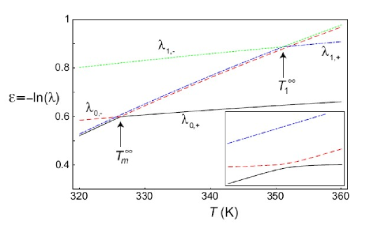
Figure 2: “Energies” $\varepsilon_{l,\pm}=-\ln(\lambda_{l,\pm})$ for $l=0,1$ in the quantum formalism (related to the Landau-Zener problem) vs. temperature (for parameter values used in section VII to fit experimental melting data: $\tilde{\mu}=4.46$ kJ/mol, $\tilde{J}=9.13$ kJ/mol and $\tilde{K}=0$). We observe that far from the two transition temperatures, the eigenvalues reduce to the limiting forms Eq. (51). The inset is a zoom close to $T_{m}^{\infty}$ showing the level repulsion between the branches ($0,\pm$). A similar level repulsion occurs near $T_{1}^{\infty}$ between the branches ($1,\pm$).

Using Eq. (11), these limiting forms can be used to obtain simple approximations for the following important matrix elements :

$$\langle V|0,+\rangle=\left\{\begin{array}[]{ll}e^{\mu/2},&T<T_{m}^{\infty}\\ \sqrt{2}\cosh(\mu/2),&T=T_{m}^{\infty}\\ e^{-\mu/2},&T>T_{m}^{\infty}\\ \end{array}\right.,$$ (54)

$$\langle V|0,-\rangle=\left\{\begin{array}[]{ll}-e^{-\mu/2},&T<T_{m}^{\infty}\\ \sqrt{2}\sinh(\mu/2),&T=T_{m}^{\infty}\\ e^{\mu/2},&T>T_{m}^{\infty}.\\ \end{array}\right.$$ (55)

The limiting forms for $\langle V|0,-\rangle$ reveal that this matrix element is negative for low temperature and positive at $T_{m}^{\infty}$ and therefore must pass through zero at a temperature $T^{*}$ lower than $T_{m}^{\infty}$. This special temperature will be studied in detail in the section concerning finite size effects (Section VIII).

If a melting transition exists at a finite temperature, $T_{m}^{\infty}$, then $L_{0}$ will go from a positive value below $T_{m}^{\infty}$, through zero at the transition, then to a negative value above $T_{m}^{\infty}$. This temperature dependence for $L_{0}$ is similar to the time dependence of the uncoupled energy levels in the Landau-Zener problem, a quantum 2-state dipole system in an electrical field varying linearly with time landauzener . It is not surprising, therefore, that the 2 branches for the “adiabatic” states of the Landau-Zener problem are equivalent, as the time $t$ varies from $-\infty$ to $+\infty$, to the “eigenenergies”, $\varepsilon_{l,\pm}\equiv-\ln(\lambda_{l,\pm})$, of the states $|{l,\pm}\rangle$ presented above, as the temperature varies from below the transition to above (with the same type of limiting behavior near and far from the transition temperature, $T=T_{l}^{\infty}$, equivalent to $t=0$ in the quantum Landau-Zener problem, see Fig. 2). As in the quantum mechanics of diatomic molecules, eigenenergies possessing the same rotational symmetry (same $l$) cannot cross (level repulsion), although they do reach a point of closest approach at $T_{m}^{\infty}$. As an illustration we show in Fig. 2 the Landau-Zener diagrams, $\varepsilon_{l,\pm}(T)$ for $l=0,1$ and observe level repulsion near $T=T_{m}^{\infty}$ and $T=T_{1}^{\infty}$ for states with same $l$ and the possibility of level crossing for states with different values of $l$.

From the full partition function, we define the (dimensionless) Helmholtz free energy per Ising variable of the coupled system, $F=-N^{-1}\ln\mathcal{Z}$. The average value of the Ising state variable (or “magnetization”) can then be obtained for finite chains using $\langle c\rangle=-\partial F/\partial\mu$, from which $\varphi_{U}$ and $\varphi_{B}$ can be deduced. The expression for $\langle c\rangle$ simplifies in the limit $N\to\infty$, because only the largest of the eigenvalues, $\lambda_{0,+}$, entering in the $l=0$ effective Ising partition function survives:

$$\langle c\rangle\underset{N\to\infty}{\to}\left\langle c\right\rangle_{\infty}\equiv-\frac{\partial f}{\partial\mu}=\frac{\sinh(L_{0})}{[\sinh^{2}(L_{0})+e^{-4J_{0}}]^{1/2}}$$ (56)

where $f={\lim}_{N\to\infty}F=-\ln\lambda_{0,+}$. Equation (56) can then be used to find $\varphi_{U,\infty}$ and $\varphi_{B,\infty}$.

If $L_{0}$ vanishes at a temperature, $T_{m}^{\infty}$, low enough for the $e^{-4J_{0}}$ term in the denominator to be sufficiently small, then the system will undergo a sharp melting transition: $\langle c\rangle_{\infty}$ will jump sharply from $+1$ for $T<T_{m}^{\infty}$ (pure U state) to $-1$ for $T>T_{m}^{\infty}$ (pure B state). The size of $e^{-4J_{0}}$ term in Eq.(56) will determine the width of the transition region,

$$\Delta T_{m}^{\infty}\equiv 2\left|\frac{\partial\left\langle c\right\rangle_{\infty}}{\partial T}\right|_{T_{m}^{\infty}}^{-1}\simeq\frac{2\,k_{B}[T_{m}^{\infty}]^{2}}{\tilde{\mu}}\exp[-2\,J_{0}(T_{m}^{\infty})]$$ (57)

which is exponentially small in $J_{0}(T_{m}^{\infty})$ when $J_{0}(T_{m}^{\infty})\gg 1$.

In a similar manner, from the effective partition function, $\mathcal{Z}_{\rm I,eff}^{(1)}$, we can define the free energy per Ising spin, $F^{(1)}=-N^{-1}\ln\mathcal{Z}_{\rm I,eff}^{(1)}$. A quantity analogous to the average Ising “magnetization”, $\langle c\rangle$, for this partition function can then be obtained for finite chains using

$$\langle c^{(1)}\rangle=-\frac{\partial F^{(1)}}{\partial\mu}=\frac{{\left\langle{c\,({\bf{t}}_{1}\cdot{\bf{t}}_{N})}\right\rangle}}{{\left\langle{\bf{t}}_{1}\cdot{\bf{t}}_{N}\right\rangle}},$$ (58)

from which $\varphi_{U}^{(1)}=(1+\langle c^{(1)}\rangle)/2$ and $\varphi_{B}^{(1)}$ can be obtained. From the definition of $\langle c^{(1)}\rangle$, we see that it is a mixed correlation function that describes how the average system internal state, $c$, is correlated with its external state (chain configuration) via the end-end tangent-tangent correlation function. In the limit of an infinite chain $\langle c^{(1)}\rangle$ reduces to an expression analogous to Eq. (56):

$$\langle c^{(1)}\rangle\underset{N\to\infty}{\to}\langle c^{(1)}\rangle_{\infty}=-\frac{{\partial f^{(1)}}}{{\partial\mu}}=\frac{{\sinh(L_{1})}}{{{\left[{\sinh^{2}(L_{1})+e^{-4J_{1}}}\right]}^{1/2}}},$$ (59)

where $f^{(1)}={\lim}_{N\to\infty}F^{(1)}$. This limiting formula is similar to the one obtained for $\langle c\rangle$ in Eq. (56), which implies that if $L_{1}$ vanishes at a temperature, $T_{1}^{\infty}$, low enough for the $e^{-4J_{1}}$ term in the denominator to be sufficiently small, then the system can undergo a second type of “melting” transition: $\langle c^{(1)}\rangle$ will jump sharply from $+1$ for $T<T_{1}^{\infty}$ (pure $c^{(1)}$ “U” state) to $-1$ for $T>T_{1}^{\infty}$ (pure $c^{(1)}$ “B” state). For $T_{m}^{\infty}<T<T_{1}^{\infty}$, $\langle c^{(1)}\rangle\simeq+1$ while $\langle c\rangle\simeq-1$. This implies that in this temperature range $\langle c\,({\bf t}_{1}\cdot{\bf t}_{N})\rangle\simeq-\langle c\rangle\langle{\bf t}_{1}\cdot{\bf t}_{N}\rangle$. This counter-intuitive result is another manifestation of the non-trivial coupling between internal and external degrees of freedom. The value of the $e^{-4J_{1}}$ term determines again the width of the transition region:

$$\Delta T_{1}^{\infty}\equiv 2\left|\frac{\partial\langle c^{(1)}\rangle_{\infty}}{\partial T}\right|_{T_{1}^{\infty}}^{-1}\simeq\frac{2\,k_{B}[T_{1}^{\infty}]^{2}}{\tilde{\mu}}\exp[-2\,J_{1}(T_{1}^{\infty})].$$ (60)

IV Ising state variable–Ising and chain correlation functions

The average value of the local Ising variable $\left\langle{\sigma_{i}}\right\rangle$ and the 2-point $\left\langle{\sigma_{i+r}\sigma_{i}}\right\rangle$ correlation function can be calculated by starting from the expression Eq. (9) for the partition function and using the property that an insertion of a term $\sigma_{j}$ in the sum of products is equivalent to the insertion of the Pauli matrix in the canonical basis,

$$\hat{\sigma}_{z}=\left(\begin{array}[]{*{20}c}1&0\\ 0&{-1}\\ \end{array}\right)$$ (61)

at the $j^{\rm th}$ position in the product of transfer matrices defining the partition function, Eq. (46). This comes from $\langle\sigma|\hat{\sigma}_{z}|\sigma^{\prime}\rangle=\sigma\delta_{\sigma,\sigma^{\prime}}$ and the equality

$$\sigma_{j}\langle\sigma_{j}|\hat{P}_{\rm I,eff}^{(0)}|\sigma_{j+1}\rangle=\sum_{\sigma=\pm 1}\,\langle\sigma_{j}|\hat{\sigma}_{z}|\sigma\rangle\langle\sigma|\hat{P}_{\rm I,eff}^{(0)}|\sigma_{j+1}\rangle=\langle\sigma_{j}|\hat{\sigma}_{z}\cdot\hat{P}_{\rm I,eff}^{(0)}|\sigma_{j+1}\rangle.$$ (62)

We then find

$$\langle{\sigma_{i}}\rangle = \frac{(4\pi)^{N}}{\mathcal{Z}}\left\langle V\right|\left[{\hat{P}_{\rm I,eff}^{(0)}}\right]^{i-1}\hat{\sigma}_{z}\left[{\hat{P}_{\rm I,eff}^{(0)}}\right]^{N-i}\left|V\right\rangle$$ (63)

$$\langle{\sigma_{i+r}\sigma_{i}}\rangle = \frac{(4\pi)^{N}}{\mathcal{Z}}\left\langle V\right|\left[{\hat{P}_{\rm I,eff}^{(0)}}\right]^{i-1}\hat{\sigma}_{z}\left[{\hat{P}_{\rm I,eff}^{(0)}}\right]^{r}\hat{\sigma}_{z}\left[{\hat{P}_{\rm I,eff}^{(0)}}\right]^{N-r-i}\left|V\right\rangle.$$ (64)

By the same method used for reducing the partition function, we finally obtain

$$\left\langle{\sigma_{i}}\right\rangle = \frac{(4\pi)^{N}}{\mathcal{Z}}\sum_{\tau_{1},\tau_{2}}\langle V|0,\tau_{2}\rangle\lambda_{0,\tau_{2}}^{i-1}\langle 0,\tau_{2}|\hat{\sigma}_{z}|0,\tau_{1}\rangle\lambda_{0,\tau_{1}}^{N-i}\langle{0,\tau_{1}}|V\rangle$$ (65)

$$\left\langle{\sigma_{i+r}\sigma_{i}}\right\rangle = \frac{(4\pi)^{N}}{\mathcal{Z}}\sum_{\tau_{1},\tau_{2},\tau_{3}}\langle V|0,\tau_{3}\rangle\lambda_{0,\tau_{3}}^{i-1}\langle 0,\tau_{3}|\hat{\sigma}_{z}|0,\tau_{2}\rangle\lambda_{0,\tau_{2}}^{r}\langle 0,\tau_{2}|\hat{\sigma}_{z}|0,\tau_{1}\rangle\lambda_{0,\tau_{1}}^{N-r-i}\langle{0,\tau_{1}}|V\rangle$$ (66)

with $\tau_{i}=\pm$. The matrix elements appearing in the above expressions can be found explicitly using Eqs. (11), (43), and (44).

The Pauli matrix $\hat{\sigma}_{z}$, which can be interpreted as a quantum mechanical dipole moment operator, is diagonal in the canonical basis, $|U\rangle=|+1\rangle$ and $|B\rangle=|-1\rangle$ [see Eq. (61)], but not necessarily in the basis that diagonalizes $\hat{P}_{\rm I,eff}^{(l)}$. Indeed, in the $l=0$ basis we have

$$\hat{\sigma}_{z}^{(0)}=\left(\begin{array}[]{*{20}c}\langle c\rangle_{\infty}&(1-\langle c\rangle_{\infty})^{1/2}\\ (1-\langle c\rangle_{\infty})^{1/2}&{-\langle c\rangle_{\infty}}\\ \end{array}\right).$$ (67)

On the one hand, the transfer matrix $\hat{P}_{\rm I,eff}^{(l)}$ mixes the canonical basis states, which explains the complicated representation of the effective Ising partition function, Eqs. (20) and (28), state variable average, Eq. (65), and correlation function, Eq. (66) in this basis. On the other hand, in the basis that diagonalizes the transfer matrix, the propagation between measurements is simple (no mixing), but now, in general, the “dipole” measurement process, corresponding to $\hat{\sigma}_{z}$, mixes such states. By directly summing Eq. (65) over $i$ and using the matrix elements of Eq. (67), we can calculate $\langle c\rangle(N,T)$:

$$\langle c\rangle(N,T)=\langle c\rangle_{\infty}\left[1-\frac{2R_{V}^{2}}{R_{V}^{2}+e^{(N-1)/\xi_{I}}}\right]+\frac{2R_{V}\sqrt{1-\langle c\rangle_{\infty}^{2}}\left[1-e^{-(N-1)/\xi_{I}}\right]}{N\left[1+R_{V}^{2}e^{-(N-1)/\xi_{I}}\right]\left[1-e^{-1/\xi_{I}}\right]},$$ (68)

where

$$R_{V}\equiv\frac{\langle V|0,-\rangle}{\langle V|0,+\rangle}$$ (69)

and $\xi_{I}$ is the Ising correlation length

$$\xi_{I}=1/\ln(\lambda_{0,+}/\lambda_{0,-}),,$$ (70)

the typical size of minority B (U) domains below (above) $T_{m}$. Although $\langle V|0,-\rangle$ can be positive or negative (and even zero), $\langle V|0,+\rangle$ is for physical reasons strictly positive, because both $|V\rangle$ and $|0,+\rangle$ are linear combinations of the canonical basis states with strictly positive coefficients of proportionality [see Eqs. (43), (44), (54), and (55)]. The ratio $R_{V}$ (which can therefore be negative, zero, or positive) is thus always well defined.

The above expression, Eq. (66), for $\langle\sigma_{i+r}\sigma_{i}\rangle$ can be interpreted, using “path integral” imagery, as a quantum mechanical measurement process over an imaginary time period of $N$ steps of duration $\delta$. This interpretation is based on the 1D classical Ising representation of the partition function of a 0D quantum 2 state system chandler : the transfer matrix becomes the quantum propagator, $\hat{P}_{{\rm I},{\rm eff}}^{(0)}\leftrightarrow\exp(-\delta\hat{H}/\hbar)$, where $\hat{H}$ is the quantum Hamiltonian, and the eigenvalues, $\lambda$, of the transfer matrix are related to $\varepsilon$ , the energy eigenvalues of the Hamiltonian via $\varepsilon\leftrightarrow-\ln\lambda$. In general the two states for the quantum system are coupled by a non-nonzero tunneling amplitude, which corresponds to the off-diagonal (domain-wall) terms of the transfer matrix. For instance, following Eq. (66), the system is prepared in the initial state $|V\rangle$ and evolves $N-r-i$ time steps under the dynamics determined by the propagator $\hat{P}_{\rm I,eff}^{(0)}$, until a measurement of the dipole moment is performed, determined by the action of $\hat{\sigma}_{z}$. The state that comes out of the measurement then evolves $r$ time steps until a second measurement of the dipole moment is performed. The state that comes out then evolves $i-1$ further time steps. The correlation function $\langle\sigma_{i+r}\sigma_{i}\rangle$ is thus the normalized amplitude that the system returns to the initial state $|V\rangle$ at the end of this double measurement process.

In the limit $N\to\infty$, the results Eqs. (65)-(66) simplify because we keep only the leading order terms (largest eigenvalues) which sets $\tau_{1}=+$:

$$\left\langle{\sigma_{i}}\right\rangle \underset{N\to\infty}{\to} \langle c\rangle_{\infty}+R_{V}(1-\langle c\rangle_{\infty}^{2})^{1/2}\exp[-(i-1)/\xi_{I}]$$ (71)

$$\langle\sigma_{i+r}\sigma_{i}\rangle \underset{N\to\infty}{\to} \sum_{\tau_{3},\tau_{2}}\frac{\langle V|{0,\tau_{3}}\rangle}{\langle V|{0,+}\rangle}\left(\frac{\lambda_{0,\tau_{3}}}{\lambda_{0,+}}\right)^{i-1}\langle{0,\tau_{3}}|\hat{\sigma}_{z}|{0,\tau_{2}}\rangle\left(\frac{\lambda_{0,\tau_{2}}}{\lambda_{0,+}}\right)^{r}\langle{0,\tau_{2}}|\hat{\sigma}_{z}|{0,+}\rangle,$$ (72)

where we have used $\left\langle{\sigma_{i}}\right\rangle_{\infty}\equiv\langle c\rangle_{\infty}$. Using the above results we obtain the limiting form for $\langle c\rangle(N,T)$ when $N\to\infty$:

$$\langle c\rangle(N,T)\underset{N\to\infty}{\to}\langle c\rangle_{\infty}+\frac{2}{N}\frac{R_{V}\sqrt{1-\langle c\rangle_{\infty}^{2}}}{1-e^{-1/\xi_{I}}},$$ (73)

In the double limit $N,i\to\infty$, meaning that we ignore the influence of end-monomers, expressions Eqs. (71) and (72) reduce to the simpler cyclic boundary condition forms:

$$\langle\sigma_{i}\rangle \underset{N,i\to\infty}{\to} \langle c\rangle_{\infty}$$ (74)

$$\langle\sigma_{i+r}\sigma_{i}\rangle \underset{N,i\to\infty}{\to} \langle c\rangle_{\infty}^{2}+\left(1-\langle c\rangle_{\infty}^{2}\right)\exp(-r/\xi_{I}).$$ (75)

Using the limiting values obtained earlier, Eq. (53), we find that at the melting temperature, $T_{m}^{\infty}$, $\xi_{I}=-1/\ln[\coth(J_{0})]$. When $e^{-2J_{0}(T_{m}^{\infty})}\ll 1$, $\xi_{I}(T_{m}^{\infty})\simeq e^{2J_{0}(T_{m}^{\infty})}/2\gg 1$. We shall see in section VII that $\xi_{I}$ can be extremely large, but finite, at $T_{m}^{\infty}$, where it reaches its maximum value. Moving away from $T_{m}^{\infty}$ in both directions, we find that $\xi_{I}\simeq 1/(2|L_{0}|)$ decreases as $|T-T_{m}^{\infty}|$ increases. When $\xi_{I}(T_{m}^{\infty})\gg 1$, the width of the the transition, Eq. (57), can be rewritten as $\Delta T_{m}^{\infty}\simeq k_{B}\left[T_{m}^{\infty}\right]^{2}/[\tilde{\mu}\xi_{I}(T_{m}^{\infty})]$. Because the system is translationally invariant in the limit $N,i\to\infty$ and $\langle(\sigma_{i+r}-\langle\sigma_{i+r}\rangle)(\sigma_{i}-\langle\sigma_{i}\rangle)\rangle=\langle\sigma_{i+r}\sigma_{i}\rangle-\langle\sigma_{i}\rangle^{2}$, Eqs. (74)-(75) show that for $|\langle c\rangle_{\infty}|\neq 1$ the Ising correlation length measures the range of correlations between spatially separated deviations of the local Ising spin from the average value.

Using the same Ising model transfer matrix techniques employed above for the partition function, we can calculate the chain end-end tangent-tangent correlation function, $\left\langle{\bf{t}}_{1}\cdot{\bf{t}}_{N}\right\rangle$, which is related to the effective partitions functions $\mathcal{Z}_{\rm I,eff}^{(l)}$, $l=0,1$:

$$\langle{\bf t}_{1}\cdot{\bf t}_{N}\rangle=\frac{\mathcal{Z}_{\rm I,eff}^{(1)}}{\mathcal{Z}_{\rm I,eff}^{(0)}}=\frac{\sum_{\tau}\lambda_{1,\tau}^{N-1}\langle V|1,\tau\rangle^{2}}{\sum_{\tau}\lambda_{0,\tau}^{N-1}\langle V|{0,\tau}\rangle^{2}}=\frac{\langle V|{1,+}\rangle^{2}\exp\left[{-(N-1)/\xi_{1,+}^{p}}\right]+\langle V|{1,-}\rangle^{2}\exp\left[{-(N-1)/\xi_{1,-}^{p}}\right]}{\langle V|{0,+}\rangle^{2}+\langle V|{0,-}\rangle^{2}\exp\left[{-(N-1)/\xi_{I}}\right]}$$ (76)

where the chain persistence lengths are defined by

$$\xi_{1,\pm}^{p}=1/\ln(\lambda_{0,+}/\lambda_{1,\pm}).$$ (77)

This result indicates clearly that in general $\langle{\bf t}_{1}\cdot{\bf t}_{N}\rangle$ depends on three distinct characteristic lengths: $\xi_{I}$ and $\xi_{1,\pm}^{p}$.

In order to better understand the physical content of Eq. (76) (and later results), it is useful to derive simplified limiting forms for the matrix elements and persistence lengths appearing therein. Using the same technique employed to obtain the expressions for $\langle V|0,\pm\rangle$ shown in Eqs. (54) and (55), simple limiting forms can be derived for $\langle V|1,\pm\rangle$ in the temperature range of experimental interest, $T<T_{1}^{\infty}$, leading to $\langle V|1,+\rangle\simeq e^{\mu/2}$ and $\langle V|1,-\rangle\simeq-e^{-\mu/2}$.

Using the limiting values obtained earlier for the eigenvalues, Eq. (53), we find the following limiting forms for the two chain persistence lengths:

$$1/\xi_{1,+}^{p}\simeq\left\{\begin{array}[]{lr}1/\xi_{U}^{p},&T<T_{m}^{\infty}\\ 1/\xi_{I}+1/\xi_{U}^{p},&T_{m}^{\infty}<T<T_{1}^{\infty}\\ \end{array}\right.\quad\mathrm{and}\quad 1/\xi_{1,-}^{p}\simeq\left\{\begin{array}[]{lr}1/\xi_{I}+1/\xi_{B}^{p},&T<T_{m}^{\infty}\\ 1/\xi_{B}^{p},&T_{m}^{\infty}<T<T_{1}^{\infty}.\\ \end{array}\right.$$ (78)

The limiting forms for $\xi_{1,+}^{p}$ in the range $T_{m}^{\infty}<T<T_{1}^{\infty}$ and $\xi_{1,-}^{p}$ in the range $T<T_{m}^{\infty}$ have a simple physical explanation: the effective persistence lengths, $\xi_{1,\pm}^{p}$, of minority domains (B, or $-$, below $T_{m}$ and U, or $+$, above $T_{m}$) tend to the typical minority domain size, $\xi_{I}$, when these domains behave as rigid rods ($\xi_{U}^{p}\gg\xi_{I}$ for minority U domains and $\xi_{B}^{p}\gg\xi_{I}$ for minority B domains).

Is is interesting to note that the various correlation lengths can be identified with differences between the eigenenergies appearing in the Landau-Zener diagram (Fig. 2): $\xi_{I}=1/(\varepsilon_{0,-}-\varepsilon_{0,+})$, $\xi_{1,+}^{p}=1/(\varepsilon_{1,+}-\varepsilon_{0,+})$, and $\xi_{1,-}^{p}=1/(\varepsilon_{1,-}-\varepsilon_{0,+})$. Hence we already observe in this diagram that $\xi_{I}$ reaches its maximum at $T_{m}^{\infty}$ which is the point of closest approach of the branches ($0,\pm$). In the limit of large $N$ the expression for $\langle{\bf t}_{1}\cdot{\bf t}_{N}\rangle$ substantially simplifies and depends on only one persistence length, $\xi_{1,+}^{p}$:

$$\langle{\bf t}_{1}\cdot{\bf t}_{N}\rangle\underset{N\to\infty}{\to}\frac{\langle V|{1,+}\rangle^{2}}{\langle V|{0,+}\rangle^{2}}\exp\left[{-(N-1)/\xi_{1,+}^{p}}\right].$$ (79)

The value of $N$ for which the limiting form Eq. (79) starts to be a good approximation to Eq. (76) depends on the temperature via the weights, $\langle V|{l,+}\rangle^{2}$ and the characteristic lengths, $\xi_{I}$ and $\xi_{1,\pm}^{p}$.

V Full transfer matrix approach

To calculate the general chain tangent-tangent correlation function, $\langle{\bf{t}}_{i}\cdot{\bf{t}}_{i+r}\rangle$, for the coupled model, we need to introduce the more powerful (and more abstract) transfer kernel method. This method will also shed additional light on the origin of the effective Ising models obtained above by first integrating out the chain degrees of freedom. To calculate the partition and correlation functions using this method, we need to solve a spinor eigenvalue problem in order to find the eigenfunctions and eigenvalues of the transfer kernel: $\hat{P}|{\hat{\Psi}}\rangle=\lambda|{\hat{\Psi}}\rangle$, or more explicitly

$$\sum_{\sigma^{\prime}=\pm 1}\,\int{\frac{{d\Omega^{\prime}}}{{4\pi}}{\hat{P}}_{\sigma,\sigma^{\prime}}(\Omega,\Omega^{\prime})\Psi_{\sigma^{\prime}}(\Omega^{\prime})}\,=\lambda\Psi_{\sigma}(\Omega),$$ (80)

where

$$|{\hat{\Psi}}\rangle=\Psi_{+1}(\Omega)|U\rangle+\Psi_{-1}(\Omega)|B\rangle.$$ (81)

For the pure Ising model the eigenvalues and eigenvectors can be labeled by the index $\tau=\pm$. For the pure chain model with rigidity $\kappa$ and no applied stretching force (like the 1D classical Heisenberg model in zero field) the eigenfunctions, $\psi_{lm}(\Omega)=\sqrt{4\pi}Y_{lm}(\Omega)$, are proportional to the spherical harmonics, $Y_{lm}(\Omega)$, which are indexed by the integer pair $(l,m)$, with $l=0,1,\ldots,+\infty$ and $m=-l,\ldots,+l$. Furthermore, the eigenvalues for the pure chain model, $\lambda_{l}$, are indexed only by $l$, because they are degenerate in $m$:

$$\lambda_{l}=e^{-\kappa}\kappa^{l}\left({\frac{1}{\kappa}\frac{d}{{d\kappa}}}\right)^{l}\left[{\frac{{\sinh(\kappa)}}{\kappa}}\right]=\left({\frac{\pi}{{2\kappa}}}\right)^{1/2}e^{-\kappa}I_{l+1/2}(\kappa)$$ (82)

where $I_{l+1/2}(\kappa)$ is the modified Bessel function of the first kind. These eigenvalues take on the values $\lambda_{0}=e^{-\kappa}\sinh(\kappa)/\kappa=\exp[-G_{0}(\kappa)]$ and $\lambda_{1}=\lambda_{0}\,u(\kappa)=\exp[-G_{1}(\kappa)]$ for $l=0,1$ and are related to the $l=0,1$ 2-link free energies already calculated, Eqs. (13) and (35) joyce .

The rotational symmetry of the coupled model implies that in this case the eigenspinors can still be labeled by the indices $(l,m;\tau)$ used for the pure Ising and pure chain models:

$$\langle\Omega|\hat{\Psi}_{l,m;\tau}\rangle=\psi_{lm}(\Omega)|l,\tau\rangle$$ (83)

and the eigenvalues, $\lambda_{l,\tau}$ by $(l,\tau)$ (degenerate in $m$). The eigenvalues and kets, $\left|{l,\tau}\right\rangle$, which are independent of the solid angle, $\Omega$, must be determined by solving the eigenvalue Eq. (80). In general, the eigenvalues and eigenvectors for the coupled system are not, however, simply direct products of the corresponding eigenvalues and eigenfunctions of the uncoupled Ising and chain systems. By solving the eigenvalue equation Eq. (80), we find that the kets, $|l,\tau\rangle$, appearing in the full eigenspinor, and the eigenvalues $\lambda_{l,\tau}$, have already been introduced and obtained for $l=0$ and 1 [Eqs. (42)-(44)] in the calculation of the effective Ising partition functions, Eq. (46). If we define $G_{l}(\kappa)=-\ln\lambda_{l}$, then the same formulæ, Eqs. (42)–(44), apply for the kets $\left|{l,\tau}\right\rangle$ and the eigenvalues $\lambda_{l,\tau}$ in the general case $l=0,1,\ldots,+\infty$, $\tau=\pm$. The eigenspinors are orthonormal:

$$\langle\hat{\Psi}_{l,m;\tau}|\hat{\Psi}_{l^{\prime},m^{\prime};\tau^{\prime}}\rangle=\langle{l,\tau}|{l^{\prime},\tau^{\prime}}\rangle\int\frac{d\Omega}{4\pi}\psi_{l^{\prime}m^{\prime}}^{*}(\Omega)\psi_{lm}(\Omega)=\delta_{ll^{\prime}}\delta_{mm^{\prime}}\delta_{\tau\tau^{\prime}}.$$ (84)

Once we have the eigenvalues and orthonormal eigenfunctions, we can express the transfer kernel in an abstract operator notation as

$$\hat{P}=\sum_{l=0}^{+\infty}\sum_{m=-l}^{+l}\,\sum_{\tau=\pm}\,\lambda_{l,\tau}|{{\hat{\Psi}}_{l,m;\tau}}\rangle\langle{{\hat{\Psi}}_{l,m;\tau}}|$$ (85)

and then use the orthonormality of the eigenspinors, as well as the decomposition of unity,

$$\hat{I}=\sum_{\sigma}\int\frac{d\Omega}{4\pi}|\sigma\Omega\rangle\langle\sigma\Omega|=\sum_{l=0}^{+\infty}\sum_{m=-l}^{+l}\,\sum_{\tau=\pm}\,|{{\hat{\Psi}}_{l,m;\tau}}\rangle\langle{{\hat{\Psi}}_{l,m;\tau}}|$$ (86)

to calculate the quantities of interest in a straightforward way. As a check on the method, we can, for example, recalculate the partition function using the following expression:

$$\mathcal{Z}=(4\pi)^{N}\sum_{\{\sigma_{i}=\pm 1\}}\,\prod_{i=1}^{N}\,\int\frac{d\Omega_{i}}{4\pi}\langle{V|\sigma_{1}\Omega_{1}}\rangle\langle{\sigma_{1}\Omega_{1}|\hat{P}|\sigma_{2}\Omega_{2}}\rangle\cdots\langle{\sigma_{N-1}\Omega_{N-1}|\hat{P}|\sigma_{N}\Omega_{N}}\rangle\langle{\sigma_{N}\Omega_{N}|V}\rangle,$$ (87)

or in kernel product form

$$\mathcal{Z}=(4\pi)^{N}\left\langle V\right|\hat{P}^{N-1}\left|V\right\rangle=(4\pi)^{N}\sum_{l,m;\tau}\langle V|\hat{\Psi}_{l,m;\tau}\rangle^{2}\lambda_{l,\tau}^{N-1}.$$ (88)

Because the end vector $|V\rangle$ contains only the rotational ground state, $|\hat{\Psi}_{0,0;\pm}\rangle$ (i.e., $l=0,m=0$), its matrix elements with the eigenspinors of the transfer kernel simplify to

$$\langle{{\hat{\Psi}}_{l,m;\tau}}|V\rangle=\delta_{l0}\delta_{m0}\langle{0,\tau}|V\rangle.$$ (89)

Inserting this expression for the matrix element into Eq. (88) leads immediately to the result, Eq. (46), obtained previously for $l=0$:

$$\mathcal{Z}=\mathcal{Z}_{\rm I,eff}^{(0)}=(4\pi)^{N}\sum_{\tau=\pm}\langle V|0,\tau\rangle^{2}\lambda_{0,\tau}^{N-1}.$$ (90)

In order to calculate the correlation function $\langle{\bf t}_{i}\cdot{\bf t}_{i+r}\rangle$, we could use

$${\bf t}_{i}\cdot{\bf t}_{i+r}=\frac{1}{3}\sum_{m=-1}^{+1}\psi_{1m}^{*}(\Omega_{i+r})\psi_{1m}(\Omega_{i})$$ (91)

which can be obtained from Eq. (2) and the definition of the spherical harmonics. Thanks, however, to rotational symmetry, the average value of ${\bf t}_{i}\cdot{\bf t}_{i+r}$ simplifies to

$$\left\langle{{\bf{t}}_{i}\cdot{\bf{t}}_{i+r}}\right\rangle=3\,\left\langle{t_{i,z}\cdot t_{i+r,z}}\right\rangle=\left\langle{\psi_{10}(\Omega_{i})\,\psi_{10}(\Omega_{i+r})}\right\rangle$$ (92)

where $\psi_{10}(\Omega)=\sqrt{3}\cos(\theta)$. The tangent-tangent correlation function can be written in a kernel product form similar to the expression for the partition function, Eq. (87), with the difference being that we must now insert the projection (or dipole) operator along the $z$-axis, $\hat{Z}=\cos(\theta)$, related to $\psi_{10}(\Omega)$ in the $j=i$ and $j=i+r$ positions. This operator, which is diagonal in the canonical basis, $|\sigma\,\Omega\rangle$, has the following matrix elements:

$$\langle{\sigma_{i}\Omega_{i}|\hat{Z}|\sigma_{i+1}\Omega_{i+1}}\rangle=\frac{1}{\sqrt{3}}\psi_{10}(\Omega_{i})\delta\left({\Omega_{i+1}-\Omega_{i}}\right)\delta_{\sigma_{i+1}\sigma_{i}}$$ (93)

from which the following equality can be established

$$\psi_{10}(\Omega_{i})\langle\sigma_{i}\Omega_{i}|\hat{P}|\sigma_{i+1}\Omega_{i+1}\rangle=\sqrt{3}\sum_{\sigma}\int\frac{d\Omega}{4\pi}\langle\sigma_{i}\Omega_{i}|\hat{Z}|\sigma\Omega\rangle\langle\sigma\Omega|\hat{P}|\sigma_{i+1}\Omega_{i+1}\rangle=\sqrt{3}\langle\sigma_{i}\Omega_{i}|\hat{Z}\cdot\hat{P}|\sigma_{i+1}\Omega_{i+1}\rangle.$$ (94)

In operator product form, using Eqs. (87,91) the correlation function then becomes

$$\langle{\bf t}_{i}\cdot{\bf t}_{i+r}\rangle=3(4\pi)^{N}\mathcal{Z}^{-1}\langle V|\hat{P}^{i-1}\,\hat{Z}\,\hat{P}^{r}\hat{Z}\,\hat{P}^{N-r-i}|V\rangle.$$ (95)

In the basis that diagonalizes the transfer kernel, $\hat{P}$ , the operator $\hat{Z}$, which is not diagonal, has the following matrix elements:

$$\langle\hat{\Psi}_{l^{\prime},m^{\prime};\tau^{\prime}}|\hat{Z}|\hat{\Psi}_{l,m;\tau}\rangle=\langle{l^{\prime},\tau^{\prime}}|{l,\tau}\rangle\delta_{mm^{\prime}}\left[\delta_{l^{\prime},l-1}\left(\frac{l^{2}-m^{2}}{4l^{2}-1}\right)^{1/2}+\delta_{l^{\prime},l+1}\left(\frac{(l+1)^{2}-m^{2}}{4(l+1)^{2}-1}\right)^{1/2}\right]$$ (96)

which, aside from the factor $\langle{l^{\prime},\tau^{\prime}}|{l,\tau}\rangle$, is the well known selection rule for quantum dipole transitions, i.e., $\Delta l=\pm 1$ and $\Delta m=0$ (in, for example, the Stark effect stark ). Although $\langle{l,\tau^{\prime}}|{l,\tau}\rangle=\delta_{\tau\tau^{\prime}}$ the matrix element $\langle l^{\prime},\tau^{\prime}|l,\tau\rangle$ is not necessarily zero for $l\neq l^{\prime}$ and $\tau\neq\tau^{\prime}$, because in this case the matrix element is between states of different rotational symmetry. This result indicates that the measurement of the $z$-axis dipole moment can also induce a change in the internal state, $\tau$, of the system.

Equation (89) shows that in the expression for $\langle{{\bf{t}}_{i}\cdot{\bf{t}}_{i+r}}\rangle$, the $\hat{Z}$ projection operator can only connect a $(l=0,m=0)$ rotational state with an $(l=1,m=0)$ one, or vice-versa (as in the Stark effect for the 1s state of the hydrogen atom). To evaluate $\langle{{\bf{t}}_{i}\cdot{\bf{t}}_{i+r}}\rangle$ using Eq. (95) we therefore only need one matrix element,

$$\langle{{\hat{\Psi}}_{1,0;\tau^{\prime}}|\hat{Z}|{\hat{\Psi}}_{0,0;\tau}}\rangle=\frac{1}{\sqrt{3}}\langle{1,\tau^{\prime}}|{0,\tau}\rangle.$$ (97)

By inserting the decomposition of unity between each matrix factor in Eq. (95) and using the orthonormality of the eigenspinors, we obtain

$$\langle{\bf{t}}_{i}\cdot{\bf{t}}_{i+r}\rangle=\frac{(4\pi)^{N}}{\mathcal{Z}}\sum_{\tau_{1},\tau_{2},\tau_{3}}\langle V|0,\tau_{3}\rangle\lambda_{0,\tau_{3}}^{i-1}\langle 0,\tau_{3}|1,\tau_{2}\rangle\lambda_{1,\tau_{2}}^{r}\langle 1,\tau_{2}|0,\tau_{1}\rangle\lambda_{0,\tau_{1}}^{N-r-i}\langle 0,\tau_{1}|V\rangle.$$ (98)

When $i=1$ and $r=N-1$, using again the decomposition of unity in the $|l,\tau\rangle$ space, we recover our previous result for $\langle{\bf t}_{1}\cdot{\bf t}_{N}\rangle$, Eq. (76).

The above expressions for $\langle{\bf t}_{i}\cdot{\bf t}_{i+r}\rangle$, Eqs. (95)–(98) can also be interpreted, using the “path integral” representation of a quantum statistical partition function, as a quantum mechanical measurement process over an imaginary time period of $N$ steps. This interpretation is based on the (1D classical Ising representation) $\otimes$ (1D classical Heisenberg) representation of the partition function of a 0D quantum diatomic molecule, modeled as a 2 state rigid rotator. The system is prepared in an initial state $|V\rangle$ that is in a mixture of the internal states, $\tau=\pm$, but in the spherically symmetric rotational ground state. This initial state evolves $N-r-i$ time steps under the dynamics determined by the propagator $\hat{P}$, until a measurement of the dipole moment along the $z$-axis, determined by the action of $\hat{Z}$, is performed. The projections of $|V\rangle$ onto the rotational ground states $(l=0,m=0)$, $\langle{0,\pm}|V\rangle$, evolve in a simple way because these states are associated with eigenspinors of the transfer kernel (each time step gives rise to an eigenvalue factor, $\lambda_{0,\tau}$). This dipole measurement excites the system from the rotational ground state to the $(l=1,m=0)$, non-spherically symmetric, first rotational excited state, along with a possible transition in the internal state of the diatomic molecule. The state that emerges from the measurement then evolves $r$ time steps, until a second measurement of the dipole moment is performed. This measurement de-excites the system from the $(l=1,m=0)$ excited state back down to the $(l=0,m=0)$ ground state or up to the $(l=2,m=0)$ excited state [see Eq. (96)] again with a possible change in internal state. The state that comes out of this second measurement then evolves $i-1$ further time steps. From the representation in Eq. (98) we see that the correlation function $\langle{\bf{t}}_{i}\cdot{\bf{t}}_{i+r}\rangle$ is then the normalized amplitude that the system returns to the initial state $|V\rangle$ at the end of this double dipole measurement process [because the final state and the $(l=2,m=0)$ excited state are orthogonal, no $l=2$ matrix elements appear in Eq. (98)]. By resolving the initial and final states, both equal to $|V\rangle$ , into $|0,\pm\rangle$ components, the sum in Eq. (98) is over all possible “time” sequences involving $|0,\pm\rangle$.

In order to study the limiting forms of $\langle{\bf{t}}_{i}\cdot{\bf{t}}_{i+r}\rangle$, we write

$$\langle{{\bf{t}}_{i}\cdot{\bf{t}}_{i+r}}\rangle=\frac{\sum_{\tau_{1},\tau_{2},\tau_{3}}C(\tau_{3},\tau_{2},\tau_{1})\left(\frac{\lambda_{0,\tau_{3}}}{\lambda_{0,\tau_{1}}}\right)^{i-1}\left(\frac{\lambda_{1,\tau_{2}}}{\lambda_{0,\tau_{1}}}\right)^{r}\left(\frac{\lambda_{0,\tau_{1}}}{\lambda_{0,+}}\right)^{N-1}}{\sum_{\tau}\left(\frac{\lambda_{0,\tau}}{\lambda_{0,+}}\right)^{N-1}\langle V|0,\tau\rangle^{2}},$$ (99)

where we have introduced the joint amplitude

$$C(\tau_{3},\tau_{2},\tau_{1})=\langle V|{0,\tau_{3}}\rangle\langle{0,\tau_{3}}|{1,\tau_{2}}\rangle\langle{1,\tau_{2}}|{0,\tau_{1}}\rangle\langle{0,\tau_{1}}|V\rangle.$$ (100)

When all the bending rigidities are equal to $\kappa$, we recover, as expected, the pure discrete wormlike chain result, $\langle{{\bf{t}}_{i}\cdot{\bf{t}}_{i+r}}\rangle=\exp[-r/\xi_{p}(\kappa)]$ with $\xi_{p}$ given in Eq. (36).

In the limit $N\to\infty$, we keep only the leading order term $\propto\lambda_{0,+}^{N-1}$ in $\mathcal{Z}$ and the surviving terms in the numerator 2-point correlation function ($\tau_{1}=+$) to find:

$$\langle{\bf t}_{i}\cdot{\bf{t}}_{i+r}\rangle\underset{N\to\infty}{\to}\sum_{\tau_{2},\tau_{3}}C^{\prime}(\tau_{3},\tau_{2})\left(\frac{\lambda_{0,\tau_{3}}}{\lambda_{0,+}}\right)^{i-1}\left(\frac{\lambda_{1,\tau_{2}}}{\lambda_{0,+}}\right)^{r}$$ (101)

where

$$C^{\prime}(\tau_{3},\tau_{2})=\frac{\langle V|{0,\tau_{3}}\rangle\langle{0,\tau_{3}}|{1,\tau_{2}}\rangle\langle 1,\tau_{2}|0,+\rangle}{\langle 0,+|V\rangle}.$$ (102)

Using the effective chain persistence lengths introduced previously in Eq. (77), we can express Eq. (101) in a physically more transparent form:

$$\langle{\bf t}_{i}\cdot{\bf t}_{i+r}\rangle\underset{N\to\infty}{\to}\sum_{\tau_{2}=\pm}\exp\left[-r/\xi_{1,\tau_{2}}^{p}\right]\left\{C^{\prime}(+,\tau_{2})+C^{\prime}(-,\tau_{2})\exp\left[-(i-1)/\xi_{I}\right]\right\}$$ (103)

with $\xi_{1,-}^{p}<\xi_{1,+}^{p}$ and $\xi_{I}$ the Ising correlation length already introduced in Eq. (70).

In the double limit $N,i\to\infty$, the dependence on the chain ends disappears again and the expression Eq. (103) simplifies to

$$\langle{\bf{t}}_{i}\cdot{\bf{t}}_{i+r}\rangle\underset{N,i\to\infty}{\to}\sum_{\tau_{2}=\pm}\langle 1,\tau_{2}|0,+\rangle^{2}\exp\left(-r/\xi_{1,\tau_{2}}^{p}\right),$$ (104)

which reveals the importance of the two persistence lengths, $\xi_{1,\pm}^{p}$, and the two “transition probabilities”, $\langle 1,\pm|0,+\rangle^{2}$, for going from the ground state $|0,+\rangle$ to the first rotational excited state, $|{1,\pm}\rangle$, with or without a change in internal state $\tau$. In the temperature range of experimental interest, $T<T_{1}^{\infty}$, $\langle 1,+|0,+\rangle^{2}$ and $\langle 1,-|0,+\rangle^{2}$ can, to an excellent approximation, be set equal to $\varphi_{U,\infty}$ and $\varphi_{B,\infty}$, respectively. When this last result is used in conjunction with the limiting forms for $\xi_{1,\pm}^{p}$, Eq. (78), a useful approximation is obtained for Eq. (104), valid for $T<T_{1}^{\infty}$:

$$\langle{\bf{t}}_{i}\cdot{\bf{t}}_{i+r}\rangle\underset{N,i\to\infty}{\simeq}\varphi_{U,\infty}\exp\left(-r/\xi_{1,+}^{p}\right)+\varphi_{B,\infty}\exp\left(-r/\xi_{1,-}^{p}\right).$$ (105)

For $N,i\to\infty$ and short distances, $r\ll\xi_{1,-}^{p}$, we find the limiting linear behavior in $r$:

$$\langle{\bf{t}}_{i}\cdot{\bf{t}}_{i+r}\rangle\underset{N,i\to\infty}{\simeq}1-r/\xi_{\rm eff,CF}^{p},$$ (106)

where

$$1/\xi_{\rm eff,CF}^{p}\equiv\langle 1,+|0,+\rangle^{2}/\xi_{1,+}^{p}+\langle 1,-|0,+\rangle^{2}/\xi_{1,-}^{p}\simeq\varphi_{U,\infty}/\xi_{1,+}^{p}+\varphi_{B,\infty}/\xi_{1,-}^{p}$$ (107)

is an effective persistence length for the correlation function (CF) at short distances that clearly reveals the importance of the shortest persistence length, $\xi_{1,-}^{p}$, under these conditions. In the triple limit $N,i,r\to\infty$, only one term survives:

$$\langle{\bf{t}}_{i}\cdot{\bf{t}}_{i+r}\rangle\underset{N,i,r\to\infty}{\to}\langle{1,+}|0,+\rangle^{2}\exp\left(-r/\xi_{1,+}^{p}\right).$$ (108)

Exactly at $T_{m}^{\infty}$, the above expression Eq. (104) simplifies to

$$\langle{\bf{t}}_{i}\cdot{\bf{t}}_{i+r}\rangle_{T_{m}^{\infty}}\underset{N,i\to\infty}{\simeq}\frac{1}{2}\left[\exp\left(-r/\xi_{U}^{p}\right)+\exp\left(-r/\xi_{B}^{p}\right)\right],$$ (109)

which for $r\ll\xi_{B}^{p}$ reduces to

$$\langle{\bf{t}}_{i}\cdot{\bf{t}}_{i+r}\rangle_{T_{m}^{\infty}}\simeq 1-\frac{r}{2}\left(1/\xi_{U}^{p}+1/\xi_{B}^{p}\right).$$ (110)

Because the inverse persistence lengths enter into Eq. (106), the short distance limiting behavior will tend to be dominated by the shortest one, $\xi_{1,-}^{p}$ above $T_{m}^{\infty}$, where $\langle 1,-|0,+\rangle^{2}>\langle 1,+|0,+\rangle^{2}$. Below $T_{m}^{\infty}$, however, there will be a competition between the weights $\langle 1,-|0,+\rangle^{2}<\langle 1,+|0,+\rangle^{2}$ and the persistence lengths, $1/\xi_{1,-}^{p}>1/\xi_{1,+}^{p}$.

The conditions under which these limiting expressions are valid approximations depends critically on the weights appearing in the above expressions. If, for example, ${\langle{1,+}|{0,+}\rangle}^{2}\simeq\varphi_{U,\infty}$ is sufficiently small compared with ${\langle{1,-}|{0,+}\rangle}^{2}\simeq\varphi_{B,\infty}$ at a certain temperature, then the “subdominant” term in Eq. (104), $\propto\langle 1,-|0,+\rangle^{2}$ (possessing the smaller persistence length) may actually be dominant over a wide range of $r$ values, as shown in Fig. 3.

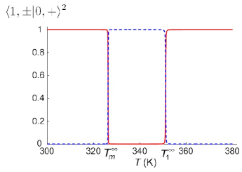
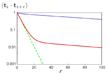
Figure 3: (a) Variation of the transition probabilities $\langle{1,\pm}|0,+\rangle^{2}$ with temperature (red solid line for $+$ and dashed blue line for $-$). For $T<T_{1}^{\infty}$, $\langle{1,+}|0,+\rangle^{2}\simeq\varphi_{U,\infty}$ and $\langle{1,-}|0,+\rangle^{2}\simeq\varphi_{B,\infty}$. One observes that for $T_{m}^{\infty}<T<T_{1}^{\infty}$, $\langle 1,-|0,+\rangle^{2}=1$ which underlines the relevance of $\xi_{1,-}^{p}$ in this temperature range (with parameter values $\tilde{\mu}=4.46$ kJ/mol, $\tilde{J}=9.13$ kJ/mol and $\tilde{K}=0$, see section VII). (b) Tangent-tangent correlation function given by Eq. (104) ($N,i\to\infty$) for 3 different temperatures: just before the transition (dotted blue line), controlled by $\xi_{1,+}^{p}\simeq\left[1/\xi_{U}^{p}+1/\xi_{I}\right]^{-1}\simeq\xi_{U}^{p}$; slightly above $T_{m}^{\infty}$ (solid red line), where the correlation length $\xi_{1,-}^{p}\simeq\xi_{B}^{p}$ is dominant for $r<r^{*}\simeq 20$; and after the transition ($T_{m}^{\infty}<T<T_{1}^{\infty}$) where the correlation length $\xi_{1,+}^{p}\simeq\xi_{I}$ disappears in favor of $\xi_{1,-}^{p}\simeq\xi_{B}^{p}$ (dashed green line).

Indeed, due to the coupling between bending and internal states of DNA, for realistic parameter values (cf. Section VII), the respective weights $\langle 0,+|1,\pm\rangle^{2}$ associated with each correlation length change abruptly at $T_{m}^{\infty}$: below $T_{m}^{\infty}$, we have $\langle 0,+|1,+\rangle\simeq\langle U|U\rangle=1$ and $\langle 0,+|1,-\rangle\simeq\langle U|B\rangle=0$, thus $\xi_{1,+}^{p}\simeq\xi_{U}^{p}$. For $T_{m}^{\infty}<T<T_{1}^{\infty}$, we find $\langle 0,+|1,+\rangle\simeq\langle B|U\rangle=0$ and $\langle 0,+|1,-\rangle\simeq\langle B|B\rangle=1$ which implies $\xi_{1,-}^{p}\simeq\xi_{B}^{p}$. For higher temperatures, $T>T_{1}^{\infty}$, the respective weights get swapped again, but now $\xi_{1,+}^{p}\simeq\xi_{1,-}^{p}$. These considerations lead us to introduce a critical distance, $r^{*}$, at which the two terms in Eq. (104) are equal:

$$r^{*}\equiv\left(\frac{1}{\xi_{1,-}^{p}}-\frac{1}{\xi_{1,+}^{p}}\right)^{-1}\ln\left(\frac{\langle 1,+|0,+\rangle^{2}}{\langle 1,-|0,+\rangle^{2}}\right)\simeq\xi_{B}^{p}\ln\left(\frac{\varphi_{B,\infty}}{\varphi_{U,\infty}}\right),$$ (111)

where in arriving at the last approximation we have used limiting forms that are valid when $T<T_{1}^{\infty}$ and assumed that $\xi_{B}^{p}\ll\xi_{U}^{p},\xi_{I}$ (cf. Fig. 4). When $r<r^{*}$ then the correlation function Eq. (104) is dominated by the shortest persistence length, $\xi_{1,-}^{p}$, and when $r>r^{*}$ the correlation function is dominated by the longest one, $\xi_{1,+}^{p}$. For sufficiently long chains and temperatures close enough to $T_{m}$, the inequality $N\gg r^{*}$ holds and this cross over should be clearly visible (see Fig. 3).

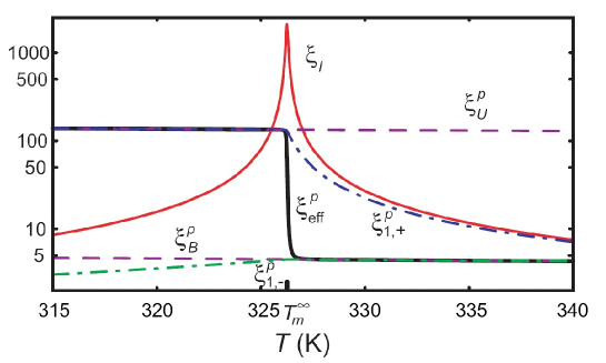
Figure 4: Variation with temperature of the various correlation lengths appearing in the model results: the Ising correlation length, $\xi_{I}$ (solid red line); persistence lengths of the coupled system, $\xi^{p}_{\rm eff}$ (appearing for long chains) and $\xi_{1,\pm}^{p}$ (dashed dotted line respectively blue and green); and of the pure chains, $\xi^{p}_{U,B}$ (dashed purple lines) (in units of $a$). At $T_{m}^{\infty}$, the Ising correlation length is peaked but finite, which is related to the point of closest approach of the two $(0,\pm)$ branches (zoom of Figure 2), and the effective persistence length, $\xi^{p}_{\rm eff}$, rapidly crosses over from $\xi^{p}_{U}$ to $\xi^{p}_{B}$ (parameter values $\tilde{\mu}=4.46$ kJ/mol, $\tilde{J}=9.13$ kJ/mol and $\tilde{K}=0$).

VI Mean-Square end-to-end distance

To calculate the mean-square end-to-end distance of the chain, we use the two-point correlation function obtained above:

$$\left(\frac{R}{a}\right)^{2}=\sum_{i,j=1}^{N}\langle{{\bf{t}}_{i}\cdot{\bf{t}}_{j}}\rangle=N+2\sum_{i=1}^{N-1}\sum_{r=1}^{N-i}\langle{\bf{t}}_{i}\cdot{\bf{t}}_{i+r}\rangle.$$ (112)

When all the bending rigidities are equal to $\kappa$, we recover, as expected, the pure discrete wormlike chain result:

$$R^{2}(\kappa)=a^{2}\,N\,W_{N}(u(\kappa))\,\,\mathrm{where}\,\,W_{N}(z)=\frac{1+z}{1-z}-\frac{2z}{N}\frac{1-z^{N}}{(1-z)^{2}}$$ (113)

with $u(\kappa)$ defined in Eq.(35). In the limit $N\to\infty$,

$$R^{2}(\kappa)\underset{N\to\infty}{\to}a^{2}\,N\,\frac{1+e^{-1/\xi_{p}(\kappa)}}{1-e^{-1/\xi_{p}(\kappa)}}.$$ (114)

More specifically, three distinct regimes can be identified:

$$R^{2}(\kappa)\to\left\{\begin{array}[]{*{20}c}a^{2}\,N,\\ 2\,a^{2}\,N\,\xi_{p}(\kappa),\\ a^{2}\,N^{2},\\ \end{array}\begin{array}[]{*{20}c}\xi_{p}(\kappa)\ll 1\ll N\\ 1\ll\xi_{p}(\kappa)\ll N\\ 1<N\ll\xi_{p}(\kappa)\\ \end{array}\right.\begin{array}[]{*{20}c}{\rm(freely\quad jointed\quad Gaussian)}\\ {\rm(effective\quad spin\quad wave\quad Gaussian)}\\ {\rm(rigid)}.\\ \end{array}$$ (115)

Because $\xi_{p}(\kappa)=\xi_{p}(\beta\tilde{\kappa})$ is decreasing function of temperature, the pure DWLC will go from the rigid to the effective Gaussian to the freely jointed Gaussian regime as the temperature is raised.

For the coupled model the double summation in Eq.(112) can also be carried out and we find

$$\left(\frac{R}{a}\right)^{2}=N+2\frac{\sum_{\tau_{1},\tau_{2},\tau_{3}}C(\tau_{3},\tau_{2},\tau_{1})\,S_{N}(\lambda_{0,\tau_{3}},\lambda_{1,\tau_{2}},\lambda_{0,\tau_{1}})\left(\frac{\lambda_{0,\tau_{1}}}{\lambda_{0,+}}\right)^{N-1}}{\sum_{\tau}\left(\frac{\lambda_{0,\tau}}{\lambda_{0,+}}\right)^{N-1}\langle V|0,\tau\rangle^{2}},$$ (116)

where

$$S_{N}({x,y,z})=\left\{\begin{array}[]{*{20}c}N\frac{y}{x-y}-\frac{y}{x}\frac{1-(y/x)^{N}}{(1-y/x)^{2}},\,\,\mathrm{for}\,\,x=z\\ z^{1-N}\frac{T_{N}(y,z)-T_{N}(y,x)}{z-x},\,\,\mathrm{for}\,\,x\neq z\\ \end{array}\right.,$$ (117)

with $T_{N}(x,y)=y^{N}\frac{x/y-(x/y)^{N}}{1-x/y}$. In the limit $N\to\infty$ the above complicated expression for $R^{2}$ simplifies to an effective Gaussian form

$$R^{2}\underset{N\to\infty}{\to}2a^{2}N\xi^{p}_{\rm eff}\quad\mathrm{where}\quad\xi^{p}_{\rm eff}\equiv\frac{1}{2}\sum_{\tau}\langle 1,\tau|0,+\rangle^{2}\frac{1+e^{-1/\xi_{1,\tau}^{p}}}{1-e^{-1/\xi_{1,\tau}^{p}}}$$ (118)

is an effective ”long chain” persistence length. This expression can be also obtained by using the simplified $N,i\to\infty$ limiting form for $\langle{{\bf{t}}_{i}\cdot{\bf{t}}_{i+r}}\rangle$, Eq. (104), in the general formula for $(R/a)^{2}$, Eq. (112). It tends to a further limiting form when $\xi_{1,\pm}^{p}\gg 1$:

$$\xi^{p}_{\rm eff}\to\sum_{\tau}\langle 1,\tau|0,+\rangle^{2}\xi_{1,\tau}^{p}\simeq\left\{\begin{array}[]{ll}\varphi_{U,\infty}\xi^{p}_{U}+\varphi_{B,\infty}\xi^{p}_{B},&T<T_{m}^{\infty}\\ \varphi_{U,\infty}\left[1/\xi^{p}_{U}+1/\xi_{I}\right]^{-1}+\varphi_{B,\infty}\xi^{p}_{B},&T_{m}^{\infty}<T<T_{1}^{\infty}\\ \end{array}\right.$$ (119)

At $T_{m}^{\infty}$ this expression simplifies reduces to $\xi^{p}_{\rm eff}\simeq\left(\xi_{U}^{p}+\xi_{B}^{p}\right)/2$ when $\xi_{I}\gg\xi^{p}_{U}$, which is actually the case (Fig. 4).

For $T<T_{m}^{\infty}$, the longest persistence length dominates: $\xi^{p}_{\rm eff}\simeq\xi_{1,+}^{p}\simeq\xi_{U}^{p}$. Above $T_{m}^{\infty}$, however, we see once again that there may be a competition between the persistence lengths, $\xi_{1,\pm}^{p}$, and the “transition probabilities”, ${\langle{1,\pm}|{0,+}\rangle}^{2}$, appearing in Eq. (119). This competition occurs now for $T>T_{m}^{\infty}$, contrary to what was found for the short distance behavior of the 2-point correlation function, Eq. (106), because the persistence lengths themselves appear in Eq. (119), and not their inverses. For $T_{m}^{\infty}<T<T_{1}^{\infty}$, depending on the weights, the smaller persistence length, $\xi_{1,-}^{p}$, may actually be dominant over the larger one, $\xi_{1,+}^{p}$; if so, $\xi^{p}_{\rm eff}\simeq\xi_{1,-}^{p}\simeq\xi_{B}^{p}$, which is actually the case when we consider standard parameter values for dsDNA and ssDNA (section VII), as shown in Fig. 4.

VII Application to synthetic DNA thermal denaturation

Melting or thermal denaturation profiles are experimentally obtained by following the UV absorbance of a DNA solution while slowly increasing the sample temperature. This method allows one to follow the temperature evolution of the fraction of base-pairs that have been disrupted, $\varphi_{B}(T)$. A typical profile has a sigmoid shape possibly with bumps that could appear depending on the DNA sequence. Different Ising-type models have been proposed wartmont ; wartben ; polscher ; gotoh for modeling denaturation curves by focusing on the influence of the base pair sequence, but they do not attempt to take into account properly the fluctuations of the DNA chains themselves. Yet, chain fluctuations increase with $T$ and play a crucial role in determining melting profiles. Moreover, these fluctuations concern both stiff helical segments and flexible coils with different bending rigidities.

In this section, we compare the model developed above, whose key element is to account for internal state fluctuations on an equal footing with those of the chain, with a set of experimental data. We focus on the evolution of $\varphi_{B}(T)$ for a synthetic homopolynucleotide polydA-polydT. Six independent parameters appear in the theory: the polymerization index $N$, the three Ising parameters $K$, $J$ and $\mu$ defined in Eq. (1) and Fig. 1, and bending moduli $\kappa_{U}$ for dsDNA and $\kappa_{B}$ for ssDNA. Note that we have also introduced a bending rigidity $\kappa_{UB}$ for domain walls. However $\kappa_{UB}$ appears in the theory only in the effective cooperativity parameter $J_{0}$. Thus changing $\kappa_{UB}$ is equivalent to varying the bare $J$, i.e. the energetic penalty to create a wall. Without any lost of generality, we choose to fix $\kappa_{UB}=\kappa_{U}$. Moreover, we choose free boundary conditions for the end monomers, which is valid unless their state is fixed by the experimental conditions libch (although any type of boundary conditions can be treated using our model). Of the six parameters, three are determined experimentally: $N$, $\kappa_{U}$, and $\kappa_{B}$. Moreover, there is evidence that stacking interactions in dsDNA and ssDNA are of the same magnitude which justifies the choice of $\tilde{K}=0$ adopted below goddard .

Figure 5 shows $\varphi_{B}(T)$ for a polydA-polydT of molecular weight $M_{w}=1180$ kDa in a solution of 0.1 SSC (0.015 M NaCl + 0.0015 M sodium citrate, pH 7.0) taken from wartmont .

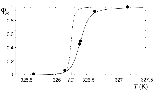
Figure 5: Fraction of broken base-pairs for a polydA-polydT vs. temperature (solution of 0.1 SSC, $N=1815$). The solid line represents the theoretical law for $\mu=1.64\,k_{B}T_{m}$ and $J=3.35\,k_{B}T_{m}$ where $T_{m}=326.4$ K. The case $N\to\infty$ for the same parameter values corresponds to the broken line.

In order to compare the data with our model predictions, we choose the experimental values persistence lengths, $\ell_{ds}^{p}\simeq 50$ nm and $\ell_{ss}^{p}\simeq 1$ nm at 300 K, which lead to $\kappa_{U}=\ell_{ds}^{p}/a=147$ and $\kappa_{B}=2\ell_{ss}^{p}/a=5.54$ at $T=T_{m}$ (taking $a=0.34$ nm for one base-pair size and a factor of 2 for two flexible segments in parallel per coil segment). The two remaining parameters $\tilde{\mu}$ and $\tilde{J}$ are determined by fitting the experimental data. The solid line in Fig. 5 corresponds to $\tilde{\mu}=1.64\,k_{B}T_{m}\simeq 4.46$ kJ/mol and $\tilde{J}=3.35\,k_{B}T_{m}\simeq 9.13$ kJ/mol leading to $T_{m}=326.4$ K. We can then deduce several thermodynamical features. Noting that the bare enthalpy for creating one A-T link is, in our model, $2\tilde{\mu}$, we find a value very close to the experimental value of 10.5 kJ/mol pincet . Although the value of $\tilde{J}$ is more difficult to interpret, our result $\tilde{J}\sim 2\tilde{\mu}$ is consistent with the idea that stacking interactions make the dominant contribution to DNA stability gotoh . Chain fluctuations do not only renormalize the effective free energy, $2\tilde{L}_{0}$, required to break an interior base-pair, but also the cooperativity parameter $\tilde{J}_{0}$: the latter varies almost linearly with $T$ following Eq. (17) contrary to previous theories where $\tilde{J}$ was taken as constant and supposed to be purely enthalpic in character wartmont . We have for the total cooperativity parameter $\tilde{J}_{0}=4.17\,k_{B}T_{m}$ at $T=T_{m}$, which shows that the bending contribution is roughly 25% (remembering that we have chosen $\kappa_{UB}=\kappa_{U}$). The model fit thus leads to parameter values in accord with experiment. Our model predictions for experimentally accessible A-T pair quantities are also in agreement with accepted values krueger ; metzler2 : i) the loop initiation, factor, $\sigma_{\rm LI}\equiv e^{-4J_{0}}\simeq 10^{-7}$ at $T_{m}$; and at physiological temperature, $T_{\rm ph}$, ii)  an interior single base-pair opening probability $\varphi_{B}(T_{\rm ph})\simeq 10^{-6}$ with a bubble initiation barrier of $17k_{B}T$ , and iii) a free energy of $0.18k_{B}T$ for breaking an additional base-pair in an already existing bubble. In reality, the fitted values of $\tilde{\mu}$ and $\tilde{J}$ implicitly compensate for effects like loop entropy explicitly left out of the model wartmont . As shown in Fig. 9 of wartmont , effective Ising models without loop entropy, like ours, can be considered to account implicitly (and approximately) for loop entropy, provided that one allows for loop entropy contributions to both $J$ and $K$. This loop entropy renormalization of the Ising model parameters will depend on the value of the loop entropy exponent $k$ and the chain length $N$ and could allow for a simple approximate way of accounting for the influence of loop entropy within the framework of an effective Ising model (cf. blossey ). This renormalization probably explains why our the model value for $\sigma_{\rm LI}$ is at the low end of the accepted spectrum.

In Fig. 5, the curve corresponding to the thermodynamic limit ($N\to\infty$) is shown for the same parameter values. In this case, $\varphi_{B}(T)$ is given by Eq. (56) and the value of the melting temperature is obtained analytically as a function of $T_{m}^{\infty}$ using $L_{0}(T_{m}^{\infty})=0$ which is given in the limit of low temperature ($\tilde{\kappa}_{B}\gg k_{B}T$) by

$$k_{B}T_{m}^{\infty}\simeq 2\frac{\tilde{\mu}+\tilde{K}}{\ln({\tilde{\kappa}}_{U}/{\tilde{\kappa}}_{B})}$$ (120)

Hence, the melting temperature is reached when the enthalpy required to create a link is perfectly balanced by the difference in (entropy dominated) free energy between the two types of semi-flexible chains (U or B). Another quantity which has an experimental relevance is the width of the transition. In the thermodynamic limit this width is narrow, but nonzero, due to the large but finite cooperativity parameter: $\Delta T_{m}^{\infty}\propto 1/\xi_{I}(T_{m}^{\infty})\simeq 2\exp[-2J_{0}(T_{m}^{\infty})]$ [see Eq. (57)]. Hence, the thermodynamic limit clarifies the role of the two free model parameters: in conjunction with the experimentally known bending rigidities, $\mu$ sets the melting temperature and $J$ fixes the transition width. This is in contrast to previous Ising-like models, where three fitting parameters were used $J$, $\partial L_{0}/\partial T$, and $T_{m}^{\infty}$ with $L_{0}$ assumed to by a linear function of $T$ wartmont .

Within the scope of our model the measured transition width is indicative of a very long Ising correlation length, $\xi_{I}$, near the transition temperature, much larger than the pure U and B persistence lengths; therefore typical helix (U) and bubble (B) domains (of size $\sim\xi_{I}$) are flexible within a small temperature window near the transition.

Included in the predictions of our theory are mechanical and structural features of the composed chain, such as persistence length or mean square end-to-end radius, $R$. This differs from purely Ising-type models wartmont ; gotoh and non-linear microscopic models peyrard ; dauxois where only thermodynamical quantities related to base-pairing are available. The variation of the effective persistence length $\xi^{p}_{\rm eff}$ (and thus the radius of gyration for long chains) vs. $T$ is shown in Fig. 4. It varies from $\xi^{p}_{U}$ for $T<T_{m}^{\infty}$ to $\xi^{p}_{B}$ for $T>T_{m}^{\infty}$. Since the transition is very abrupt, we suggest that the denaturation transition can also be followed experimentally by measuring directly the radius of gyration, for instance by tethered particle motion pouget , light scattering, or viscosity experiments. For instance, since the relative viscosity is proportional to $c_{\rm DNA}R^{3}$ (where $c_{\rm DNA}$ is the DNA concentration), it should clearly exhibit an abrupt thermal transition at a given $c_{\rm DNA}$ and $N$. Such a transition has indeed been observed for the viscosity of synthetic homopolynucleotide solutions inman , in qualitative agreement with Fig. 4.

In fitting our model to experiment for chains of length $N=1815$, we have found that finite size effects play an important role (Fig. 5). In the following section, we investigate such effects in detail.

VIII Finite size effects

It has been shown experimentally that DNA thermal denaturation varies with chain length, $N$ blake . In this section, we carefully study the effect of chain ends on the denaturation transition. In Fig. 6 are shown denaturation profiles for various chain lengths from $N=100$ to $N\to\infty$ and the fixed parameters values $\tilde{\mu}=4.46$ kJ/mol, $\tilde{J}=9.13$ kJ/mol and $\tilde{K}=0$ used in the previous section to fit the melting data. Within the scope of our model one observes that i) the melting temperature $T_{m}(N)$ is a decreasing function of $N$, varying as $[T_{m}(N)-T_{m}^{\infty}]/T_{m}^{\infty}\simeq 1/(N-1)$; ii) all the denaturation curves intersect at a temperature $T^{*}$ at which $\varphi_{B}\simeq 0.03$; iii) the transition width $\Delta T_{m}(N)$ is a decreasing function of $N$.

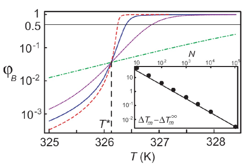
Figure 6: Linear-Log plot of melting curves for $N=100$ (dashed dotted green line), 500 (dotted purple line), 1815 (solid blue line), $\infty$ (dashed red line) in decreasing order at low temperature, $T<326$ K (parameter values $\tilde{\mu}=4.46$ kJ/mol, $\tilde{J}=9.13$ kJ/mol and $\tilde{K}=0$). We note that all the curves intersect at $T^{*}$, as discussed in the text. $T_{m}$ is defined by $\varphi_{B}=0.5$. Inset: Log-Log plot of model results for the shift in transition width $\Delta T_{m}-\Delta T_{m}^{\infty}$ vs. polymer length. Dots correspond to the model results and the solid line is a law in $1/N$.

Concerning points (i) and (ii), the observed behavior for the coupled system with the present parameter values is directly related to the model result that $T^{*}<T_{m}^{\infty}$, which is radically different from the behavior found for the simple Ising model (for which melting curves, $\varphi_{B}$, are strictly decreasing functions of $N$, because formally, $T^{*}=\infty$ when $\kappa_{U}=\kappa_{B}=\kappa_{UB}$). The present behavior for melting maps is also very different from the predictions of older empirical Ising-like models of denaturation and Helix-Coil like transitions nelson , for which the chemical potential $\mu$ appearing in the end vector $|V\rangle$ is incorrectly identified with $L_{0}$. This identification results in melting curves independent of $N$, i.e., $T_{m}=T^{*}$.

Concerning point (iii), the transition width roughly follows the law $(\Delta T_{m}-\Delta T_{m}^{\infty})\sim 1/(N-1)$, which is a classical result for finite size systems where fluctuations decrease in the thermodynamic limit. One observes that even for a long polymer, $N\sim 10^{3}$, finite size effects are important. For very short chains, e.g., $N<100$, such effects get amplified and we predict a transition width as large as $50$ K for $N=10$. This point is crucial, since it has been observed experimentally that for polydA-polydT inserts between more stable G-C rich domains, melting curves are much wider for very short DNA chains ($N\sim 10$ bp) libch with a width that decreases with increasing $N$ (observed for $60<N<140$ in blake ). In such experiments, the nature of end monomers clearly becomes extremely important.

For a given $N$ and $T$ the local site dependent bubble opening probability, or melting map,

$$\varphi_{B,i}=\frac{1-\langle\sigma_{i}\rangle}{2},$$ (121)

can be obtained from $\langle\sigma_{i}\rangle$ given in Eq. (65). In Fig. 7 $\varphi_{B,i}$ is plotted for six different temperatures using the same model parameter values employed in Fig. 5; we observe that below $T^{*}$ the chain unwinds from the ends, whereas above this temperature an interior bond has a higher probability of being open than an end one. Far enough below $T^{*}$ the melting curve heals rapidly to a plateau value close to $\varphi_{B,\infty}$ on a length scale on the order of $\xi_{I}\ll N$. At physiological temperature, $310$ K, the interior bond opening probability is $\simeq 10^{-6}$ in agreement with the experimental value for long runs of A-T pairs (which is an order of magnitude lower than randomly placed A-T pairs) krueger . At this temperature the end bonds have opening probabilities two orders of magnitude greater than the interior ones.

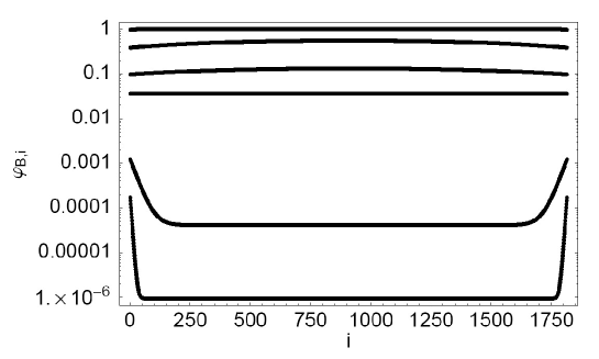
Figure 7: Average melting maps for different temperatures for $N=1815$ and the same parameter values used in Fig. 5: plot of the fraction of broken bases, $\varphi_{B,i}$ as a function of the base position $i$ for, in increasing order, 310 K, $0.99\,T^{*}=322.87$ K, $T^{*}=326.13$ K, $T_{m}^{\infty}=326.24$ K, $T_{m}=326.4$ K and $1.01\,T_{m}=329.66$ K.

At $T^{*}$ the melting curve is perfectly flat. This result, which is independent of chain length $N$, indicates that each Ising variable can be considered to fluctuate independently: $\langle\sigma_{i}\rangle$ is constant independent of $i$, despite a 2-point correlation function that does not factorize [$\langle\sigma_{i}\sigma_{i+r}\rangle\neq\langle\sigma_{i}\rangle\langle\sigma_{i+r}\rangle$, cf. Eq. (75)] and a large Ising correlation length ($\xi_{I}\gg 1$, see Fig. 4). Indeed, the influence of the renormalized stacking energy ($\sim\tilde{K}_{0}<0$), which favors bubble formation, exactly compensates that due to the renormalized destacking ($\sim\tilde{J}_{0}$), which suppresses bubble formation, and therefore $\varphi_{B,i}(T^{*})=[1-\tanh(\tilde{\mu}/(k_{B}T^{*})]/2\simeq 0.03$, which results from taking $N=1$ or taking $K_{0}=J_{0}=0$ for arbitrary $N$. In some ways this compensation leads to an effective non-interacting Ising system with $(\partial\langle c\rangle/\partial N)_{T^{*}}=(\partial\varphi_{B}/\partial N)_{T^{*}}=0$, which explains why the melting curves for different values of $N$ cross at $T^{*}$ in Fig. 6. Below $T^{*}$ the combined effects of the renormalized stacking energy and entropy gain favoring interior bubbles are too small to overcome the destacking energy cost associated with an extra domain wall and the chain ends unwind first. Since $K_{0}$ becomes more negative with increasing $T$ faster than $J_{0}$ increases, a temperature $T^{*}$ is reached where the renormalized stacking and destacking effects just compensate. Above $T^{*}$ the situation is reversed and the opening probability is higher in the chain interior. For arbitrary $N$ and $T$, the thermodynamic chemical potential, defined by $\hat{\mu}=(\partial F/\partial N)_{T}$ can be related to $\langle c\rangle$ via Maxwell-type relations, leading to $(\partial\hat{\mu}/\partial\tilde{\mu})_{T,N}=N(\partial\langle c\rangle/\partial N)_{T}-\langle c\rangle$. At $T^{*}$ this general relation simplifies to $(\partial\hat{\mu}/\partial\tilde{\mu})_{T^{*},N}=-\langle c\rangle|_{T^{*}}=(\partial f/\partial\tilde{\mu})_{T^{*},N}$, characteristic of a non-interacting system.

Upon examination of Eqs. (65) and (90), we see that $T^{*}$ is determined by the condition that $\left\langle{\sigma_{i}}\right\rangle=\langle c\rangle_{\infty}$, which is obtained when the end vector $|V\rangle$ is identical to the eigenket $|0,+\rangle$ and orthogonal to $|0,-\rangle$: $\langle V|0,+\rangle=1$ and $\langle V|0,-\rangle=0$. Physically, this means that the coupled Ising-chain system is in a pure state, $|0,+\rangle$, that mixes the canonical states in a special way. The temperature $T^{*}$ can be obtained by solving $\langle V|0,-\rangle=0$. Using Eqs. (11) and (43)-(44) this translates into $e^{\mu}=e^{-2J_{0}}\{\sinh(L_{0})+[\sinh^{2}(L_{0})+e^{-4J_{0}}]^{1/2}\}$. After some manipulation using Eq. (56), this can be shown to be identical to $\langle c\rangle_{\infty}(T^{*})=\langle c\rangle(N=1,T^{*})=\tanh[\tilde{\mu}/(k_{B}T^{*})]$. Furthermore, Eqs. (66) and (98) show that the Ising and chain 2-point correlation functions, $\langle{\sigma}_{i}\cdot{\sigma}_{i+r}\rangle$ and $\langle{\bf t}_{i}\cdot{\bf t}_{i+r}\rangle$, also get simplified at $T^{*}$: the approximate forms, Eqs. (75) and (104) valid in general only for $N,i\rightarrow\infty$, become exact for arbitrary $N$ and $i$ at this special temperature. It is clear that at $T^{*}$ the coupled system behaves as if there are no end effects and finite chains have the same behavior as an infinite one.

To shed additional light on this mechanism and illustrate the important role of internal bubble entropy for long chains, we now study an infinite chain and compare $\varphi_{B,{\rm int}}=\lim_{N,i\rightarrow\infty}\varphi_{B,i}$ with $\varphi_{B,{\rm end}}=\lim_{N\rightarrow\infty}\varphi_{B,1}$. Equation (71) shows that $\xi_{I}$ plays here the role of a healing length, over which end effects relax (see Fig. 7). The ratio of matrix elements appearing in Eq. (71) gets simplified in the following way for special values of $T$:

$$R_{V}=\frac{\langle V|0,-\rangle}{\langle V|0,+\rangle}=\left\{\begin{array}[]{ll}-e^{-\mu},&T<T^{*}\\ 0,&T=T^{*}\\ \tanh(\mu/2),&T=T_{m}^{\infty}\\ e^{\mu},&T>T_{m}^{\infty}\\ \end{array}\right.$$ (122)

At $T_{m}^{\infty}$, Eq. (71) simplifies to

$$\left\langle{\sigma_{i}}\right\rangle_{\infty}(T_{m}^{\infty})=\tanh\left(\frac{\tilde{\mu}}{2k_{B}T_{m}^{\infty}}\right)\exp[-(i-1)/\xi_{I}(T_{m}^{\infty})],$$ (123)

which shows that for very long chains ($N\gg\xi_{I}$) at $T_{m}^{\infty}(>T^{*})$ $\varphi_{B,{\rm end}}=[1-\tanh[\tilde{\mu}/(2k_{B}T_{m}^{\infty})]/2\simeq 0.16\ll\varphi_{B,\infty}(T_{m}^{\infty})=1/2$, revealing an internal opening probability more than three times higher than an end one. In Figs. 7 and 8, however, we observe that for $T=T_{m}$ and $T_{m}^{\infty}$, $\xi_{I}>N=1815$ (cf. Fig. 4), and therefore end effects do not get damped out near the center of this finite chain. Indeed, at $T_{m}^{\infty}$ the opening probability $\varphi_{B,i}$ near the middle of a chain of length $N=1815$ is much less than the value of 1/2 holding for an infinite one. For $N=1815$ we still observe, however, noticeable differences ($\sim 10$ to 20%) between interior and end opening probabilities near $T_{m}$.

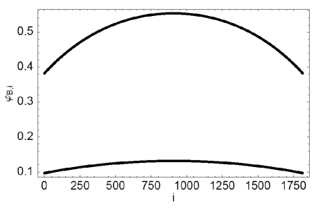
Figure 8: Zoom of the melting map shown in Fig. 7 for $T_{m}^{\infty}$ (lower curve) and $T_{m}$ (upper curve).

The one-sequence-approximation has been defined by Poland and Scheraga polscher and consists in neglecting the many small bubbles which eventually collapse and considering only one large thermally excited bubble. It is valid for temperatures sufficiently far below $T_{m}^{\infty}$. For $N\to\infty$, $\varphi_{B,{\rm int}}$ and $\varphi_{B,{\rm end}}$ can be estimated in this approximation by summing over, respectively, all the interior and end bubbles containing the fixed site in question. In the interior case we thus have

$$\varphi_{B,{\rm int}}\simeq\sum_{n=1}^{\infty}n\exp\left[-\beta\Delta G_{\rm int}^{(n)}\right]=e^{-4J_{0}}\sum_{n=1}^{\infty}n\;e^{-2nL_{0}}=\frac{e^{-4J_{0}}}{4\sinh^{2}(L_{0})}.$$ (124)

The factor of $n$ in the sum is entropic in nature and equal to the number of ways of placing a fixed interior site within an interior $n$-bubble. In the end case, where there is no entropic factor,

$$\varphi_{B,{\rm end}}\simeq\sum_{n=1}^{\infty}\exp\left[-\beta\Delta G_{\rm end}^{(n)}\right]=e^{K_{0}-2J_{0}}\sum_{n=1}^{\infty}e^{-2nL_{0}}=\frac{e^{-(2J_{0}+\mu)}}{2\sinh(L_{0})}.$$ (125)

It is important to note that for the model parameters employed, the additional dimensionless free energy for breaking an additional base-pair in an already existing bubble, $2L_{0}\simeq 0.18$ at physiological temperature, is less than one and much smaller than the bubble initiation energy cost for an end bubble, $\sim 2J_{0}\simeq 8$ (and a fortiori for an interior one, $\sim 4J_{0}$). This implies that even at physiological temperature, where the probability of bond opening is very small, bubbles covering a wide range of sizes contribute to the sums in Eqs. (124)-(125): both $\langle n\rangle_{\rm int}=\coth(L_{0})\simeq 1/L_{0}\simeq 6$ and $\langle n\rangle_{\rm end}=e^{-L_{0}}/[2\sinh(L_{0})]\simeq 1/(2|L_{0}|)\simeq 3$ are of the same order of magnitude as $\xi_{I}$, which varies as $1/(2|L_{0}|)$ when $|L_{0}|\ll 1$. Because $L_{0}$ decreases with $T$ (going to 0 at $T_{m}^{\infty}$), both $\varphi_{B,{\rm int}}$ and $\varphi_{B,{\rm end}}$ are increasing functions of temperature. For $T<T^{*}$ the bubble initiation energy cost dominates and $\varphi_{B,{\rm int}}<\varphi_{B,{\rm end}}$. Thanks to the entropic factor, however, $\varphi_{B,{\rm int}}$ increases more rapidly than $\varphi_{B,{\rm end}}$ and the two curves cross over at $T^{*}$, an estimate of which can be obtained by equating the above two one-sequence-approximations for both these quantities. As a check on the preceding discussion, the one-sequence-approximations for infinite chains obtained above for end and interior opening probabilities can be shown to be in exact agreement with what one gets from the definition of $\varphi_{B,i}$, Eq. (121), and Eq. (71) by using the low temperature approximations for $\langle V|0,-\rangle/\langle V|0,+\rangle\simeq-e^{-\mu}$ [Eq. (122)] and $\langle c\rangle_{\infty}$, Eq. (56), i.e. expanding to lowest order in $e^{-4J_{0}}$, assuming that $e^{-4J_{0}}\ll\sinh^{2}(L_{0})$, which is the formal criterion for the validity of the one-sequence-approximation.

Using the one-sequence-approximation, it is now easy to see how the cost in loop entropy associated with internal bubbles will modify the above results. In the so-called loop entropy models wartmont ; polscher ; polscher the internal bubbles formed by the single strands are visualized as one polymer loop, whose entropic cost has been estimated first by Zimm zimm . Hence, although $\varphi_{B,{\rm end}}$ does not change, the interior opening probability does, becoming

$$\varphi_{B,{\rm int}}^{\rm LE}\simeq\sum_{n=1}^{\infty}n/(n_{0}+n)^{k}\exp[-\beta\Delta G_{\rm int}^{(n)}],$$ (126)

where we have adopted a common simplified form for the loop entropy factor, $f_{\rm LE}(n)=(n_{0}+n)^{-k}$ parametrized by a constant $n_{0}$, which may be as large as 100 blake , and an exponent $k$, usually assumed to be in the range $3/2\leq k\leq 2.1$, depending on the extent to which chain self-avoidance is taken into account peliti . A large value for $n_{0}$ would severely reduce the importance of loop entropy for short chains and probably reflects the presence of strong bending rigidity effect (an important open question concerns how to incorporate bending rigidity into $f_{\rm LE}$ in a physically correct way). Loop entropy clearly lowers the probability of interior bubble opening and will lead to an increase in $T^{*}$. The situation is further complicated if strand sliding, which may be important for periodic DNA, is taken into account. For homopolymeric DNA like polydA-polydT, strand sliding leads to a modified loop entropy exponent, $k^{\prime}=k-1$ wartmont ; polscher ; orland2 , resulting in a significant decrease in the importance of loop entropy. By the way, it also minimizes the importance for homopolymeric DNA of recent claims that a true first-order phase transition should occur for infinite chains because $k$ appears to be greater than 2 when self-avoidance is fully taken into account peliti . The combined effects of loop entropy and strand sliding will lead to increases in both $T^{*}$ and $T_{m}^{\infty}$. Neither the theoretical nor the experimental situation concerning $T_{m}(N)$ is entirely clear for homopolymeric DNA with free ends and further careful experiments are clearly called for. If loop entropy and strand sliding are included in the coupled Ising-chain model, $T^{*}$ might become higher than $T_{m}^{\infty}$, which would imply that $T_{m}(N)$ would increase with $N$ polscher , unlike what what we find to occur when these two effects are neglected.

In the future, we intend to examine these questions by incorporating loop entropy and strand sliding directly into our DNA model. With all other factors being equal, adding loop entropy and strand sliding increases the stability of the closed state, resulting in sharper melting curves and higher values of $T_{m}(N)$ (see Figs. 9 and 10 of wartmont and blossey ). The importance of this loop entropy contribution would change with chain length $N$ and may lead to an increase in $T_{m}(N)$ with increasing $N$ polscher at least for a certain range of chain sizes .

IX Summary and Conclusion

This paper presents a novel theoretical model of DNA denaturation, already introduced in prl , which focuses on the coupling between the base-pair link state (unbroken or broken) and the rotational degrees of freedom of the semi-flexible chain. The Hamiltonian includes local chain bending rigidities whose values depend on neighboring base-pair states: around 5 $k_{B}T$ for bubbles and 150 $k_{B}T$ for connected base-pair segments. Because of the rotational symmetry, the model can be rewritten in terms of an effective Ising Hamiltonian by integrating out the rotational degrees of freedom of the chain. Hence, our model yields considerable insight into the empirical temperature-dependent parameters used in previous Ising-like models wartmont . In particular, the melting temperature $T_{m}$ is no longer a fitting parameter, but emerges naturally as a function of: (i) experimentally known bending rigidities, $\kappa_{U}$ and $\kappa_{B}$; (ii) the bare energy required to open a base-pair, $2\tilde{\mu}$; (iii) the bare energy of a domain wall, or destacking, $2\tilde{J}$; (iv) the difference in bare stacking energy between ss and dsDNA, $2\tilde{K}$; and (v) the polymerization index, $N$. Moreover, our model allows structural features of the DNA chain, such as the mean size $R$, to be calculated as a function of $T$. An abrupt transition for $R$ is found at $T_{m}$ and explains, at least qualitatively, the thermal transition observed in viscosity measurements inman .

From an experimental perspective, our results obtained from exactly solving the coupled model can be summarized as follows. First of all, we propose formulæ for chain free-boundary conditions, this information being encoded in the end vector $|V\rangle$ given in Eq. (11). However, any other boundary condition can be treated following the same route, even though we shall not detail the calculations here. For example, a polydA-polydT sequence of length $N$ sandwiched between more stable G-C sequences libch can be seen near its melting transition as a DNA of length $N$, with fixed boundary conditions, resulting in an end vector $|V\rangle=|U\rangle$.

Once boundary conditions are set, our model predicts melting profiles, as measured for example from UV absorbance experiments. Even if the model relies upon six microscopic parameters, as discussed in section VII, most of them are known experimentally, including the strand length $N$, and only two of them must be extracted from melting profiles: $\tilde{\mu}$, the bare half-energy required to break a base pair (which can also be estimated experimentally pincet ), and $\tilde{J}$, the cooperativity parameter that indicates the cost of creating a domain wall between unbroken and broken base pairs (recent experiments on single DNA molecules aim at determining this quantity, see ke ). Melting profiles, giving the fraction of broken base pairs, $\varphi_{B}$, as a function of the temperature $T$, are determined through the average of the Ising state variable, $\langle c\rangle$, because $\varphi_{B}(N,T)=[1-\langle c\rangle(N,T)]/2$.

For infinite chains, ($N\rightarrow\infty$), the expression for $\langle c\rangle_{\infty}(T)$ is rather simple (Eq. (56)):

$$\left\langle c\right\rangle_{\infty}(T)=\frac{\sinh(L_{0})}{[\sinh 2(L_{0})+e^{-4J_{0}}]^{1/2}},$$ (127)

where the renormalized parameters $J_{0}$, $K_{0}$, and $L_{0}=\mu+K_{0}$ are given in Eqs. (17), (18), and (23). In these latter equations, the function $G_{0}(\kappa)$ has a simple algebraic expression (Eq. (13)) that reduces to a purely entropic contribution, $G_{0}(\kappa)\simeq\ln(2\kappa)$, in the physically relevant low-$T$ (spin wave) approximation. From the melting profile $\varphi_{B,\infty}(T)$, the melting temperature, $T_{m}^{\infty}$, is defined by $\varphi_{B,\infty}=1/2$, in other words by $L_{0}=0$. The finite transition width is estimated by Eq. (57): $\Delta T_{m}^{\infty}\simeq 2\,k_{B}[T_{m}^{\infty}]^{2}\exp[-2\,J_{0}(T_{m}^{\infty})]/{\tilde{\mu}}$.

For finite length strands ($N$ finite), the expression for $\langle c\rangle(N,T)$, Eq. (68), is more complex, because $N$ has an influence on $\varphi_{B}(N,T)$ and thus $T_{m}$. In addition, the interplay with mechanisms, such as loop entropy, not taken into account in this study is nontrivial, as discussed in detail in section VIII. At the level tackled in the present paper, we obtain a simplified expression for $\langle c\rangle(N,T)$ when $N$ is large, Eq. (73), which simplifies even further when $N\gg\xi_{I}\gg 1$ (Fig. 7):

$$\langle c\rangle(N,T)\simeq\langle c\rangle_{\infty}+2R_{V}(\xi_{I}/N)\;(1-\langle c\rangle_{\infty}^{2})^{1/2},$$ (128)

where $R_{V}$, Eq. (69), which is a ratio of matrix elements pertaining to end effects, simplifies at certain special temperatures, see Eq. (122). Note that finite-size effects are still important for sizes of several thousands of base pairs (see sections VII and VIII and Figs 7 and 8) and are not a purely academic debate.

Three important correlation lengths can be calculated in the framework of our model. On the one hand, the Ising correlation length $\xi_{I}$, gives access to the typical size of bubbles in the low temperature regime ($T<T_{m}$), as well as to the typical size of unbound regions for $T>T_{m}$. This quantity is calculated in Eq. (70) and assumes a simplified form at $T_{m}^{\infty}$: $\xi_{I}(T_{m}^{\infty})\simeq\exp[2J_{0}(T_{m}^{\infty})]/2\gg 1$, when $J_{0}(T_{m}^{\infty})\gg 1$. On the other hand, one effective chain persistence length, $\xi^{p}_{\rm eff,CF}\simeq[\varphi_{U,\infty}/\xi_{U}^{p}+\varphi_{B,\infty}/\xi_{B}^{p}]^{-1}$, provides information on the short distant behavior of the chain tangent-tangent correlation function, Eq. (106), and the other, $\xi^{p}_{\rm eff}$, provides information on the typical chain conformations, in particular its mean-square-radius:

$$\langle{\bf R}^{2}\rangle\simeq 2a^{2}N\xi^{p}_{\rm eff}\simeq 2a^{2}N(\varphi_{U,\infty}\xi^{p}_{U}+\varphi_{B,\infty}\xi^{p}_{B}),$$ (129)

where $a$ is the monomer length (0.34 nm) and the approximation is valid for very long chains (large $N$). Knowing this quantity is of primary importance when interpreting data from Tethered Particle or Tweezer experiments pouget ; Smith92 ; pouget2 , Atomic Force Microscopy Wiggins06 or viscosity measurements inman . The results that we have obtained here for the chain tangent-tangent correlation function and mean-square-radius are very different from what one obtains by solving a quenched random rigidity model, where the local joint rigidity can take on one of two values, $\kappa_{1}$ and $\kappa_{2}$, with probability $\varphi_{1}$ and $\varphi_{2}=1-\varphi_{1}$. In this case there is only one effective correlation length: $\overline{\langle{\bf t}_{i}\cdot{\bf t}_{i+r}\rangle}=e^{-r/\xi^{p}_{\rm ran}}$ and $\overline{\langle{\bf R}^{2}\rangle}\simeq 2a^{2}N\xi^{p}_{\rm ran}$, where $\xi^{p}_{\rm ran}\equiv-1/\ln[\varphi_{1}e^{-1/\xi_{p}(\kappa_{1})}+\varphi_{2}e^{-1/\xi_{p}(\kappa_{2})}]$ and $\xi_{p}(\kappa)$ is given by Eq. (36).

The foregoing analysis makes allowance for neither solvent entropic (hydrophobic), nor electrostatic effects, which might not only change the actual value of the bare Ising parameters $\tilde{J}$, $\tilde{K}$ and $\tilde{\mu}$, but also lead to additional entropic contributions. To go further concerning solvent entropic effects would require molecular dynamics simulations, which is beyond the scope of the present approach. The electrostatic effects in DNA melting are two-fold: an entropic contribution arising from the difference in electrostatic energy between states $U$ and $B$ and an an enthalpic contribution arising from counterion release. At equilibrium the two effects partially compensate and the remaining contribution is, using a simple thermodynamic approach in the low salt limit manning2 ; korolev , approximately equal to $\Delta G_{\rm el}=k_{B}T\ell_{b}(\tau_{B}-\tau_{U})\ln(I/I_{0})$, where $I$ is the ionic strength ($I_{0}=1$  M), $\ell_{b}=e^{2}/(4\pi\epsilon k_{B}T)$ the Bjerrum length ($e$ is the elementary charge and $\epsilon$ the water dielectric permittivity) and $\tau_{U}$ and $\tau_{B}$ are the linear charge densities of the pure U and B chains, respectively. Although this is an approximate result and the determination of $\tau_{B}-\tau_{U}$ remains controversial, these two contributions should be included in a more refined model. A natural extension emerging from this study concerns the ionic strength dependence of DNA melting profiles and effective persistence lengths.

The current rapid development of force experiments in magnetic or optical tweezer traps Smith92 , “Tethered Particle Motion” experiments pouget or even more recently atomic force microscopy ones Wiggins06 , presents a formidable opportunity to investigate directly the elastic properties of DNA strands as a function of temperature, salt concentration and length $N$. Indeed, despite the pioneering work by Blake and Delcourt blake , a systematic experimental study of the effect of $N$ while controlling the nature of chain ends, is lacking, especially for homopolymers. This would be a way to discriminate between the different models and also shed light on the role of loop entropy, which is neglected in the present model.

The approach developed here can be extended to bubble dynamics. Very recent work metzler2 ; metzler1 ; mukamel studied the growth of already nucleated bubbles using the Fokker-Planck equation applied to the Poland-Scheraga model (i.e., an effective Ising model including loop entropy). The agreement with experimental results obtained by fluorescence correlation spectroscopy is remarkably good metzler2 . The issue of bubble nucleation is, however, not solved and will be continued to be explored in the near future. In addition the mutual influence of thermally excited bubbles and chain flexibility should play an important role in determining global DNA conformations and strongly influence looping dynamics pouget2 ; finzi .

Symbol	Quantity	Mathematical definition	Reference
$T_{m}$	melting temperature	$\varphi_{U}(T_{m})=\varphi_{B}(T_{m})=1/2$	Secs. I, II
$N$	chain length		Sec. II
${\rm U}/{\rm B}$	unbroken/broken base pair		Sec. II
$\varphi_{U,B}$	fractions of U’s and B’s		Eq. (6)
$\sigma_{i}$	internal degree of freedom (Ising variable)	$\pm 1$	Sec. II
${\bf{t}}_{i}$	chain unit tangent vector (Heisenberg variable)	$\|{\bf{t}}_{i}\|=1$	Sec. II
$\tilde{\kappa}_{i,i+1}$	local chain bending rigidity (coupling)	$\kappa_{U},\kappa_{B}$ or $\kappa_{UB}$	Sec. II
$\tilde{J}$	half-energy of a domain wall		Sec. II
$\tilde{K}$	difference in stacking energy between ds and ssDNA		Sec. II
$\tilde{\mu}$	half-energy required to open a base-pair		Sec. II
$\kappa,J,K,\mu,\ldots$	adimensional energies (in units of $k_{B}T$)	$\kappa=\beta\tilde{\kappa}$, …	Sec. II
$G_{0}(\kappa)$	free energy of a single joint of rigidity $\kappa$	$\kappa-\ln[\sinh(\kappa)/\kappa]$	Sec. II
$J_{0}$	renormalized (effective) Ising parameter $J$	$J-\frac{1}{4}[G_{0}(\kappa_{U})+G_{0}(\kappa_{B})-2G_{0}(\kappa_{UB})]$	Eq. (17)
$K_{0}$	renormalized (effective) Ising parameters $K$	$K-\frac{1}{2}[G_{0}(\kappa_{U})-G_{0}(\kappa_{B})]$	Eq. (18)
$L_{0}$	effective chemical potential to open an interior base pair	$\mu+K_{0}$	Sec. II
$\langle c\rangle_{\infty}$	infinite size Ising “magnetization”	$\sinh(L_{0})/[\sinh^{2}(L_{0})+e^{-4J_{0}}]^{1/2}$	Eq. (56)
$\varphi_{U,\infty}$, $\varphi_{B,\infty}$	fraction of unbroken (U) and broken (B) bonds ($N\to\infty$)	$[1\pm\langle c\rangle_{\infty}]/2$	Sec. III
$\varphi_{B,i}$	site $i$ bonding opening probability (melting map)	$[1-\langle\sigma_{i}\rangle]/2$	Eq. (121)
$T_{m}^{\infty}$	infinite size ($N\rightarrow\infty$) melting temperature	$L_{0}(T_{m}^{\infty})=0$	Sec. II
$\Delta T_{m}^{\infty}$	transition width ($N\rightarrow\infty$)	$2|\partial\langle c\rangle_{\infty}/\partial T|^{-1}$ at ${T_{m}^{\infty}}$ & Figs. 5 and 6	Eq. (57)
$\langle\sigma_{i+r}\sigma_{i}\rangle$	Ising correlation function		Sec. IV
$\xi_{I}$	Ising correlation length	$e^{2J_{0}}/2$ at ${T_{m}^{\infty}}$ & Fig. 4	Sec. IV
$\langle{\bf{t}}_{i+r}\cdot{\bf{t}}_{i}\rangle$	chain correlation function	Fig. 3(b)	Sec. V
$\xi^{p}_{1,+},\xi^{p}_{1,-}$	persistence lengths	Fig. 4	Eq. (104)
$\xi^{p}_{{\rm eff}}$	effective persistence length	Fig. 4	Sec. VI
$R$	chain mean square (or gyration) radius	$\langle{\bf R}^{2}\rangle^{1/2}$	Secs. II,VI
$T^{*}$	crossover temperature for finite chains	$\partial\varphi_{B}/\partial N|_{T^{*}}=0$	Sec. VIII

Table 1: Index of the main symbols used throughout the paper, with their mathematical definition, and reference.

References

- (1) J. SantaLucia Jr., Proc. Nat. Acad. Sci. USA 95 1460 (1998).
- (2) P. Pincet, E. Perez, G. Bryant, L. Lebeau, and C. Mioskowski, Phys. Rev. Lett. 73 2780 (1994).
- (3) A. Krueger, E. Protozanova and M.D. Frank-Kamenetskii, Biophys. J. 90, 3091 (2006).
- (4) R.M. Wartell and E.W. Montroll, Adv. Chem. Phys. 22 129 (1972).
- (5) O. Gotoh, Adv. Biophys. 16 1 (1983).
- (6) YU.S. Lazurkin, M.D. Frank-Kamanetskii, and E.N. Trifonov, Biopolymers 9 1253 (1970).
- (7) G. Kalosakas G. et al., Europhys. Lett. 68 127 (2004).
- (8) M.Th. Record, Jr., Ch.F. Anderson, and Lohman T.M., Q. Rev. Biophys. 11 103 (1978).
- (9) P. Nelson, Biological Physics. Energy, Information, Life., W.H. Freeman and Compagny, New York, 2004, Section 9.
- (10) R. D. Blake and S. G. Delcourt, Biopolymers. J. 26 2009 (1987).
- (11) J.B. Fiche, A. Buhot, R. Calemczuk, and T. Livache, Biophys. J. 92 935 (2007).
- (12) C.J. Benham, J. Mol. Biol. 255, 425 (1996); R.M. Fye and C.J. Benham, Phys. Rev. E 59, 3408 (1999).
- (13) R.M. Wartell and A.S. Benight, Physics Rep. 126 67 (1985).
- (14) D. Poland and H.R. Scheraga, Theory of Helix Coil Transition in Biopolymers, Academic Press, New York, 1970.
- (15) B.H. Zimm and Bragg J.K., J. Chem. Phys. 31 526 (1959); B.H. Zimm, J. Chem. Phys. 33 1349 (1960).
- (16) R.D. Blake et al., Bioinformatics 15, 370 (1999).
- (17) R. D. Blake and S. G. Delcourt, Nucleic Acids Res. 26 3323 (1998).
- (18) Y. Kafri, D. Mukamel and L. Peliti, Phys. Rev. Lett. 85, 4988 (2000).
- (19) E. Carlon et al., Phys. Rev. Lett. 88, 198101 (2002).
- (20) M. Peyrard and A.R. Bishop., Phys. Rev. Lett. 62, 2755 (1989).
- (21) T. Dauxois, M. Peyrard, and A.R. Bishop., Phys. Rev. E 47, 684 (1993).
- (22) D. Cule and T. Hwa, Phys. Rev. Lett. 79, 2375 (1997).
- (23) M. Peyrard, Nonlinearity 17, R1 (2004).
- (24) Y. Gao, K.V. Devi-Prasad and E.W. Prohovsky, J. Chem. Phys. 80, 6291 (1984).
- (25) J.-H. Jeon, W. Sung and F.H. Ree, J. Chem. Phys. 124, 164905 (2006).
- (26) T.E. Cheatham and P.A. Kollman, J. Mol. Biol. 259 434 (1996).
- (27) T. Garel, C. Monthus, and H. Orland, Europhys. Lett. 55 132 (2001).
- (28) J. Palmeri, M. Manghi, and N. Destainville, Phys. Rev. Lett. 99, 088103 (2007).
- (29) J. Yan and J.F. Marko, Phys. Rev. Lett. 93 108108 (2004).
- (30) J. Palmeri and S. Leibler, Dynamical Phenomena at Interfaces, Surfaces and Membranes, Eds. D. Beysens, N. Boccara and G. Forgacs, Nova Science Publishers, Inc., New York, 1993, 323.
- (31) C. Storm and P.C. Nelson, Europhys. Lett. 62 760 (2003).
- (32) M.E. Fisher, Am. J. Phys. 32 343 (1964).
- (33) G.S. Joyce, Phys. Rev. 155 478 (1967).
- (34) M. Grifoni and P. Hänggi, Phys. Rep. 304 229 (1998).
- (35) D. Chandler, Introduction to Modern Statistical Mechanics, Oxford University Press, New York, 1987, Section 5.8.
- (36) C. Cohen-Tannoudji, B. Diu and F. Laloë, Mécanique Quantique, Hermann, Paris, 1973, vol. 2.
- (37) G. Altan-Bonnet, A. Libchaber, and O. Krichevsky, Phys. Rev. Lett. 90 138101 (2003).
- (38) D.P. Aalberts, J.M. Parman and N.L. Goddard, Biophys. J. 84, 3212 (2003).
- (39) H. C. Fogedby and R. Metzler, Phys. Rev. Lett. 98, 070601 (2007).
- (40) R. Blossey and E. Carlon, Phys. Rev. E 68, 061911 (2003)
- (41) N. Pouget et al., Nucleic Acids Res. 32, e73 (2004).
- (42) R.B. Inman and R.L. Baldwin, J. Mol. Biol. 8, 452 (1964).
- (43) T. Garel and H. Orland, Biopolymers 75, 453 (2004).
- (44) C. Ke, M. Humeniuk, H. S. Gracz, and P. E. Marszalek, Phys. Rev. Lett. 99, 018302 (2007).
- (45) S.B. Smith, L. Finzi, and C. Bustamante, Science 258 1122 (1992).
- (46) N. Pouget et al., Nucleic Acids Res. 34, 4313 (2006).
- (47) P.A. Wiggins et al., Nature Nanotechnology 1 137 (2006).
- (48) G.S. Manning, Biopolymers 11 937 (1972).
- (49) N. Korolev, A.P. Lyubartsev, and L. Nordenskiöld, Biophys. J. 75 3041 (1998).
- (50) T. Ambjörnsson, S.K. Banik, O. Krichevsky, and R. Metzler, Phys. Rev. Lett. 97,128105 (2006).
- (51) A. Bar, Y. Kafri and D. Mukamel, Phys. Rev. Lett. 98, 038103 (2007).
- (52) L. Finzi and J. Gelles, Science 267, 378 (1995).