INSTITUT NATIONAL DE RECHERCHE EN INFORMATIQUE ET EN AUTOMATIQUE

Triangulating the Real Projective Plane
Mridul Aanjaneya — Monique Teillaud N° 6296
Septembre 2007

Abstract: We consider the problem of computing a triangulation of the real projective plane $\mathbb{P}^{2}$, given a finite point set $\mathcal{P}=\{p_{1},p_{2},\ldots,p_{n}\}$ as input. We prove that a triangulation of $\mathbb{P}^{2}$ always exists if at least six points in $\mathcal{P}$ are in general position, i.e., no three of them are collinear. We also design an algorithm for triangulating $\mathbb{P}^{2}$ if this necessary condition holds. As far as we know, this is the first computational result on the real projective plane.

Key-words: Computational geometry, triangulation, simplicial complex, projective geometry, algorithm

Trianguler le plan projectif réel

Résumé : Nous considérons le calcul de la triangulation d’un ensemble fini de points $\mathcal{P}=\{p_{1},p_{2},\ldots,p_{n}\}$ dans le plan projectif. Nous démontrons que la triangulation existe toujours dès lors qu’au moins six points de $\mathcal{P}$ sont en position générale, c’est-à-dire que trois d’entre eux ne sont jamais alignés. Nous proposons également un algorithme pour trianguler $\mathbb{P}^{2}$ si cette condition nécessaire est remplie. À notre connaissance, c’est le premier résultat algorithmique connu pour le plan projectif réel.

Mots-clés : Géométrie algorithmique, triangulation, complexe simplicial, géométrie projective, algorithme

1 Introduction

The real projective plane $\mathbb{P}^{2}$ is in one-to-one correspondence with the set of lines of the vector space $\mathbb{R}^{3}$. Formally, $\mathbb{P}^{2}$ is the quotient $\mathbb{P}^{2}=\mathbb{R}^{3}\!\!-\!\!\{0\}\;\;/\sim$ where the equivalence relation $\sim$ is defined as follows: for two points $p$ and $p^{\prime}$ of $\mathbb{P}^{2}$, $p\sim p^{\prime}$ if $p=\lambda p^{\prime}$ for some $\lambda\in\mathbb{R}\!\!-\!\!\{0\}$.

Triangulations of the real projective plane $\mathbb{P}^{2}$ have been studied quite well in the past, though mainly from a graph-theoretic perspective. A contraction of and edge $e$ in a map $\mathcal{M}$ removes $e$ and identifies its two endpoints, if the graph obtained by this operation is simple. $\mathcal{M}$ is irreducible if none of its edges can be contracted. Barnette [1] proved that the real projective plane admits exactly two irreducible triangulations, which are the complete graph $K_{6}$ with six vertices and $K_{4}+\overline{K}_{3}$ (i.e., the quadrangulation by $K_{4}$ with each face subdivided by a single vertex), which are shown in Figure 1. Note that these figures are just graphs, i.e. the horizontal and vertical lines do not imply collinearity of the points.

Figure 1: The two irreducible triangulations of $\mathbb{P}^{2}$.

A diagonal flip is an operation which replaces an edge $e$ in the quadrilateral $D$ formed by two faces sharing $e$ with another diagonal of $D$ (see Figure 2). If the resulting graph is not simple, then we do not apply it. Wagner [18] proved that any two triangulations on the plane with the same number of vertices can be transformed into each other by a sequence of diagonal flips, up to isotopy. This result has been extended to the torus [5], the real projective plane and the Klein bottle [16]. Moreover, Negami has proved that for any closed surface $F^{2}$, there exists a positive integer $N(F^{2})$ such that any two triangulations $G$ and $G^{\prime}$ on $F^{2}$ with $|V(G)|=|V(G^{\prime})|\geq N(F^{2})$ can be transformed into each other by a sequence of diagonal flips, up to homeomorphism [14]. Mori and Nakamoto [11] gave a linear upper bound of $(8n-26)$ on the number of diagonal flips needed to transform one triangulation of $\mathbb{P}^{2}$ into another, up to isotopy. There are many papers concerning with diagonal flips in triangulations, see [15, 7] for more references.

Figure 2: A diagonal flip.

In this paper, we address a different problem, which consists in computing a triangulation of the real projective plane, given a finite point set $\mathcal{P}=\{p_{1},p_{2},\ldots,p_{n}\}$ as input.

Definition 1.1

Let us recall background definitions here. More extensive definitions are given for instance in [19, 9].

• An (abstract) simplicial complex is a set $K$ together with a collection $S$ of subsets of $K$ called (abstract) simplices such that:

  1. For all $v\in K$, $\{v\}\in S$. The sets $\{v\}$ are called the vertices of $K$.

  2. If $\tau\subseteq\sigma\in S$, then $\tau\in S$.

  Note that the property that $\sigma,\sigma^{\prime}\in K\Rightarrow\sigma\cap\sigma^{\prime}\leq\sigma,\sigma^{\prime}$ can be deduced from this.

• $\sigma$ is a $k$-simplex if the number of its vertices is $k+1$. If $\tau\subset\sigma$, $\tau$ is called a face of $\sigma$.

• A triangulation of a topological space $\mathbb{X}$ is a simplicial complex $K$ such that the union of its simplices is homeomorphic to $\mathbb{X}$.

All algorithms known to compute a triangulation of a set of points in the Euclidean plane use the orientation of the space as a fundamental prerequisite. The projective plane is not orientable, thus none of these known algorithm can extend to $\mathbb{P}^{2}$.

We will always represent $\mathbb{P}^{2}$ by the sphere model where a point $p$ is same as its diametrically opposite “copy” (as shown in Figure 3(a)). We will refer to this sphere as the projective sphere. A triangulation of the real projective plane $\mathbb{P}^{2}$ is a simplicial complex such that each face is bounded by a 3-cycle, and each edge can be seen as a greater arc on the projective sphere. We will also sometimes refer to a triangulation of the projective plane as a projective triangulation.

Figure 3: (a) The sphere model of $\mathbb{P}^{2}$. (b) $\bigtriangleup pqr$ separated from its “copy” by a distinguishing plane in $\mathbb{R}^{3}$.

Stolfi [17] had described a computational model for geometric computations: the oriented projective plane, where a point $p$ and its diametrically opposite “copy” on the projective sphere are treated as two different points. In this model, two diametrically opposite triangles are considered as different, so, the computed triangulations of the oriented projective plane are actually not triangulations of $\mathbb{P}^{2}$. Identifying in practice a triangle and its opposite in some data-structure is not straightforward. Let us also mention that the oriented projective model can be pretty costly because it involves the duplication of every point, which can be a serious bottleneck on available memory in practice.

The reader should also note that obvious approaches like triangulating the convex hull of the points in $\mathcal{P}$ and their diametrically opposite “copies” (on the projective sphere) separately will not work: it may happen that the resulting structure is not a simplicial complex (see Figure 4 for the most obvious example), so, it is just not a triangulation (see definition 1.1).

Figure 4: The convex hull of duplicated points is not a triangulation.

1.1 Terminology and Notation

We assume that the positions of points and lines are stored as homogeneous coordinates in the real projective plane. Positions of points will be represented by triples $(x,y,z)$ (with $z\neq 0$) and their coordinate vectors will be denoted by small letters like $p,q,r,\ldots$. Positions of lines will also be represented by triples $[x,y,z]$ but their coordinate vectors will be represented by capital letters like $L,M,N,\ldots$. We shall also state beforehand whether a given coordinate vector is that of a line or a point to avoid ambiguity. Point $p$ and line $M$ are incident if and only if the dot product of their coordinate vectors $p\cdot M=0$. If $p$ and $q$ are two points then the line $L=pq$ can be computed as the cross product $p\times q$ of their coordinate vectors. Similarly the intersections of two lines $M$ and $N$ can be computed as the cross product $M\times N$ of their coordinate vectors.

We denote the line in $\mathbb{R}^{3}$ corresponding to a point $p$ in $\mathbb{P}^{2}$ by $V(p)$. A plane in $\mathbb{R}^{3}$ which separates $\bigtriangleup abc$ from its diametrically opposite “duplicate copy” on the projective sphere will be referred to as a distinguishing plane for the given triangle (see Figure 3(b)). Note that a distinguishing plane is not unique for a given triangle. Also note that such a plane is defined only for non-degenerate triangles on the real projective plane.

1.2 Contents of the Paper

We first prove a necessary condition for the existence of a triangulation of the set $\mathcal{P}=\{p_{1},p_{2},\ldots,p_{n}\}$ of $\mathbb{P}^{2}$. More precisely, we show that such a triangulation always exists if at least six points in $\mathcal{P}$ are in general position, i.e., no three of them are collinear. So if the number of points $n$ in $\mathcal{P}$ is very large, the probability of such a set of six points to exist is high, implying that it is almost always possible to triangulate $\mathbb{P}^{2}$ from a point set.

We design an algorithm for computing a projective triangulation of $\mathcal{P}$ if the above condition holds. The efficiency of the algorithm is not our main concern in this paper. The existence of an algorithm for computing a triangulation directly in $\mathbb{P}^{2}$ is our main goal. As far as we know, this is the first computational result on the real projective plane.

The paper is organized as follows. In section 2, we devise an “in-triangle” test for checking whether a point $p$ lies inside a given $\bigtriangleup abc$. In section 3, we first prove that a triangulation of $\mathbb{P}^{2}$ always exists if at least six points in the given point set $\mathcal{P}$ are in general position. We then describe our algorithm for triangulating $\mathbb{P}^{2}$ from points in $\mathcal{P}$. Finally, in section 4, we present some open problems and future directions of research in this area.

2 The Notion of “Interior” in the Real Projective Plane

It is well-known that the real projective plane is a non-orientable surface. However, the notion of “interior” of a closed curve exists because the projective plane with a cell (any figure topologically equivalent to a disk) cut out is topologically equivalent to a Möbius band [9]. For a given triangle on the projective plane, we observe that its interior can be defined unambiguously if we associate a distinguishing plane with it. The procedure for associating such a plane with any given triangle will be described in Section 3. For now we will assume that we have been given $\bigtriangleup pqr$ along with its distinguishing plane in $\mathbb{R}^{3}$. We further assume for simplicity that this plane is $z=0$ for the given $\bigtriangleup pqr$ (as shown in Figure 3(b)). Consider the three lines $V(p),V(q)$ and $V(r)$ in $\mathbb{R}^{3}$. These lines give rise to four double cones, three of which are cut by the distinguishing plane. We define the interior of $\bigtriangleup pqr$ as the double cone in $\mathbb{R}^{3}$ which is not cut by its distinguishing plane. Based on the above definition, we define a many-one mapping $s:\mathbb{P}^{2}\rightarrow\mathbb{R}^{3}$ from points in $\mathbb{P}^{2}$ to points in $\mathbb{R}^{3}$ as follows:

$$s(p)=s(x,y,z)=\left\{\begin{array}[]{ll}(1,\frac{x}{z},\frac{y}{z})&z\neq 0;\\ (0,1,\frac{y}{x})&z=0,x\neq 0;\\ (0,0,1)&z=0,x=0.\end{array}\right.$$

Given three points $a=(x_{0},y_{0},z_{0}),b=(x_{1},y_{1},z_{1}),c=(x_{2},y_{2},z_{2})$ and a point $p=(x,y,z)$, $p$ lies inside $\bigtriangleup abc$ if

$$sign\left|\begin{array}[]{ccc}s_{0}\\ s_{1}\\ s\end{array}\right|+sign\left|\begin{array}[]{ccc}s_{1}\\ s_{2}\\ s\end{array}\right|+sign\left|\begin{array}[]{ccc}s_{2}\\ s_{0}\\ s\end{array}\right|\mbox{$=\pm 3$}$$ (10)

and it lies on the perimeter of $\bigtriangleup abc$ if

$$sign\left|\begin{array}[]{ccc}s_{0}\\ s_{1}\\ s\end{array}\right|+sign\left|\begin{array}[]{ccc}s_{1}\\ s_{2}\\ s\end{array}\right|+sign\left|\begin{array}[]{ccc}s_{2}\\ s_{0}\\ s\end{array}\right|\mbox{$=\pm 2$}$$ (20)

Here $s_{i}=s(x_{i},y_{i},z_{i})$ for $i=0,1,2$, and $s=s(x,y,z)$. The function $sign(m)$ returns 1 if $m$ is positive, 0 if $m$ is zero, and $-1$ if $m$ is negative. The reader should note that similar to the oriented projective model [17], there is no notion of interior when all $a,b,c$ and $p$ are at infinity. We now consider the case when the distinguishing plane in $\mathbb{R}^{3}$ is $\alpha x+\beta y+\gamma z=0$, where $\alpha,\beta,\gamma$ are arbitrary constants. We use a linear transformation matrix $\mathcal{M}$ for transforming the given plane into the plane $z=0$ according to the equation $\mathcal{M}\cdot p^{\prime}=p$, where orientation is preserved. This transformation takes the coordinate vector $p$ of a point to the vector $p^{\prime}$. Now the $s$-mapping of equation (1) can be used for the “in-triangle” test with the new coordinate vectors, as described above. For the case when $\gamma\neq 0$, we have

$$\mathcal{M}=\left[\begin{array}[]{ccc}0&\frac{-(\beta^{2}+\gamma^{2})}{\sqrt{(\beta^{2}+\gamma^{2})(\alpha^{2}+\beta^{2}+\gamma^{2})}}&\frac{\alpha}{\sqrt{(\alpha^{2}+\beta^{2}+\gamma^{2})}}\\ \frac{\gamma}{\sqrt{\beta^{2}+\gamma^{2}}}&\frac{\alpha\beta}{\sqrt{(\beta^{2}+\gamma^{2})(\alpha^{2}+\beta^{2}+\gamma^{2})}}&\frac{\beta}{\sqrt{(\alpha^{2}+\beta^{2}+\gamma^{2})}}\\ \frac{-\beta}{\sqrt{\beta^{2}+\gamma^{2}}}&\frac{\alpha\gamma}{\sqrt{(\beta^{2}+\gamma^{2})(\alpha^{2}+\beta^{2}+\gamma^{2})}}&\frac{\gamma}{\sqrt{(\alpha^{2}+\beta^{2}+\gamma^{2})}}\end{array}\right]$$ (24)

For the case when $\gamma=0,\beta\neq 0$, we have

$$\mathcal{M}=\left[\begin{array}[]{ccc}\frac{\beta}{\sqrt{\alpha^{2}+\beta^{2}}}&0&\frac{\alpha}{\sqrt{\alpha^{2}+\beta^{2}}}\\ \frac{-\alpha}{\sqrt{\alpha^{2}+\beta^{2}}}&0&\frac{\beta}{\sqrt{\alpha^{2}+\beta^{2}}}\\ 0&-1&0\end{array}\right]$$ (28)

Finally, we have the case when $\gamma=\beta=0$. In this case, we simply make the $X$-axis the new $Y^{\prime}$-axis, the $Y$-axis the new $Z^{\prime}$-axis, and the $Z$ axis the new $X^{\prime}$-axis. So our tranformation matrix $\mathcal{M}$ is as follows:

$$\mathcal{M}=\left[\begin{array}[]{ccc}0&0&1\\ 1&0&0\\ 0&1&0\end{array}\right]$$ (32)

Note that all the transformation matrices given by equations (2), (3) and (4) are orthogonal matrices, i.e., $\mathcal{M}^{-1}=\mathcal{M}^{T}$.

3 Computing the Projective Triangulation of a Point Set

We now proceed to discuss our algorithm for triangulating the real projective plane given a point set $\mathcal{P}=\{p_{1},p_{2},...,p_{n}\}$ as input. We number the points in this section for diagramatic clarity. We first prove the following simple result for point sets in $\mathbb{P}^{2}$:

Figure 5: (a) Every point set $\mathcal{P}$ has a $K_{4}$-quadrangulation, unless $(n-1)$ points are collinear. (b) and (c) A $K_{4}$-quadrangulation is sufficient for triangulating the real projective plane.

Lemma 3.1

If among every set of four points in the point set $\mathcal{P}$ at least three points are collinear, then at least $(n-1)$ points in $\mathcal{P}$ are collinear.

Proof:  It is easy to see that the lemma holds if all points in $\mathcal{P}$ are collinear. So we may safely assume that this is not the case. We prove the above lemma by the method of contradiction. Assuming that no set of $(n-1)$ points are collinear. Consider a set of four points $\{1,2,3,4\}$ as shown in Figure 5(a). Since among every set of four points, at least three are collinear, so we assume that $1,2$ and $3$ are collinear. Now consider a fifth point $5$ instead of $3$, and assume that it does not lie on the line $L=12$. From the given condition, it must lie on the line $M=14$. But now no three points among the set $\{2,3,4,5\}$ are collinear, a contradiction!

Corollary 3.1

If $(n-1)$ points are not collinear in the given point set $\mathcal{P}$, then there exists a set of four points in $\mathcal{P}$, no three of which are collinear.

We call such a set of four points a $K_{4}$-quadrangulation. Corollary 3.1 states that every point set $\mathcal{P}$ in which no $(n-1)$ points are collinear contains a $K_{4}$-quadrangulation. We now make the following important observation that such a point set can be used to construct a triangulation of the projective plane (see Figure 5(b,c)). We have the following lemma:

Lemma 3.2

A $K_{4}$-quadrangulation can be used to construct a projective triangulation.

Proof:  Consider the points of the $K_{4}$-quadrangulation on the projective sphere and construct the lines (great circles) $\{12,13,14,24,23,34\}$ (see Figure 5(b,c)). The intersection of these six lines define three more points $\{p,q,r\}$. We call these points pseudo-points because these may or may not be points in $\mathcal{P}$. It is now easy to see that the resulting triangulation is a simplicial complex and is isomorphic to the projective triangulation shown in Figure 1(a).

The reader should observe that every triangle in the above triangulation has precisely two copies on the projective sphere which are diametrically opposite (see Figure 5(b,c)). So it now becomes possible to associate a distinguishing plane with each triangle in the above triangulation unambiguously. For every $\bigtriangleup abc$ in the projective triangulation, we can take the plane through the center $O$ of the projective sphere and parallel to the plane passing through the end-points $a,b,c$ of one copy of $\bigtriangleup abc$. Given a query point $u$, we can now determine the triangle inside which it lies. We will use this fact quite extensively in our algorithm. The procedure described above is incomplete in the sense that we triangulate the real projective plane with the help of some pseudo-points. We now give a necessary condition for computing a projective triangulation from a point set $\mathcal{P}$. The reader should observe that every triangle in Figure 5(b,c) is incident with exactly one pseudo-point. We will refer to the set of triangles incident to one pseudo-point as a region. Note that any two regions have the same set of vertices. For constructing a projective triangulation from $\mathcal{P}$ we will initially take help of pseudo-points, but we will go on deleting them as their use is over. We now present the following lemma:

Figure 6: (a) and (b) Symmetric cases for constructing a projective triangulation. (c) A canonical set always exists when six points in $\mathcal{P}$ are in general position.

Lemma 3.3

If there exists a set of six points $($say, $\{1,2,3,4,5,6\})$ in a given point set $\mathcal{P}$ such that four of them $($say, $\mathcal{S}=\{1,2,3,4\})$ form a $K_{4}$-quadrangulation and the other two $($say, $\{5,6\})$ are in different regions of the projective triangulation formed by $\mathcal{S}$, then it is possible to triangulate the projective plane using these six points, unless $(n-2)$ points in $\mathcal{P}$ are collinear.

Proof:  We give a constructive proof of the above statement. We first construct a projective triangulation with the set $\{1,2,3,4\}$ (as described above). Suppose points $5$ and $6$ lie in the regions associated with the pseudo-points $p$ and $q$ respectively (see Figure 6(a,b)). We now add point $5$ and make it adjacent to the vertices of its bounding region, deleting the pseudo-point $p$ and the edges it was incident with. The newly added edges are shown by dashed lines. The pseudo-points have also been kept for better understanding. We now add point $6$ and delete the corresponding pseudo-point $q$ and the edges it was incident with. Now we intend to delete the pseudo-point $r$ and construct a valid projective triangulation using only points in $\mathcal{P}$. Here we make the important observation that either the edge $12$ or $34$ can be flipped. To see this, note that if flipping of neither of these edges was possible, then $6$ must lie to the “left” (as shown in Figure 6(a)) or “right” (as shown in Figure 6(b)) of both the lines $52$ and $54$, in which case flipping of edges would induce crossings. (Note that we refer to a point being on the “left” or “right” of a line only locally with respect to front half of the projective sphere.) However, the edge $24$ lies in between these two lines and $6$ cannot lie to its left (resp. right). Thus, our claim holds.

Suppose the edge $12$ can be flipped. We then construct a valid projective triangulation by flipping $12$, deleting the pseudo-point $r$ and adding the edge $12$ in that region. Observe that the projective triangulation constructed is isomorphic to that shown in Figure 1(b). In the event that flipping of neither $12$ nor $34$ is possible, all four points $5,2,4,6$ must be collinear. Since such a flip is also not possible with any other point in $\mathcal{P}$, they must all lie on the line $524$, implying that $(n-2)$ of the points in $\mathcal{P}$ are collinear.

We will refer to such a $K_{4}$-quadrangulation which has two points of $\mathcal{P}$ in different regions as a canonical set. We now have almost all the basic tools required for triangulating the real projective plane from a point set $\mathcal{P}$. All that we need to characterize is the existence of a canonical set. So far we have not used anywhere the assumption that at least six points in $\mathcal{P}$ are in general position. It turns out that there always exists a canonical set in $\mathcal{P}$ in this case. We have the following lemma:

Lemma 3.4

If at least six points in $\mathcal{P}$ are in general position, then there exists a canonical set.

Proof:  We prove this lemma by the method of contradiction. We assume that the lemma does not hold, so for every $K_{4}$-quadrangulation in $\mathcal{P}$, all other points of $\mathcal{P}$ are in the same region. Consider a $K_{4}$-quadrangulation $\{1,2,3,4\}$ in $\mathcal{P}$. Suppose we add two more points $5$ and $6$, and they lie in the same region (as shown in Figure 6(c)). Now consider the $K_{4}$-quadrangulation formed by $\{4,6,3,5\}$. If this is to satisfy the property that all points in $\mathcal{P}$ lie in exactly one of its regions, then it is easy to see that $2$ must lie on or to the right of the line $54$. But now $2$ and $6$ lie in different regions of the $K_{4}$-quadrangulation $\{4,5,1,3\}$, a contradiction!

So we now have a procedure for triangulating the real projective plane given a point set $\mathcal{P}$ with at least six points in general position. We summarize our results in the following theorem:

Theorem 3.1

Given a point set $\mathcal{P}=\{p_{1},p_{2},\ldots,p_{n}\}$ with at least six points in general position, it is always possible to construct a projective triangulation.

We now present our algorithm which outputs a triangulation of the real projective plane given a point set $\mathcal{P}=\{p_{1},p_{2},\ldots,p_{n}\}$ with at least six points in general position.

1. Find a set $\mathcal{S}=\{1,2,3,4,5,6\}$ of six points such that no three points in $\mathcal{S}$ are collinear.

2. Construct a projective triangulation with the set $\mathcal{S}$. Associate distinguishing planes with every triangle of the triangulation.

3. for all points $p\in\mathcal{P}\backslash\mathcal{S}$ do

4. Identify the triangle $\bigtriangleup abc$ in which $p$ lies.

5. Make $p$ adjacent to the vertices $a,b$ and $c$. Make the distinguishing
         plane of $\bigtriangleup apb,\bigtriangleup bpc$, and $\bigtriangleup cpa$ the same as that for $\bigtriangleup abc$.

6. end for

7. return(triangulation of $\mathbb{P}^{2}$).

There are two possible approaches for finding the set $\mathcal{S}$ in step 1. In the first approach, we arbitrarily choose a starting point $q$ and initialize our set $\mathcal{S}=\{q\}$. For any point $p\in\mathcal{P}\backslash\mathcal{S}$, we add $p$ in $\mathcal{S}$ if $p$ is not collinear with any two points in $\mathcal{S}$. We stop when $\mathcal{S}$ contains six points. It may happen that we are not able to find such a set $\mathcal{S}$ of six points if we start with any random starting point $q$. So we iterate over all points in $\mathcal{P}$ for choosing the starting point. This approach has a worst-case time complexity of $\mathcal{O}(n^{2})$. A slightly better approach can be adopted for performing step 1, which works in $\mathcal{O}(n)$ time if we assume that the minimum line cover of the point set $\mathcal{P}$ is greater than $4$. In this approach, we first choose any two points $1$ and $2$. Let the line defined by them be $L$. We delete all other points in $\mathcal{P}$ on $L$. We now choose two more points $3$ and $4$. Let the line defined by them be $M$. We delete all other points in $\mathcal{P}$ on $M$. We also delete all other points on $N$ (the line defined by $1$ and $3$) and $T$ (the line defined by $2$ and $4$). Now choose two more points $5$ and $6$. We now have the required set $\mathcal{S}=\{1,2,3,4,5,6\}$. It is easy to see that this approach takes $\mathcal{O}(n)$ time if the minimum line cover of $\mathcal{P}$ is greater than $4$. The above two approaches work reasonably well for most point sets. However, for certain point sets, it may happen that both these approaches fail to find such a set $\mathcal{S}$. We are currently unaware of an optimal method for finding such a set which works in all cases. We believe that some approach similar to that used for solving the “ordinary line” problem can be adopted for finding the same (see for instance [10, 12, 3]). After having found such a set $\mathcal{S}$, we find a canonical set within $\mathcal{S}$ by a procedure similar to that described in Lemma 3.4.

Once we have a canonical set, constructing the projective triangulation in step 2 takes $\mathcal{O}(1)$ time. We store the triangulation in a DCEL so that addition and deletion of edges and vertices takes $\mathcal{O}(1)$ time. The loop in steps 3-6 runs once for every point $p\in\mathcal{P}\backslash\mathcal{S}$. Inside the loop, we use our “in-triangle” test (as described in Section 2) for testing whether a point lies inside a given triangle. We use a procedure similar to that described by Devillers et al. in [4] for identifying $\bigtriangleup abc$ inside which $p$ lies. We first choose any arbitrary vertex $t$ of the current projective triangulation. We then identify the triangle whose interior is intersected by the line $L=tp$. This test is performed by checking for all edges $E$ of all triangles sharing vertex $t$ whether the intersection of $L$ and the line described by $E$ lies inside the given triangle (see Figure 7(a)). After having identified the starting triangle, we move to its neighbor sharing the edge $E$. In this way, we “walk” in the triangulation along the line $L$. We stop when $p$ lies inside the current triangle. Although this method of “walking” in a triangulation has a worst-case time complexity of $\mathcal{O}(n)$, it is reasonably fast for most practical purposes. So the loop takes a total of $\mathcal{O}(n^{2})$ steps. Thus, our algorithm computes a projective triangulation from a given point set $\mathcal{P}$ in $\mathcal{O}(n^{2})$ steps.

As mentioned in the introduction, the complexity of the algorithm is not our main concern in the present paper. Still, note that our algorithm is incremental, which is an important property in practice. $\mathcal{O}(n^{2})$ is a standard worst-case complexity for incremental algorithms computing triangulations in the Euclidean plane. After step 2, instead of inserting the points incrementally, we could do the following: for each point, find the triangular face of the initial triangulation containing it. Then, in each of these faces, triangulate the set of points using the usual affine method. This can be done since the convex hulls of subsets of points in a triangular face of the initial triangulation can be defined with the help of distinguishing planes. This yields an optimal $O(n\log n)$ worst-case time (non-incremental) algorithm.

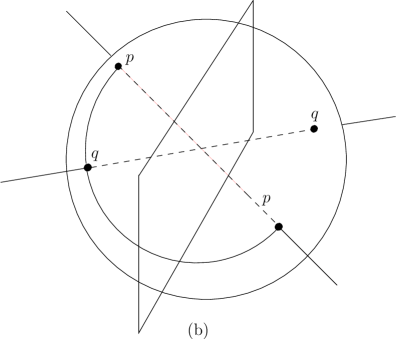
Figure 7: (a) “Walking” in a projective triangulation. (b) Two copies of the edge $pq$, only one is cut by the distinguishing plane.

4 Conclusion and Open Problems

It woud be interesting to check whether the metric on $\mathbb{P}^{2}$ allows to define a triangulation of the projective plane that would extend the notion of Delaunay triangulation, which is well-known in the Euclidean setting. Then, extending the randomized incremental insertion with a hierarchical data-structure such as [2] to the projective case, if possible, would lead to an incremental algorithm with better theoretical (and practical, too) complexity.

Also, problems like the Minimum Weight Triangulation [13], Minmax Length Triangulation [6], etc., may have meaning even on the real projective plane. The Minimum Weight Triangulation problem was neither known to be NP-Hard nor solvable in polynomial time for a long time [8]. This open problem was recently solved and was shown to be NP-Hard by Mulzer and Rote [13]. The Minmax Length Triangulation problem asks about minimizing the maximum edge length in a triangulation of a point set $\mathcal{P}$. This problem was shown to be solvable in time $\mathcal{O}(n^{2})$ by Edelsbrunner and Tan [6]. It would be interesting to analyze the complexity of these problems on the real projective plane $\mathbb{P}^{2}$.

Acknowledgements

The authors would like to thank Olivier Devillers for his valuable suggestions and helpful discussions.

References

- [1] D. W. Barnette. Generating triangulations of the projective plane. J. Combin. Theory Ser. B, 33:222–230, 1982.
- [2] Olivier Devillers. The Delaunay hierarchy. Internat. J. Found. Comput. Sci., 13:163–180, 2002.
- [3] Olivier Devillers and Asish Mukhopadhyay. Finding an ordinary conic and an ordinary hyperplane. Nordic J. Comput., 6:422–428, 1999.
- [4] Olivier Devillers, Sylvain Pion, and Monique Teillaud. Walking in a triangulation. Internat. J. Found. Comput. Sci., 13:181–199, 2002.
- [5] A. K. Dewdney. Wagner’s theorem for the torus graphs. Discrete Math., 4:139–149, 1973.
- [6] H. Edelsbrunner and T. S. Tan. A quadratic time algorithm for the minmax length triangulation. SIAM J. Comput., 22:527–551, 1993.
- [7] David Eppstein. Happy endings for flip graphs. In Proc. 23rd Annual Symposium on Computational Geometry, pages 92–101, 2007.
- [8] M. R. Garey and D. S. Johnson. Computers and Intractability: A Guide to the Theory of NP-Completeness. W. H. Freeman, New York, NY, 1979.
- [9] M. Henle. A Combinatorial Introduction to Topology. W. H. Freeman, San Francisco, CA, 1979.
- [10] L. Kelly and W. Moser. On the number of ordinary lines determined by points. Canad. J. Math., 10:210–219, 1958.
- [11] R. Mori and A. Nakamoto. Diagonal flips in hamiltonian triangulations on the projective plane. Discrete Math., 303:142–153, 2005.
- [12] A. Mukhopadhyay, A. Agrawal, and R. M. Hosabettu. On the ordinary line problem in computational geometry. Nordic J. Comput., 4:330–341, 1997.
- [13] W. Mulzer and Günter Rote. Minimum weight triangulation is NP-hard. Technical Report B-05-23-revised, Freie Universität Berlin, july 2007. http://arxiv.org/abs/cs/0601002.
- [14] S. Negami. Diagonal flips in triangulations on surfaces. Discrete Math., 135:225–232, 1994.
- [15] S. Negami. Diagonal flips in triangulations on closed surfaces, a survey. Yokohama Math. J., 47:1–40, 1999.
- [16] S. Negami and S. Watanabe. Diagonal transformations of triangulations on surfaces. Tsubuka J. Math, 14:155–166, 1990.
- [17] J. Stolfi. Oriented Projective Geometry: A Framework for Geometric Computations. Academic Press, New York, NY, 1991.
- [18] K. Wagner. Bemerkungen zum Vierfarbenproblem. Jahresbericht der Deutschen Mathematiker-Vereinigung, 46:26–32, 1936.
- [19] Afra J. Zomorodian. Topology for Computing. Cambridge University Press, 2005.