A reduced-order strategy for 4D-Var data assimilation

Abstract

This paper presents a reduced-order approach for four-dimensional variational data assimilation, based on a prior EOF analysis of a model trajectory. This method implies two main advantages: a natural model-based definition of a multivariate background error covariance matrix $\textbf{B}_{r}$, and an important decrease of the computational burden of the method, due to the drastic reduction of the dimension of the control space. An illustration of the feasibility and the effectiveness of this method is given in the academic framework of twin experiments for a model of the equatorial Pacific ocean. It is shown that the multivariate aspect of $\textbf{B}_{r}$ brings additional information which substantially improves the identification procedure. Moreover the computational cost can be decreased by one order of magnitude with regard to the full-space 4D-Var method.

, , , , ,

1 Introduction

The aim of this paper is to investigate a reduced-order approach for four-dimensional variational data assimilation (4D-Var), with an illustration in the context of ocean modelling, which is our main field of interest. 4D-Var is now in use in numerical weather prediction centers (e.g. Rabier et al. 2000) and should be a potential candidate for operational oceanography in prospect of seasonal climate prediction and possibly of high resolution global ocean mesoscale prediction. However, ocean scales make the problem even more difficult and computationally heavy to handle than for the atmosphere. Several applications were conducted these last years for various oceanic studies, including for example : basin-scale ocean circulation, either with quasigeostrophic (Moore 1991; Schröter et al. 1993; Luong et al. 1998) or with primitive equation models (Greiner et al. 1998; Wenzel and Schröter 1999; Greiner and Arnault 2000; Weaver et al. 2002); coastal modelling (Leredde et al. 1998; Devenon et al. 2001); or biogeochemical modelling (Lawson et al. 1995; Spitz et al. 1998; Lellouche et al. 2000, Faugeras et al., 2003).

However, although considerable work and improvements have been performed, a number of difficulties remain, common to most applications (and also to other data assimilation methods). The first problem is the fact that ocean models are non-linear, while 4D-Var theory is established in a linear context. More precisely, variational approach can adapt in principle to non-linear models, but the cost function is no longer quadratic with regard to the initial condition (which is the usual control parameter) which can lead to important difficulties in the minimization process and the occurence of multiple minima. Several strategies have been proposed to overcome these problems: Luong et al. (1998) and Blum et al. (1998) perform successive minimizations over increasing time periods; Courtier et al. (1994), with the so-called incremental approach, generate a succession of quadratic problems, which solutions should converge (but with no general theoretical proof) towards the solution of the initial minimization problem. A second major difficulty with variational problem implementation lies in our poor knowledge of the background error, whose covariance matrix plays an important role in the cost function and in the minimization process. In the absence of statistical information, these covariances are often approximated empirically by analytical (e.g. Gaussian) functions. For instance, the covariances, used in the “standard” 4D-Var experiment $E_{FULL}$ described in section 3 are 3D but univariate. Moreover, as discussed in (Lermusiaux, 1999), errors evolve with the dynamics of the system and thus the error space should evolve in the same way. In realistic systems, it proves to be difficult to catch correctly this evolution. The third major problem in the use of 4D-Var in realistic oceanic applications is probably the dimension of the control space. In fact, this dimension is generally equal to the size of the model state variable (composed, in our case, by the two horizontal components of the velocity, temperature and salinity), which is typically of the order of $10^{6}$-$10^{8}$. This makes of course the minimization difficult and expensive (typically tens to hundreds times the cost of an integration of the model), even with the best current preconditioners.

This last difficulty can be addressed by reducing the dimension of the minimization space. This is for example the idea of the incremental approach (Courtier et al. 1994), in which an important part of the successive quadratic minimization problems previously mentioned can be solved using a coarse resolution (e.g. Veersé and Thépaut 1998). The dimension of the minimization problem can then be decreased by one or two orders of magnitude. However, even with such an approach, the dimension of the control space remains quite large in realistic applications. Another way to reduce the dimension of the control space is the representer method (Bennett, 92), performing the minimization in the observation space. The number of parameters to estimate is equal to the number of observation locations. Concerning sequential data assimilation, reduced-order methods were developed to allow the specification of error covariances matrix even for realistic applications. This is the case for example of the Singular Extended Evolutive Kalman (SEEK) filter (Pham et al. 1998; Brasseur et al. 1999).

In this paper, we propose an alternative way for drastically decreasing the dimension of the control space, and hence the cost of the minimization process. Moreover this method provides a natural choice for a multivariate background error covariance matrix, which helps improving the quality of the final solution. The method is based on a decomposition of the control variable on a well-chosen family of a few relevant vectors, and has already been successfully applied in the simple case of a quasigeostrophic box model (Blayo et al. 1998). The aim of the present paper is to further develop this approach and to validate it in a more realistic case, namely a primitive equation model of the equatorial Pacific ocean. The method is described in section 2. Then the model, the assimilation scheme and the numerical experiments are presented in section 3, and their results are discussed. Finally some conclusions are drawn in section 4.

2 The reduced-space approach

Let a model simply written as

$$\frac{\partial{\bf x}}{\partial t}=M({\bf x})$$ (1)

with the state vector ${\bf x}$ in $\Omega\times[t_{0},t_{N}]$, $\Omega$ being the physical domain. Suppose that we have some observations ${\bf y}^{\hbox{\scriptsize o}}$ distributed over $\Omega\times[t_{0},t_{N}]$, with an observation operator $H$ mapping ${\bf x}$ onto ${\bf y}$. The classical 4D-Var approach consists in minimizing a cost function

$$\begin{array}[]{ll}J({\bf u})&=J_{o}({\bf u})+J_{b}({\bf u})\\ &=\frac{1}{2}\,\displaystyle\sum_{i=0}^{N}\left(H({\bf x}_{i})-{\bf y}_{i}^{\hbox{\scriptsize o}}\right)^{T}{\bf R}_{i}^{-1}\left(H({\bf x}_{i})-{\bf y}_{i}^{\hbox{\scriptsize o}}\right)+\frac{1}{2}\,({\bf u}-{\bf u}^{b})^{T}{\bf B}_{u}^{-1}({\bf u}-{\bf u}^{b})\end{array}$$ (2)

using the notations of Ide et al. (1997). ${\bf u}^{b}$ is a background value for the control vector ${\bf u}$, and ${\bf B}_{u}$ is its associated error covariance matrix. In most applications, the control variable ${\bf u}$ is the state variable at the initial time : ${\bf u}={\bf x}(t_{0})$, and the background state ${\bf u}^{b}={\bf x}^{b}$ is typically a forecast from a previous analysis given by the data assimilation system. In this case, once the model is discretized, the size of ${\bf u}$ (i.e. the dimension of the control space ${\cal U}$) is equal to the size of ${\bf x}$, denoted by $n$. $\ \textbf{x}_{i}$ stands for the state variable at time $t_{i}$. In equation (2), $\textbf{x}_{i}$ is propagated by $M$, the fully non-linear model.

In the incremental formulation which is used here, the cost function ${\bf{J}}$ is written as a function of $\delta{\bf x}_{0}={\bf x}_{0}-{\bf x}^{b}$ and the $J_{o}$ term is calculated using the linearized model M:

$$\begin{array}[]{ll}J(\delta\textbf{x})&=\frac{1}{2}(\delta\textbf{x})^{t}\textbf{B}^{-1}\delta\textbf{x}\\ &+\frac{1}{2}\displaystyle\sum_{i=1}^{N}({\bf{H_{i}M_{t_{i},t_{0}}}}\delta\textbf{x}_{0}-\bf{d}_{i})^{t}R_{i}^{-1}({\bf{H_{i}M_{t_{i},t_{0}}}}\delta\textbf{x}_{0}-\bf{d}_{i})\\ \end{array}$$ (3)

where $\bf{d}_{i}$ stands for the innovation vector: $\textbf{d}_{i}=\textbf{y}_{i}-H(\textbf{x}_{b}(t_{i}))$ and $M_{t_{i},t_{0}}$ is the temporal evolution performed by the model $M$ between the instants $t_{0}$ and $t_{i}$.

The basic idea then, for constructing a reduced-order approach, consists in defining a convenient mapping ${\cal M}$ from ${\cal W}\equiv\hbox{\bf IR}^{r}$ into $\,{\cal U}\equiv\hbox{\bf IR}^{n}$, with $r\ll n$, and in replacing the control variable ${\bf u}$ by the new control variable ${\bf w}$ with ${\bf u}={\cal M}({\bf w})$. Since we want to preserve a good solution while having only a rather small number $r$ of degrees of freedom on the choice of ${\bf w}$, the subspace ${\cal M}({\cal W})$ of ${\cal U}$ must be chosen in order to contain only the “most pertinent” admissible values for ${\bf u}$. More precisely, in the case of the control of the initial condition ${\bf u}={\bf x}(t_{0})$, we decide to define the mapping ${\cal M}$ by an affine relationship of the form :

$${\bf x}(t_{0})={\cal M}({\bf w})=\hat{{\bf x}}+\sum_{i=1}^{r}w_{i}{\bf L}_{i}\qquad\hbox{with }{\bf w}=(w_{1},\ldots,w_{r})\in{\cal W}\equiv\hbox{\bf IR}^{r}$$ (4)

In order to let ${\bf w}$ span a wide range of physically possible states, $\hat{{\bf x}}$ represents an estimate of the state of the system, and ${\bf L}_{1},\ldots,{\bf L}_{r}$ are vectors containing the main directions of variability of the system (the $w_{i}$ are scalars). Such a definition relies on the fact that most of the variability of an oceanic system can be described by a low dimensional space. Even if it is only rigorously proved for very simplified models (Lions et al., 1992), it is often expected that, away from the equator, ocean circulation can be seen as a dynamical system having a strange attractor. This means that the system trajectories are attracted towards a (low dimension) manifold. In the vicinity of this attractor, orthogonal perturbations will be naturally damped, while tangent perturbations will not (they can even be greatly amplified, due to the chaotic character of the system). To retrieve a system trajectory over of period of time $[t_{0},t_{N}]$, it seems thus necessary to propose an initial condition ${\bf x}(t_{0})$ containing such variability modes tangent to the attractor, but not necessarily variability modes orthogonal to it. Thus, in definition (4), $\hat{{\bf x}}$ should ideally be located on the attractor, and ${\bf L}_{1},\ldots,{\bf L}_{r}$ should correspond to the main directions of variability tangent to it. In the tropical ocean, the rationale is different, and even simpler since the tropical ocean dynamics is mostly linear, and can be represented by a rather limited number of linear, and possibly non-linear, modes (e.g. De Witte et al. 1998).

In practice, we will choose $\hat{{\bf x}}={\bf x}^{b}$, i.e. the background state that would be used in the corresponding classical 4D-Var approach. With this choice, the increment $\delta{\bf x}={\bf x}(t_{0})-{\bf x}^{b}$ is equal to $\displaystyle{\delta{\bf x}=\sum_{i=1}^{r}w_{i}{\bf L}_{i}={\bf Lw}}$. In this reduced-space approach, we define a new expression for the background term $J_{b}$ of the cost function $J$ :

$$J_{b}({\bf w})=\frac{1}{2}\,{\bf w}^{T}{\bf B}_{w}^{-1}{\bf w}$$ (5)

where ${\bf B}_{w}$ is the background error covariance matrix in the reduced space. The natural representation of ${\bf B}_{w}$ in the full space is the singular matrix

$${\bf B}_{r}={\bf L}{\bf B}_{w}{\bf L}^{T}$$ (6)

Minimization is performed using a quasi-Newton descent method with an exact line search (algorithm M1QN3, Gilbert and Lemaréchal 1989). As in the classical 4D-Var method, the problem is preconditionned by defining a new control variable $\delta{\bf v}=\textbf{B}^{-1/2}\delta{\bf x}_{0}$, which implies $J_{b}(\delta{\bf v})=\frac{1}{2}\,\delta{\bf v}^{T}\delta{\bf v}$. From a programming point of view, this approach implies nearly no modification to the original code, since we only have to add a mapping procedure corresponding to ${\cal M}$, and the adjoint of this procedure.

It is important to point out that the choice of the subspace ${\cal M}({\cal W})$ of ${\cal U}$ is performed using additional information (the information leading to the construction of the ${\bf L}_{i}$s) with regard to usual 4D-Var with no order reduction. This is done of course in order to make the choice of ${\cal M}$ effective, but it will also automatically introduce this extra information into the assimilation procedure (through ${\bf L}$ and ${\bf B}_{w}$), and thus possibly help making the assimilation efficient.

Concerning the actual choice of $({\bf L}_{1},\ldots,{\bf L}_{r})$, different families of vectors can be proposed :

• The variability of the system can be defined in a statistical sense, which means that we seek directions maximizing the variance around a mean state of the system. This is actually the definition of Empirical Orthogonal Functions (EOFs), which can be computed from a sampling of a model trajectory (see section 3.1).

• We can also define the variability in a harmonical sense. In that case, the vectors can be defined by a Fourier or wavelets analysis of a model trajectory. Note however that, with regard to a rectangular domain, the presence of continental boundaries makes the analysis more difficult.

• If we consider the notion of variability within the framework of dynamical systems, we look for vectors maximizing a ratio of the form $\|{\bf x}(t=T_{2})\|/\|{\bf x}(t=T_{1})\|$, for some norm $\|.\|$. The problem can be simplified by making a tangent linear approximation, which leads to the computation of singular vectors (SVs). In the limit case where $T_{2}-T_{1}$ becomes large (infinite), SVs converge towards Lyapunov vectors (LVs). Properties of SVs and LVs can be found for instance in Legras and Vautard (1995). The tangent linear assumption can also be relaxed, and vectors corresponding to SVs and LVs can be computed with the fully non-linear model. They are called respectively non-linear singular vectors (NSVs, Mu 2000) and bred modes (BVs, Toth and Kalnay 1997). Note that, to our knowledge, these “non-linear” vectors have been introduced in an empirical way, with nearly no related properties established theoretically.

Durbiano (2001) performed a thorough study of these families of vectors (EOFs, SVs, LVs, NSVs and BVs) in the perspective of their use as reduced basis for several data assimilation problem. In particular, she compared their performances for the present problem of the control of the initial condition in a reduced space, in the case of a 2-D shallow water model. She concluded in this case to the clear superiority of EOFs with regard to the other families of vectors. This is probably due to the fact that EOFs take into account the nonlinearity of the model (while SVs and LVs do not), and also that their covariance matrix ${\bf B}_{w}$ is quite accurately known, which is not the case for the other families of vectors. That is why we used EOFs in the realistic 3-D experiment described in section 3. Note that this way of approximating the variability of the system in a data assimilation process by a low dimension space generated by the first $r$ EOFs is similar to the method used in the SEEK filter, or in the reduced order filter proposed by Cane et al. (1996).

3 Numerical experiments

3.1 Model and EOF analysis

The model used in our tests is the primitive equation ocean general circulation model OPA (Madec et al. 1999), in its $z$-coordinate rigid-lid version. The region of interest is the equatorial Pacific ocean, from 30^∘S to 30^∘N. The horizontal resolution is set to 1^∘ zonally, and varies meridionally from 1/2^∘ at the equator to 2^∘ at 30^∘. Vertically the ocean is discretized using 25 levels. The state vector consists of temperature, salinity and horizontal velocity, and has a size slightly greater than $10^{6}$.

A one-year simulation was performed, starting from a previous restart built with the ECMWF wind stresses and heat fluxes and using ERS-TAO daily wind stresses and ECMWF heat fluxes to force the model. In a 10^∘-wide band near the northern and southern boundaries, buffer zones are prescribed where the model solution is relaxed towards Levitus climatology. This version of the model has been used previously in a number of studies, and details can be found therein (e.g. Vialard et al. 2001, Vialard et al. 2003, Weaver et al. 2003).

The model solution during the first year of data assimilation experiment (1993) has been sampled with a 2-day periodicity, and a multivariate EOF analysis of the three-dimensional fields has been performed. Let us recall that this analysis consists in determining the main directions of variability of the model sample ${\bf X}=({\bf X}_{1},\ldots,{\bf X}_{p})$, which leads to diagonalizing the covariance matrix ${\bf X}^{T}{\bf X}$, with ${\bf X}_{j}=\displaystyle\frac{1}{\sigma_{i}}[{\bf x}(t_{j})-\bar{\bf x}]$ and $\bar{\bf x}=\displaystyle\frac{1}{p}\,\displaystyle\sum_{j=1}^{p}{\bf x}(t_{j})$. The inner product is the usual one for a state vector containing several physical quantities expressed in different units :

$$<{\bf X}_{j},{\bf X}_{k}>=\sum_{i=1}^{n}\displaystyle\frac{1}{\sigma_{i}^{2}}({\bf x}(t_{j})-\bar{\bf x})_{i}({\bf x}(t_{k})-\bar{\bf x})_{i}$$ (7)

where ${\sigma_{i}^{2}}$ is the empirical variance of the $i$-th component : ${\sigma_{i}^{2}}=\displaystyle\frac{1}{p}\,\displaystyle\sum_{j=1}^{p}({\bf X}_{j}^{i})^{2}$. This diagonalization leads to a set of orthonormal eigenvectors $({\bf L}_{1},\ldots,{\bf L}_{p})$ corresponding to eigenvalues $\lambda_{1}>\ldots>\lambda_{p}>0$. Since trajectories are computed with the fully non-linear model, these modes represent non-linear variability around the mean state over the whole period.

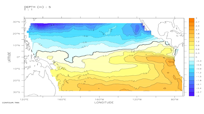
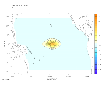
The first level ($z=5$m) of the first EOF is displayed on Fig. 1. As can be seen, it is mostly representative of the variability of the equatorial zonal currents, of the north-south temperature oscillation and of the mean structure of the sea surface salinity.

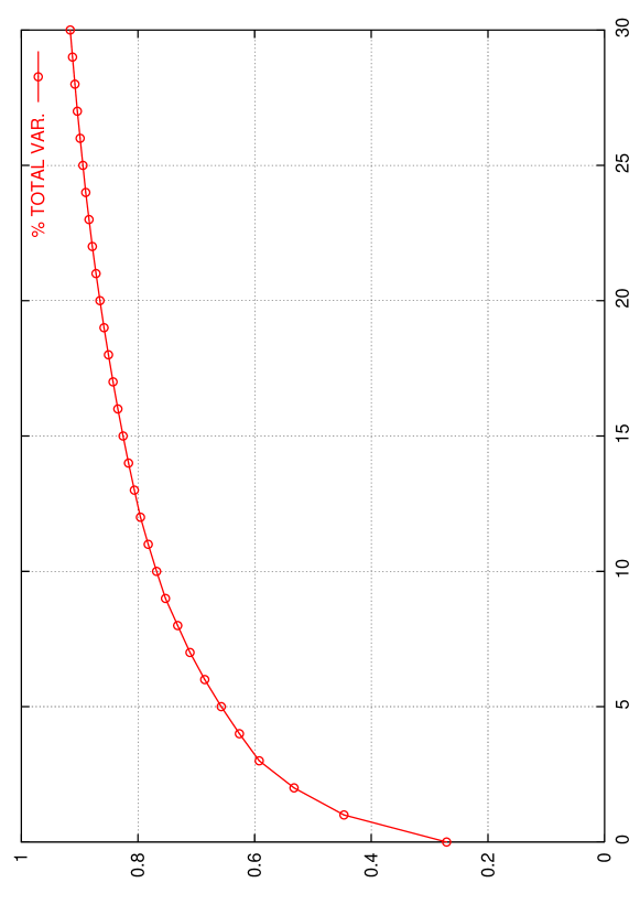
The fraction of variability (or “inertia”) which is conserved when retaining only the $r$ first vectors is $\displaystyle\sum_{j=1}^{r}\lambda_{j}/\sum_{j=1}^{p}\lambda_{j}$. Its variation as a function of $r$ is displayed in Fig. 2. We can see that a large part of the total variance can be represented by a very few EOFs : 80% for the first 13 EOFs, 92% for the first 30 EOFs.

Finally, let us emphasize that a natural estimate for the covariance matrix of the first $r$ eigenvectors $({\bf L}_{1},\ldots,{\bf L}_{r})$, i.e. ${\bf B}_{w}$ in our reduced-order 4D-Var, is simply the diagonal matrix $\hbox{Diag}(\lambda_{1},\ldots,\lambda_{r})$.

3.2 Assimilation experiments

A 4D-Var assimilation scheme, based on the incremental formulation of Courtier et al. (1994), has been developped for the OPA model (Weaver et al. 2003, Vialard et al. 2003). Without going into details (which can be found in references above), let us recall that the nonquadratic cost function $J({\bf x}(t_{0}))$ is expressed in terms of the increment $\delta{\bf x}_{0}$, and that its minimization is replaced by a sequence of minimizations of simplified quadratic cost functions. The basic state-trajectory used in the tangent linear model is regularly updated in an outer loop of the assimilation algorithm, while the iterations of the actual minimizations are performed within an inner loop.

Different statistical models can be chosen for representing the correlations of background error. In the present study, we used a Laplacian-based correlation model, which is implemented by numerical integration of a generalized diffusion-type equation (Weaver and Courtier, 2001). The horizontal correlation lengths for the gaussian functions are equal to $8^{o}$ in longitude and $2^{o}$ in latitude near the equator and $4^{o}$ in longitude/latitude outside the area situated between $20^{o}$N/S. The vertical correlation lengths depend on the depth. ${\bf B}$ is thus block diagonal : covariances are spatially varying but remain monovariate. Such a choice for ${\bf B}$ leads to significantly better results than those given by a simple diagonal representation of this matrix. However, since ${\bf B}$ remains univariate, the links between the model variables come only from the action of the model dynamics. The development of a multivariate model for ${\bf B}$ is presently under way in research groups. Ricci et al. (2004) include a state-dependent temperature-salinity constraint, which works quite well in the 3D-Var case but is not yet operational for the 4D-Var case.

The observation error covariance matrices ${\bf R}_{i}$ depend of course of the assimilated data. We will consider in the present case only temperature observations, which are assumed independent with a standard error equal to $\sigma_{T}$. The ${\bf R}_{i}$ are thus taken equal to $\sigma_{T}^{2}\,{\bf Id}$.

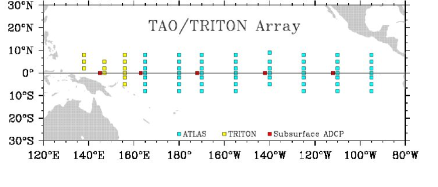
We have used for our experiments the classical framework of twin experiments. A one-year simulation of the model was performed, starting at the beginning of 1993. This simulation (further denoted $E_{REF}$) will be the reference experiment. Pseudo-observations of the temperature field were then generated, by extraction from this one-year solution at the locations of the 70 TAO moorings (Fig. 3), with a periodicity of 6 hours, on the first 19 levels of the model (i.e. the first 500 meters of the ocean). This corresponds to observing 0.17% of the model state vector every 6 hours. Those temperature values have been perturbed by the addition of a gaussian noise, with a standard error set to $\sigma_{T}=0.5$^∘C, which is an upper bound for the standard error of the real TAO temperature dataset.

A 4D-Var assimilation of these pseudo-observations (i.e. with full control variable $\delta{\bf x}_{0}$, built from the state vector (u,v,T,S) in the whole space) was then performed, using an independent field ${\bf x}_{b}$ (a solution of the model three months later) as the first guess (background field) for the minimization process. This first assimilation experiment will be denoted $E_{FULL}$, since it uses the full control space. In order to improve the validity of the tangent linear approximation, the assimilation time window was divided into successive one-month windows.

Then an additional simulation was performed, using the reduced-space approach described in section 2 with $r=30$ EOFs (which represent 92% of the total inertia - Fig. 2). This second assimilation experiment will be denoted $E_{REDUC}$. As detailed previously, the control variable in this case is ${\bf w}=(w_{1},\ldots,w_{r})$, with the mapping $\delta{\bf x}_{0}={\bf L}{\bf w}$ and the preconditionning $\delta{\bf v}={\bf B}_{w}^{-1/2}{\bf w}={\bf B}_{w}^{-1/2}{\bf L}^{T}\delta{\bf x}_{0}$.

3.3 Numerical results

As explained in section 2, the reduced-space assimilation algorithm presents two main differences with regard to the full-space algorithm, which are the multivariate nature of the background error covariance matrix, and the small dimension of the control space. Both aspects are expected to improve the efficiency of the assimilation, and we will now illustrate their respective impact.

3.3.1 Background error covariances

The background error covariance matrix used in the reduced-space approach is defined empirically by the EOF analysis and is expressed in the full-space as ${\bf B}_{r}={\bf L}{\bf B}_{w}{\bf L}^{T}$. It integrates statistical information on the consistency between the different model variables, and is naturally multivariate. On the other hand, the matrix ${\bf B}$ used in the full-space 4D-Var is univariate, since providing a multivariate model for this matrix remains challenging. This aspect is of course very important, and should lead to significant changes in the assimilation results. Note that Buehner et al. (1999) have proposed a similar way of representing error covariances with EOF analysis in the context of 3D-Var. However they consider that the reduced basis is not sufficient to span the analysis increment space and blend this EOF basis with the prior ${\bf B}$ projected into the sub-space orthogonal to the EOFs.

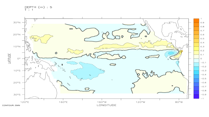
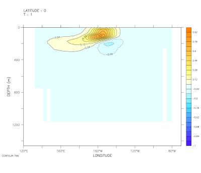
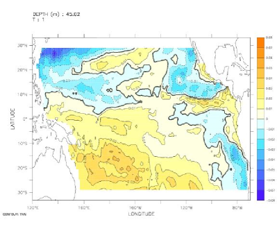
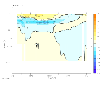
An interesting way to illustrate these differences between the full-space ${\bf B}$ and the reduced-space ${\bf B}_{r}$ is to perform preliminary assimilation experiments with a single observation. For that purpose, we use a single temperature observation located within the thermocline at 160^∘W on the equator, and specified at the end of a one-month assimilation time window. The innovation is set to 1^∘K. The analysis increment at the initial time in such an experiment is proportional to the column of ${\bf B}{\bf M}_{t_{n},t_{0}}^{T}$ corresponding to the location of the observation. As can be seen in Fig. 4, the reduced-space method performs, as expected, a rather weak correction over the whole basin, while the full-space method generates a much stronger and local increment. The structure of the increment is indeed much more elaborate in the reduced-space experiment, with scales larger than in the full-space experiment. Note that the input from the first EOF (shown on Fig. 1) is quite clear in the horizontal pattern of the increment, since $w_{1}/\|{\bf w}\|=0.86$ in this particular case. The maximum value of the increment however is only 0.06^∘C for the reduced-space 4D-Var, while it is 0.94 ^∘C in the full-space 4D-Var.

The interest of the naturally multivariate aspect of ${\bf B}_{r}$ is also clear in the results of our twin experiments. Two different types of diagnostics were performed, the first one concerning only the assimilated variables (i.e. temperature in the present case), while the second one relates to all other variables that are not assimilated. This second type of diagnostic is of course the most significant, since it evaluates the capability of the assimilation procedure to propagate information over the whole model state vector.

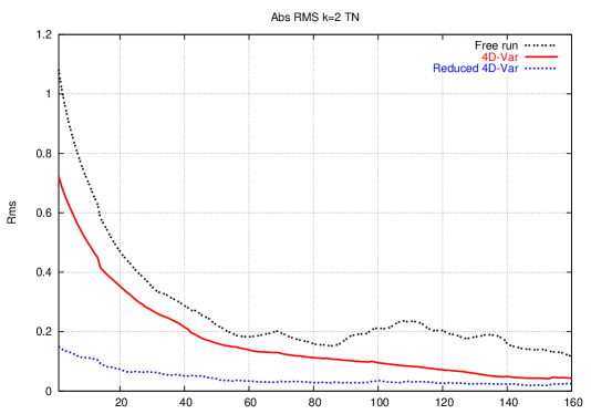
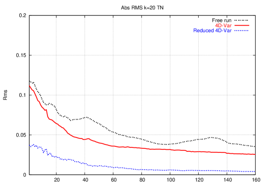
An example of the first type of diagnostic is given in Fig. 5a, which displays the temperature rms error defined by

$$\hbox{rms}_{T}(z,t)=\left(\int{\left(T(\lambda,\theta,z,t)-T_{REF}(\lambda,\theta,z,t)\right)^{2}d\lambda\,d\theta}\right)^{1/2}$$ (8)

The discretized formula becomes :

$$\hbox{rms}_{T}(z,t)=\|x-x_{ref}\|_{2}=\left[\displaystyle\frac{1}{N_{x}\times N_{y}}\sum_{i=1}^{N_{x}}\sum_{j=1}^{N_{y}}(\textbf{T}(i,j,z,t)-\textbf{T}_{ref}(i,j,z,t))^{2}\right]^{1/2}$$ (9)

where $N_{x}$ and $N_{y}$ are the number of grid points in x and y. This error is significantly weaker in $E_{REDUC}$ than in $E_{FULL}$, although the assimilation system in $E_{REDUC}$ has much less degrees of freedom to adjust the model trajectory to these data.

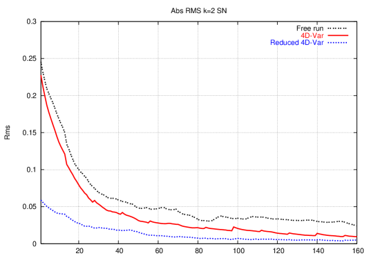
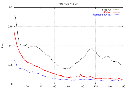
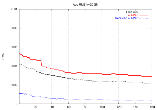
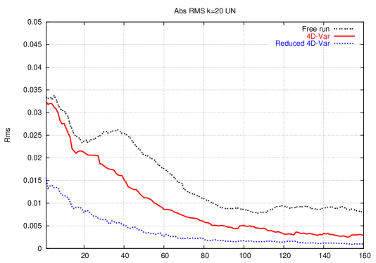
An example of the second type of diagnostic is shown in Fig. 5b,c. In our test case, these results are clearly in favour of the reduced-space approach. The errors on the salinity S and the zonal component of the velocity $u$ for the solution provided by $E_{FULL}$ are systematically greater than for $E_{REDUC}$.

The interest of this approach can also be illustrated by the results in the lower levels. It is well-known that the time-scale for the information to penetrate from the upper ocean into the deep ocean within an assimilation process may be quite long. However, in experiment $E_{REDUC}$ the EOFs add information on the vertical structure of the flow (see Fig. 4) and then make the vertical adjustment easier. We have plotted for example in Fig. 6 the errors of the different solutions at level 20 (depth : 750 m, ie below the observations). $E_{REDUC}$ performs a very good identification of the solution due to the propagation of the information in depth.

These results are only part of what should be shown in terms of diagnostic analyses. But all of them clearly prove that the results of $E_{REDUC}$ vs $E_{FULL}$ are significantly improved for all, assimilated or not, variables.

Finally, it must be mentioned that we have also illustrated the fundamental role of the multivariate nature of ${\bf B}_{r}$ by performing an additional reduced-order experiment (not shown) using univariate EOFs. In this case, the directions proposed for the minimization were not relevant, and the assimilation failed.

3.3.2 Dimension of the control space

The second important difference brought by the reduced-space approach with regard to the full-space approach is the dimension of the minimization space, which is decreased by several orders of magnitude. This should reduce the number of iterations necessary for the minimization, i.e. reduce the cost of the data assimilation algorithm, which is an important practical issue.

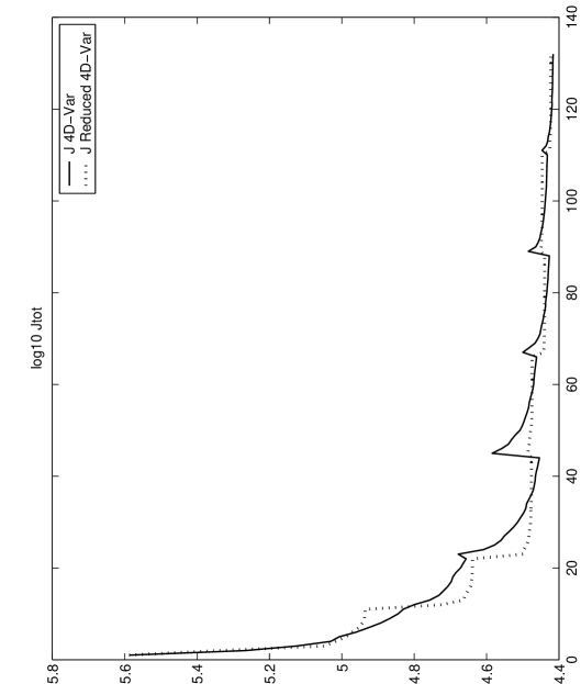
The evolution of the cost functions for experiments $E_{FULL}$ and $E_{REDUC}$ are displayed on Fig. 7. Since we use different covariance matrices ${\bf B}$ and ${\bf B}_{r}$ in these two experiments, the curves are not quantitatively comparable. However, it is clear in Fig. 7 that the number of iterations required to stabilize the cost function is reduced by nearly one order of magnitude between the full-space 4D-Var approach (which needs typically several tens of iterations) and the reduced-space approach (which needs eight to ten iterations). In the present experiments, we have kept the same number of iterations (2 outer loops of ten iterations each) in the two experiments to strictly compare the results. But having a look at the cost function, it is clear that the minimum is quickly reached by $E_{REDUC}$ experiment. Considering the low number of freedom degrees, the computational cost can be thus divided by a factor of 4 or 5 between the two methods.

4 Conclusion

This paper presents a reduced-space approach for 4D-Var data assimilation. A new control space of low dimension is defined, in which the minimization is performed. An illustration of the method is given in the case of twin experiments with a primitive equation model of the equatorial Pacific ocean.

This method presents two important features, which make the assimilation algorithm effective. First the background error covariance matrix ${\bf B}_{r}$ is built using statistical information (an EOF analysis) on a previous model run. This introduces relevant additional information in the assimilation process and makes ${\bf B}_{r}$ naturally multivariate, while providing an analytical multivariate model for ${\bf B}$ is still challenging. This improves the identification of the solution, both on observed and non-observed variables, and at all depths in the model. Secondly the reduction of the dimension of the control space limits the number of iterations for the minimization, which results in a decrease of the computational cost by roughly one order of magnitude.

However the results presented in this work are only a first (but necessary) step, since they concern twin experiments. They need of course to be confirmed by additional experiments in other contexts, in particular experiments with real data and in other geographical areas. As a matter of fact, the efficiency of the method is closely related to the fact that the reduced basis does contain pertinent information on the variability of the true system. That is why, in the context of real observations (i.e. in the case of an imperfect model), the control space must probably not be limited to model-based variability. Therefore, we can imagine either compute EOFs from results of previous data assimilation using for example full-space 4D-Var (Durbiano 2001), and/or improve the assimilation results by performing a few full-space iterations at the end of the reduced-space minimization (Hoteit et al. 2003).

Several other ideas can be considered to extend the present methodology to a fully realistic context, and some of them are presently under investigation in our group. Concerning the definition of the reduced basis, one could think of its evolutivity and adaptivity, as in some sequential assimilation methods (Brasseur et al. 1999; Hoang et al. 2001). Moreover a major source of difficulty (common to all data assimilation methods) is our insufficient knowledge (and therefore parameterization) of the model error. Recent works have addressed this problem in the context of variational methods, which intend to model and control this error (e.g. D’Andréa and Vautard 2001; Durbiano 2001; Vidard 2001). Such a control could probably be performed in a reduced-order context and complement efficiently the present method.
Acknowledgments

The authors would like to thank Anthony Weaver and Arthur Vidard for numerous helpful discussions. A. Weaver provided the OPAVAR package and helped us using it. Laurent Parent helped in the configuration of the numerical experiments. This work has been supported by the french project MERCATOR for operational oceanography. Idopt is joint CNRS-INPG-INRIA-UJF research project.

Figure 1: First EOF. Top: surface temperature; Middle: surface salinity; Bottom: surface velocity. The quantities are non-dimensional.

Figure 2: Fraction of inertia conserved by the $r$ first EOFs : $\sum_{j=1}^{r}\lambda_{j}/\sum_{j=1}^{p}\lambda_{j}$ as a function of $r$

Figure 3: Locations of the TAO morrings.

Figure 4: Temperature component of the optimal increment $\delta{\bf x}_{0}$ for single observation experiments. Left : horizontal structure at $z=-45$ m; right : vertical section along the equator. Top : full-space 4D-Var; bottom : reduced-space 4D-Var.

a)

b)

c)

Figure 5: Rms error with respect to the exact reference solution at level 2 (depth: 15 m). $x$-axis : time (in days). $y$-axis : (a) $T$ (^∘K), (b) $S$ (kg.m${}^{-3})$, (c) $u$ (m.s^-1). The curves correspond to experiment $E_{REF}$ (dotted line), $E_{FULL}$ (solid line) and $E_{REDUC}$ (dotted line).

a)

b)

c)

Figure 6: Same as Fig. 5, but at level 20 (depth: 750 m).

Figure 7: Cost functions vs iterations. Solid line: experiment $E_{FULL}$ (22 iterations for each of the six one-month assimilation time-windows); Dotted line: experiment $E_{REDUC}$ (22 iterations for each of the six one-month assimilation time-windows)

References

- [1] Bennett, A. F., 1992: Inverse methods in physical oceanography. Cambridge Monographs on Mechanics and Applied Mathematics. Cambridge University Press.
- [2] Blayo, E., Blum, J. and Verron, J., 1998: Assimilation variationnelle de données en océanographie et réduction de la dimension de l’espace de contrôle. Pp. 199–219 in Equations aux Dérivées Partielles et Applications. Gauthier-Villars.
- [3] Blum, J., Luong, B. and Verron, J., 1998: Variational assimilation of altimeter data into a non-linear ocean model: temporal strategies. ESAIM Proceedings, 4, 21–57.
- [4] Brasseur, P., Ballabrera-Poy, J. and Verron, J., 1999: Assimilation of altimetric data in the mid-latitude oceans using the Singular Evolutive Extended Kalman filter with an eddy-resolving primitive equation model. J. Mar. Syst., 22, 269–294.
- [5] Buehner, M., Brunet, G. and Gauthier, P., 1999: Empirical orthogonal functions for modeling 3D-Var forecast error statistics. Pp. 324–327 in Proceedings of the Third WMO International Symposium on Assimilation of Observations in Meteorology and Oceanography, 7–11 June 1999, Quebec City, Canada.
- [6] Gauthier, P., Buehner, M. and Fillion, L., 1998: Background-error statistics modelling in a 3D variational data assimilation scheme: estimation and impact on the analyses. P-p 131–145 in Proceedings of the ECMWF Workshop on the diagnostics of assimilation systems, 2-4 November 1998, Reading, U.K.
- [7] Cane, M. A., Kaplan, A., Miller, R. N., Tang, B., Hackert, E. C. and Busalacchi, A. J., 1996: Mapping tropical Pacific sea level: Data assimilation via a reduced state Kalman filter. J Geophys. Res., 101, 22599–22617.
- [8] Courtier, P., Thépaut, J.-N. and Hollingsworth, A., 1994: A strategy for operational implementation of 4D-Var, using an incremental approach. Q. J. R. Meteorol. Soc., 120, 1367–1388.
- [9] D’Andréa, F. and Vautard, R., 2001: Reducing systematic errors by empirically correcting model errors. Tellus, 52, 21–41.
- [10] Devenon, J.-L., Dekeyser, I., Leredde, Y. and Lellouche, J.-M., 2001: Data assimilation method by a variational methodology using the adjoint of a 3-D coastal circulation primitive equation model. Oceanol. Acta, 24, 395–407.
- [11] De Witte, B., Reverdin, G. and Maes, C., 1998: Vertical structures of an OGCM simulation of the equatorial Pacific ocean in 1985-1994. J. Phys. Oceanogr., 29, 1542–1570.
- [12] Durbiano, S., 2001: Vecteurs caractéristiques de modèles océaniques pour la réduction d’ordre en assimilation de données. PhD thesis, University of Grenoble.
- [13] Faugeras, B., Levy, M., Memery, L., Verron, J., Blum, J. and Charpentier, I., 2003: Can biogeochemical fluxes be recovered from nitrate and chlorophyll data ? A case study assimilating data in the Northwestern Mediteranean Sea at the JGOFS-DYFAMED station. Jour. of Mar. Sys., 40-41, 99–125.
- [14] Gilbert, J.-C. and Lemaréchal, C., 1989: Some numerical experiments with variable storage quasi-Newton algorithms. Mathematical programming, 45, 407–435.
- [15] Greiner, E., Arnault, S. and Morlière, A., 1998: Twelve monthly experiments of 4D-variational assimilation in the tropical Atlantic during 1987. Part 1: method and statistical results. Progr. Oceanogr., 41, 141–202.
- [16] Greiner, E. and Arnault, S., 2000: Comparing the results of a 4D-variational assimilation of satellite and in situ data with WOCE CITHER hydrographic measurements in the tropical Atlantic. Prog. Oceanogr., 47, 1–68.
- [17] Hoang, H.S., Baraille, R. and Talagrand, O., 2001: On the design of a stable adaptive filter for state estimation in high dimensional systems. Automatica, 37, 341–359.
- [18] Hoteit, I., Khol, A., Stammer, D. and Heimbach, P., 2003: A reduced-order optimization strategy for four dimensional variational data assimilation. In Proceedings of EGS-AGU-EUG Joint Assembly, 6-11 April 2003, Nice, France.
- [19] Ide, K., Courtier, P., Ghil, M. and Lorenc, A. C., 1997: Unified notation for data assimilation: operational, sequential and variational. J. Meteorol. Soc. Jpn, 75, 181–189.
- [20] Lawson, L. M., Spitz, Y. H., Hofman, B. E. and Long, R. B., 1995: A data assimilation technique applied to a predator-prey model. Bull. Math. Biol., 57, 593–617.
- [21] Legras, B. and Vautard, R., 1995: A guide to Liapunov vectors. Pp. 143–156 in Proceedings of the ECMWF seminar on Predictability.
- [22] Lellouche, J.-M., Ouberdous, M. and Eifler, W., 2000: 4D-Var data assimilation system for a coupled physical-biological model. Earth and Planetary Science, 109, 491–502.
- [23] Lermusiaux, P. J. F. and Robinson, A. R., 1999: Data Assimilation via Error Subspace Statistical Estimation. Part I: Theory and Schemes. Mon. Wea. Rev., 127, 1385–1407.
- [24] Leredde, Y., Lellouche, J.-M., Devenon, J.-L. and Dekeyser, I., 1998: On initial, boundary conditions, and viscosity coefficient control for Burger’s equation. Int. J. Num. Meth. Fluids, 28, 113–128.
- [25] Lions, J.L., Temam, R. and Wang, S., 1992: On the equation of large scale Ocean. Nonlinearity, 5, 1007–1053.
- [26] Luong, B., Blum, J. and Verron, J., 1998: A variational method for the resolution of a data assimilation problem in oceanography. Inverse Problems, 14, 979–997.
- [27] Madec, G., Delecluse, P., Imbard, M. and Levy, C., 1999: OPA release 8.1, Ocean general circulation maodel reference manual. Internal report, LODYC/IPSL, France.
- [28] Moore, A. M., 1991: Data assimilation in a quasigeostrophic open-ocean model of the Gulf-Stream region using the adjoint model. J. Phys. Oceanogr., 21, 398–427.
- [29] Mu, M., 2000: Nonlinear Singular Vectors and Nonlinear Singular Values. Science in China, 43(D), 375–385.
- [30] Pham, D. T., Verron, J. and Roubaud, M.-C., 1998: A singular evolutive extended Kalman filter for data assimilation in oceanography. J. Mar. Syst., 16, 323–340.
- [31] Rabier, F., Jarvinen, H., Klinker, E., Mantouf, J.-F. and Simmons, A., 2000: The ECMWF operational implementation of 4D-Var assimilation. Part I: experimental results with simplified physics. Q. J. R. Meteorol. Soc., 126, 1143–1170.
- [32] Ricci, S., Weaver, A. T., Vialard, J. and Rogel, P. 2005: Incorporating state-dependent Temperature-Salinity constraints in the background error covariance of variational ocean data assimilation. Mon. Wea. Rev., 133, 317–338.
- [33] Schröter, J., Seiler, U. and Wenzel, M., 1993: Variational assimilation of Geosat data into an eddy-resolving model of the Gulf Stream area. J. Phys. Oceanogr., 23, 925–953.
- [34] Spitz, Y. H., Moisan, J. R., Abbott, M. R. and Richman, J. G., 1998: Data assimilation and a pelagic ecosystem model: parameterization using time series observations. J. Mar. Syst., 16, 51–68.
- [35] Toth, Z. and Kalnay, E., 1997: Ensemble forecasting at NCEP : the breeding method. Mon. Weather Rev., 125, 3297–3318.
- [36] Veersé, F. and Thépaut, J.-N., 1998: Multiple-truncation incremental approach for four-dimensional variational data assimilation. Q. J. R. Meteorol. Soc., 125, 1889–1908.
- [37] Vialard, J., Menkes, C., Boulanger, J.-P., Delecluse, P., Guilyardi, E., McPhaden, M. J. and Madec, G., 2001: A model study of oceanic mechanisms affecting equatorial Pacific sea surface temperature during the 1997-98 El Nino. J. Phys. Oceanogr., 31, 1649–1675.
- [38] Vialard, J., Vialard, A. T., Anderson, D. L. T. and Delecluse, P., 2003: Three- and four-dimensional variational assimilation with a general circulation model of the tropical Pacific ocean. Part II: Physical validation. Mon. Wea. Rev., 131, 1379-1395.
- [39] Vidard, P., 2001: Vers une prise en compte des erreurs modèle en assimilation de données 4D variationnelle. Application à un modèle d’océan. PhD thesis, University of Grenoble.
- [40] Weaver, A. T. and Courtier, P., 2001: Correlation modelling on the sphere using a generalized diffusion equation. Q. J. R. Meteorol. Soc., 127, 1815–1846.
- [41] Weaver, A. T., Vialard, J., Anderson, D. L. T. and Delecluse, P., 2003: Three- and four-dimensional variational assimilation with a general circulation model of the tropical Pacific ocean. Part I: Formulation, internal diagnostics and consistency checks. Mon. Wea. Rev., 131, 1360-1378.
- [42] Wenzel, M. and Schröter, J., 1999: 4D-Var data assimilation into the LSG OGCM using integral constraints’. Pp. 141–144 in Proceedings of the Third WMO International Symposium on Assimilation of Observations in Meteorology and Oceanography, 7-11 June 1999, Quebec City, Canada.