Reduced-order 4D-Var: a preconditioner for the Incremental 4D-Var data assimilation method

C. Robert E. Blayo LMC-IMAG, CNRS-INPG-INRIA-UJF J. Verron LEGI, CNRS-INPG-UJF

Abstract

This study demonstrates how the incremental 4D-Var data assimilation method can be applied efficiently preconditioned in an application to an oceanographic problem. The approach consists in performing a few iterations of the reduced-order 4D-Var prior to the incremental 4D-Var in the full space in order to achieve faster convergence. An application performed in the tropical Pacific Ocean, with assimilation of TAO temperature data, shows the method to be both feasible and efficient. It allows the global cost of the assimilation to be reduced by a factor of 2 without affecting the quality of the solution.

\authorrunninghead

Robert et al. \titlerunningheadPreconditioning 4D-Var data assimilation method \authoraddrC. Robert, LMC-IMAG, BP 53, 38041 Grenoble Cedex 9, France (Celine.Robert@imag.fr) {article}

1 Introduction

Computational requirements remain a major limiting factor for operational forecasting of atmospheric and oceanic circulations. In such systems, most of the computation resources are generally devoted to data assimilation: typically, sequential data assimilation may cost one order of magnitude more than a model simulation, and variational data assimilation two orders of magnitude more. Even allowing for the evolution of computer technology, such constraints seem likely to remain for many years to come since numerous scientific studies have shown that an increase in model resolutions is needed per se. Within this context, the aim of this letter is to report on how a reduced-order approach to variational data assimilation can help decrease the computational cost of this method.

2 Full space and reduced order Incremental 4D-Var

The usual method employed for variational assimilation in current meteorological and oceanographical applications is the incremental 4D-Var [Courtier et al., 1994]. This method aims at determining an optimal correction $\delta\textbf{x}$ , defined in the full space, to a first approximation $\textbf{x}^{b}$ of the initial condition, which minimizes a functional

$\displaystyle J(\delta\textbf{x})$	$\displaystyle=$	$\displaystyle J_{b}(\delta\textbf{x})+J_{o}(\delta\textbf{x})$
	$\displaystyle=$	$\displaystyle\frac{1}{2}(\delta\textbf{x})^{T}\textbf{B}^{-1}\delta\textbf{x}$
	$\displaystyle+\frac{1}{2}$	$\displaystyle\sum_{i=1}^{N}({\bf{H_{i}M_{i}}}\delta\textbf{x}-\bf{d}_{i})^{T}R_{i}^{-1}({\bf{H_{i}M_{i}}}\delta\textbf{x}-\bf{d}_{i})$	(2)

where $\textbf{M}_{i}$ is the tangent linear model between the initial time $t_{0}$ and time $t_{i}$ , and $\textbf{H}_{i}$ is the observation operator, linearized at time $t_{i}$ . The innovation vector, $\textbf{d}_{i}$ , is the difference between the observation vector $\textbf{y}_{i}$ and its model equivalent at time $t_{i}$ : $\bf{d}_{i}=\textbf{y}_{i}-{\bf{H_{i}M_{i}\textbf{x}_{b}}}$ .
The background error covariance matrix B is generally rather poorly known, and its definition presents a difficult problem. This lack of suitable definition impacts strongly on the quality of the solution and has been the subject of numerous research studies. In the usual incremental 4D-Var approach, B may be defined analytically, using, for example, monovariate gaussian-like covariances, and balance equations for multivariate covariances.

In a reduced-order approach (hereafter denoted R-4D-Var), B and $\delta\textbf{x}$ are specified in a low-dimension subspace which contains a large part of the natural variability of the system. An efficient way to build such a subspace is to define it as the span of a few EOFs, $\textbf{L}_{i}$ ( $i=1,\ldots,r$ ), computed from previous model simulations [Blayo et al., 1998; Durbiano, 2001; Robert et al., 2005].

Formally, $J_{o}$ remains unchanged, and only the expressions for $\delta$ x and B change in $J_{b}$ . The increment $\delta$ x is expanded in the EOFs basis $\displaystyle{\delta\textbf{x}=\displaystyle\sum_{i=1}^{r}w_{i}\textbf{L}_{i}=\textbf{Lw}}$ , and B is then naturally represented by the low-rank matrix $\displaystyle{\textbf{B}_{r}=\textbf{L}\boldsymbol{\Lambda}_{r}\textbf{L}^{T}}$ with $\boldsymbol{\Lambda}_{r}=diag(\lambda_{1},...,\lambda_{r})$ where $\lambda_{i}$ is the eigenvalue corresponding to $\textbf{L}_{i}$ (see Robert et al., 2005 for details). Thus, $\textbf{B}_{r}$ naturally contains 3-D multivariate covariances. Note that another stategy consists in reducing the model itself using a POD approach [Cao et al., 2005; Daescu and Navon, 2006].

Both full space and reduced-order 4D-Var methods have been applied in the context of data assimilation in a primitive equation model of the tropical Pacific Ocean. The model is the OPA code [Madec et al., 1998] in its so-called TDH configuration, with the variational data assimilation package OPAVAR [Weaver et al., 2003]. Numerous earlier studies have been conducted using this configuration with the incremental 4D-Var, assimilating TAO and XBT temperature profiles, and have produced good results [Weaver et al., 2003; Vialard et al., 2003]. In these studies, the background error covariance matrix B is defined as an operator including gaussian-like covariance functions, but it remains monovariate [Weaver and Courtier, 2001]. Efforts to develop a multivariate operator have been made recently and implemented in the 3D-Var context [Ricci et al., 2005].

This incremental 4D-Var approach needs quite a large number of iterations -typically 40- to converge [Vialard et al., 2003, Weaver et al., 2003]. Since each iteration requires one run of both the tangent linear model and the adjoint model, the computational cost can thus become prohibitive for real configurations. In a non-linear situation such as the mid-latitude ocean, the cost will be even greater [Blum et al., 1998].

By working only in a low-dimension space, and thereby optimizing a very limited number of coefficients (we have retained 30 EOFs vectors, explaining 92 $\%$ of the total variability), the R-4D-Var tries in particular to overcome this drawback. This method has proved to work well in the idealized context of twin experiments, i.e. when the model assimilates simulated observations and is thus supposed to be perfect [Robert et al., 2005]. The computational cost is decreased in this case by a factor of at least 3, and the optimal increment is very well identified in the space spanned by the EOFs.

3 A Two-Step 4D-Var strategy

When dealing with real data, the definition of a relevant EOF basis, representative of the true variability of the system, is much more challenging. Since the model has significant errors, EOFs computed from model simulations without assimilation do not contain the right information and lead to poor R-4D-Var results. One possible way to address this difficulty is to compute EOFs from a previous assimilated run, with another assimilation method for example. However, since the system providing the EOFs remains in any case imperfect, the low-dimension correction subspace does not contain all the relevant variability of the true dynamics. The key idea of this study is therefore to combine the quality of the identification performed by 4D-Var and the efficiency of R-4D-Var. This means that we continue to look for an optimal correction $\delta\textbf{x}$ in the full space, but address the problem of the associated high computational cost by using R-4D-Var to provide a relevant initial guess for full space minimization. The approach consists thus in performing a few iterations of R-4D-Var (without trying to reach a converged solution), and in using this current estimate of $\delta\textbf{x}$ to initialize additional iterations of 4D-Var. Only a few of the first iterations of R-4D-Var appear to be effective in providing a relevant first guess, defined in the reduced space. This first guess can then be corrected and improved in the full space by a few iterations of 4D-Var. This technique can thus be seen as a preconditioning of 4D-Var by R-4D-Var, and will hereafter be referred to as “Two-Step 4D-Var” (TS-4D-Var). Note that the expression of B changes between R-4D-Var and 4D-Var. This means that the role of $J_{b}$ is identical in both methods (to minimize $\|\delta\textbf{x}\|$ ) but with different norms. The other functional $J_{0}$ remains unchanged. The cost functions being quadratic (due to the incremental approach), any unconstrained minimization algorithm may be used. We use here a BFGS-like algorithm.

4 Assessing the Two-Step strategy

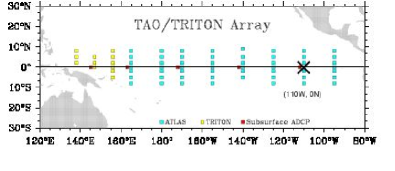
In order to validate this TS strategy, experiments are performed in the tropical Pacific Ocean (Fig. 1), using the OPA model in its TDH configuration. The atmospheric forcings are daily ERS-TAO winds [Menkes et al., 1998] and monthly ECMWF heat fluxes. Our experiments start in January 1993 and last one year. The dynamics during this period is representative of a ”normal” year in the tropical Pacific, without the noteworthy influence of any ENSO event. These conditions are seen as favorable to test the method.

In order to be able to compare our results with those of previous studies performed with the same configuration [Vialard et al., 2003], we assimilate temperature data from the TAO/TRITON array plus XBT.

In the TS-4D-Var, we first perform 10 iterations of the R-4D-Var. These are followed by a run of the fully non-linear direct model in order to update the reference trajectory for linearization. Then, 10 iterations of the incremental 4D-Var are performed. Thus, the cycle of the TS-4D-Var is like a cycle of the 4D-Var with 2 outer loops consisting of 10 inner loops each.

Figure 2 shows the two successive sequences of the observation term $J_{o}$ in the cost function. We can see that the R-4D-Var performs a first descent (10 iterations, although 5-6 may be sufficient) followed by a second one performed by the incremental 4D-Var. The second sequence allows us to reach a lower level very quickly and to stabilize the value of the cost function after very few iterations. Thus, the minimization phase requires a lower number of iterations to reach the minimum (less than 20, whereas 40 are required with the incremental 4D-Var), due to the fact that we retain only the 30 largest EOF vectors.

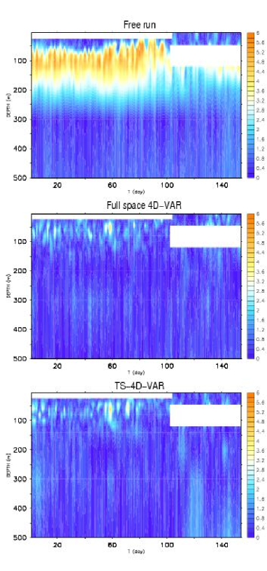
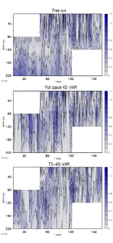
For both assimilated and non-assimilated variables, the TS-4D-Var provides results that are definitely comparable to those obtained with the incremental 4D-Var. To illustrate this point, Figures 3 and 4 show a comparison of the fields at a particular location in the eastern part of the domain at (110W, 0N)(see Fig 1). This location corresponds to the area where the most intense non-linearities occur. These are due to the Tropical Instability Waves which rise and propagate there, becoming increasingly intense from mid-June/early July. This area is thus also where identification of the solution is the most difficult. To make successive comparisons of the free run, the incremental 4D-Var and the TS-4D-Var with TAO data, we have plotted time-depth diagrams of the absolute difference between model and TAO temperature and zonal velocity. With regard to temperature (Fig. 3), the free run shows significant departures from TAO data. The thermal field is correctly represented, however, by the two assimilation methods, which leads to very comparable results with the same low level of absolute error, located only in the first hundred meters. Concerning zonal velocity, which is a non-assimilated variable, the results are also satisfactory. Both assimilation methods succeed in representing the inversion of the surface current, and the global level of the absolute error is of the same order of magnitude for the TS-4D-Var as for the 4D-Var, and even slightly lower (See Fig. 4).

5 Conclusion

In this letter we have proposed a new method to improve the efficiency of the 4D-Var assimilation method. Our Two-Step 4D-Var can be seen as a preconditioned 4D-Var, which greatly decreases the computational cost of assimilation. This approach is validated by assimilating real in-situ temperature profiles in a realistic model of the tropical Pacific Ocean. The results provided by the TS-4D-Var, for both assimilated and non-assimilated variables, are of similar quality to those obtained by the 4D-Var, but the cost is divided by a factor of 2. For expensive configurations, this method would thus seem to be an attractive alternative to the full space 4D-Var approach.

Acknowledgements.

A. Weaver provided the OPAVAR package and helped us in using it. The authors wish to thank the two reviewers whose constructive comments led to an improvment of this paper. This work has been supported by the CNES, the MERCATOR and the MERSEA projects. MOISE is a joint CNRS-INPG-INRIA-UJF research project.

References

[] Blayo, E., J. Blum, and J. Verron (1998): Assimilation variationnelle de données en océanographie et réduction de la dimension de l’espace de contrôle. in Equations aux Dérivées Partielles et Applications (articles dédiés à Jacques-Louis Lions), Gauthier-Villars, 199-219.
[] Blum, J., B. Luong and J. Verron (1998): Variational assimilation of altimeter data into a Non-linear ocean model: temporal strategies. ESAIM proceedings, Vol. 4, 1998, 21-57, Contr le et Equations aux D riv es Partielles.
[] Cao, Y., J. Zhu, I.M. Navon and Z. Luo (2005): A reduced order approach to four-dimensional variational data assimilation using proper orthogonal decomposition. Submitted for publication to International Journal for Numerical Methods in Fluids.
[] Courtier, P., J.N. Thépaut and A. Hollingsworth (1994): A strategy for operational implementation of 4D-Var using an incremental approach. Q. J. R. Meteorol. Soc.,120, 1367-1387.
[] Daescu, D. N., I.M. Navon (2006): Efficiency of a Pod-based reduced second order adjoint model in 4D-VAR data assimilation. Submitted for publication to International Journal for Numerical Methods in Fluids.
[] Durbiano S. (2001): Vecteurs caractéristiques de modèles océaniques pour la réduction d’ordre en assimilation de données. PhD thesis, LMC, Joseph Fourier University of Grenoble.
[] Madec, G., P. Delecluse, M. Imbard and C. Levy (1998): OPA8.1 Ocean General Circulation Model reference manual. IPSL Technical report.
[] Menkes, C., J.P. Boulanger, A. Busalacchi, J. Vialard, P. Delecluse, M. J. McPhaden, E. Hackert, and N. Grima (1998): Impact of TAO vs. ERS wind stresses onto simulations of the tropical Pacific Ocean during the 1993-1998 period by the OPA OGCM. Climate Impact of Scale Interaction for the Tropical Ocean-Atmosphere System, Euroclivar Workshop Report, 13, 46-48.
[] Ricci, S., A.T. Weaver, J. Vialard and P. Rogel, (2005): Incorporating state-dependent temperature-salinity constraints in the background-error covariance of variational ocean data assimilation. Monthly Weather Review, 133, 317-338.
[] Robert, C., S. Durbiano, E. Blayo,J. Verron, J. Blum and F.-X. Le Dimet (2005): A reduced-order strategy for 4D-Var data assimilation. Jour. Mar. Systems, 57(1-2), 70-82.
[] Vialard, J., A. Weaver, D.L.T. Anderson and P. Delecluse, (2003): Three- and four-dimensional variational assimilation with a general circulation model of the tropical Pacific Ocean, Part 2: physical validation. Monthly Weather Review, 131, 1379-1395.
[] Weaver, A. and P. Courtier, (2001): Correlation modelling on the sphere using a generalized diffusion equation. Q. J. R. Meteorol. Soc., 127, 1815-1846.
[] Weaver, A.T., J. Vialard and D.L.T. Anderson, (2003): Three- and four-dimensional variational assimilation with a general circulation model of the Tropical Pacific Ocean, Part 1: formulation, internal diagnostics and consistency checks. Monthly Weather Review, 131, 1360-1378.

Refer to caption — Figure 1: Geographical extension of the model, location of the TAO/TRITON array points and location of the point chosen for the time-depth diagrams displayed in Fig. 3 and Fig. 4 (X symbol).