High-Precision Thermodynamic and Critical Properties
from Tensor Renormalization-Group Flows
Abstract
The recently developed tensor renormalization-group (TRG) method provides a highly precise technique for deriving thermodynamic and critical properties of lattice Hamiltonians. The TRG is a local coarse-graining transformation, with the elements of the tensor at each lattice site playing the part of the interactions that undergo the renormalization-group flows. These tensor flows are directly related to the phase diagram structure of the infinite system, with each phase flowing to a distinct surface of fixed points. Fixed-point analysis and summation along the flows give the critical exponents, as well as thermodynamic functions along the entire temperature range. Thus, for the ferromagnetic triangular lattice Ising model, the free energy is calculated to better than along the entire temperature range. Unlike previous position-space renormalization-group methods, the truncation (of the tensor index range ) in this general method converges under straightforward and systematic improvements. Our best results are easily obtained with , corresponding to 4624-dimensional renormalization-group flows.
pacs:
64.60.Ak, 05.10.Cc, 05.70.Jk, 75.10.HkI Introduction
The tensor renormalization-group (TRG) method, recently introduced by Levin and Nave LevinNave is versatile, accurate, and conceptually interesting. The versatility of TRG comes from being a genuinely local renormalization-group transformation, that is a mapping between local Hamiltonians on the original and coarse-grained lattices, expressed in terms of tensors at sites of each lattice. Thus, although TRG has been demonstrated by obtaining very accurate phase transition temperatures and magnetization curves for frustrated and unfrustrated classical Ising models on the triangular lattice, we believe that it can be extended to yield the critical properties and entire thermodynamics of complicated multicritical systems, including quenched random systems, by renormalization-group flow analysis.
In the present work, we show that the renormalization-group flows of the tensor elements can be analyzed in the same manner as the flows of Hamiltonian interaction parameters, which was not done in the previous work. Each thermodynamic phase region corresponds to a basin of attraction in the space of tensor elements, and critical temperatures and exponents (not obtained before) are deduced from characteristics of the boundaries between the different basins. Practically, this means that the phase diagram, thermodynamic, and critical properties of the infinite system can be derived directly from the flows. Moreover, the flows themselves have an interesting and unconventional nature, since a phase region does not flow to single isolated sink, but rather to a continuous surface of fixed points. Using the ferromagnetic triangular lattice Ising model as an example, we show that the accuracy of the calculated free energy, critical temperature, and thermal critical exponent can be easily and systematically improved on by increasing , the cutoff on the index range of the tensors. In this ability to converge toward exact values with larger cutoffs, TRG is more general and dependable than position-space renormalization-group techniques NvL ; Migdal ; Kadanoff whose successes have been based on system-specific heuristics Kadanoff1 ; Kadanoff2 ; Berker . The TRG approach combines the straightforward interpretative framework of traditional renormalization group—analysis of flows in a parameter space—with the accuracy of techniques depending on finite-size scaling of large systems.
II Tensor renormalization-group transformation
The TRG method LevinNave can be applied to any classical lattice Hamiltonian satisfying the following conditions: (1) it can be expressed in terms of degrees of freedom on the bonds of the lattice; (2) the Boltzmann weight of a configuration can be written as the product of individual Boltzmann weights for each lattice site, that only depend on the bond variables adjoining the site. This is a broad category including many common statistical physics systems like the Ising and Potts models, both of which can be mapped onto this form through duality transformations, as well as all vertex models. For such Hamiltonians, the partition function can be written as a tensor network MarkovShi ; ShiDuanVidal : We start with a lattice of sites where each site has coordination number and each bond is in one of possible states. The Boltzmann weight of an individual site depends on the configuration of the bonds meeting at the site and can be written as a tensor , where each index runs from 1 to . For configurations of bond variables that are not allowed, the corresponding element of is zero. The tensor is real-valued and cyclically symmetric. The transformation described below works also for the more general case of complex-valued, cyclically symmetric tensors, onto which our original tensor network system is mapped after a single renormalization step. The partition function is a product over the site tensors, with each index contracted between two different tensors (since each bond is shared between two sites),
| (1) |
The position-space renormalization-group transformation of this system allows us to express the partition function equivalently as a tensor network over a coarse-grained lattice with vertices, in two spatial dimensions, with a length rescaling factor . It is accomplished in two steps, which we call rewiring and decimation. For simplicity, we shall focus in this work on applying the transformation to the hexagonal lattice, though this two-step procedure can easily be adapted to a variety of two-dimensional lattices, including the square LevinNave and Kagome lattices.
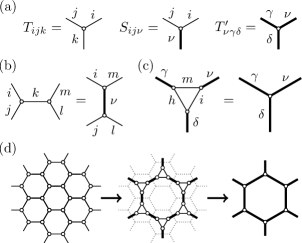
Rewiring: Graphically, let us represent the tensor at each point of the hexagonal lattice as a three-legged vertex as shown on the left of Fig. 1(a), and a contraction of an index between two tensors as a connection between two vertex legs. We use the convention that the order of indices in the tensor matches the counterclockwise ordering of the labels on the vertex legs. The rewiring step for a pair of neighboring tensors consists of reconnecting the bonds in the manner of Fig. 1(b), rewriting them as a contraction of two new tensors ,
| (2) |
The first two indices in the tensor run up to , but the third index runs up to . We shall distinguish these types of indices by a Greek letter label, and graphically depict them as thick legs [Fig. 1(a) center]. To see that such a rewiring is possible, let us introduce composite indices and , and write the tensor contraction on the left-hand side of Eq. (2) as a matrix . Then Eq. (2) becomes
| (3) |
or . We can find using the fact that , as can be checked using the cyclical symmetry of the tensors. Any symmetric matrix admits a variant of singular value decomposition known as Takagi factorization Takagi : , where is a unitary square matrix and is a diagonal matrix containing the singular values of . If is the th singular value (assumed ordered from largest to smallest with increasing ), then the elements of are given by . The resulting decomposition is not unique, because we can replace by , where is a complex orthogonal matrix (). However, we shall always use the given directly by the the Takagi factorization, so if the th singular value is nondegenerate, the th column of is uniquely determined up to a factor of . The rewiring procedure described above is applied globally to the entire hexagonal lattice as shown by the first arrow in Fig. 1(d), grouping the tensors into pairs, and replacing each pair by tensors.
Decimation: The second step in the renormalization procedure consists of tracing over the degrees of freedom in the triangular clusters that are formed after the rewiring. As illustrated in Fig. 1(c), each such cluster can be replaced by a single renormalized tensor ,
| (4) |
Introducing the notation for the matrix with elements at fixed , then the above equation has the form
| (5) |
It is clear from Eq. (5) that the renormalized tensor will be cyclically symmetric. Since the tensor is constructed from the unitary matrix , the elements of will in general be complex. The second arrow of Fig. 1(d) shows the decimation applied to every triangular cluster, and the result is a hexagonal lattice of tensors with the lattice spacing larger by a factor of compared to the original hexagonal lattice.
The renormalization-group transformation described so far is an exact mapping of one tensor network onto another, preserving the partition function . However, the renormalized tensors have a more complicated structure than the original ones, since the indices of run up to . If this procedure is repeated, the index range grows exponentially with iteration number, making numerical implementation impractical. This is analogous to the difficulty encountered when applying naive position-space renormalization to Hamiltonians on lattices, where the number of couplings in the Hamiltonian grows with each iteration. Some kind of approximate truncation is required to keep the complexity of the renormalized model bounded. In our case this truncation can be done in a straightforward and systematic fashion by setting an upper bound for the index range. Rather than use the full matrix to calculate , we use only the first columns, where . Using this truncated matrix, which we call , means that the rewiring step is implemented only approximately, . However, this is the best approximation possible, since the first columns of correspond to the largest singular values of . The decimation step of Eq. (4) is still carried out exactly, but with replaced by . The resulting tensor has indices that run up to .
III Renormalization-Group Flows and Thermodynamic Behavior of the Triangular Lattice Ising Model
In order to illustrate the nature of the renormalization-group flows resulting from the transformation outlined above and the methods by which thermodynamic information can be extracted from them, we turn now to a specific example: the triangular lattice ferromagnetic Ising model. This model is mapped onto a tensor network through a duality transformation, giving an equivalent partition function in terms of bond variables on a hexagonal lattice.LevinNave Each bond in this dual lattice has two states, or , corresponding to a bond between parallel or antiparallel Ising spins. These states respectively contribute energies and to the total Hamiltonian . The tensor for each lattice site has the form
| (6) |
where , and the factor multiplying the exponential is a projection operator that is equal to for allowed configurations of the bonds and otherwise. For simplicity we set , effectively measuring temperatures in units of . If the triangular lattice has sites, the dual hexagonal lattice has sites, and the partition function is a contraction of the site tensors.
Iterating the renormalization-group transformation, we consider renormalization-group flows in the space of tensor element amplitudes . For a cyclically symmetric tensor with index range , the maximum number of distinct elements is . After the first few iterations, the index range of the renormalized tensors reaches the cutoff and remains there, so that the flows in the subsequent steps are in a space with dimension . In this work we look at cutoffs in the range to , so the most complex flow space that we investigate is 4624-dimensional. A large number of the tensor elements are zero, corresponding to disallowed bond configurations, typically making up between 50-55% of the total in the later steps. The locations of the zero elements usually stay the same for a few steps at a time, but can shift abruptly during the flow. To minimize roundoff errors which can affect the results at later iterations, the singular value decomposition and matrix manipulations involved in TRG are all implemented at quadruple precision, using a customized version of the LAPACK library LAPACK .
Due to the contraction during the decimation step, the tensor elements tend to increase in magnitude rapidly with each iteration, which can lead to numerical problems. These are avoided similarly to the procedure used in global strong-coupling flows in position-space renormalization-group theory. The physics described by the tensor network is unaffected by an overall constant multiplying each element in the tensor. Thus at each step we factor out the absolute value of a nonzero element, for example , yielding a reduced tensor . The element is a convenient choice, since it remains nonzero throughout the renormalization-group flow. The renormalization-group transformation is then applied to the reduced tensor , giving a renormalized tensor . Let us denote as and as . The factorization and renormalization-group transformation are iterated, so at the th step we have a tensor . As we shall see below, with this added factorization step the elements of tend to finite limiting values as .
Additionally, keeping track of the factors during the flow, as in standard position-space renormalization-group theory, allows us to easily determine the free energy of the system in the thermodynamic limit.Nauenberg Defining , the partition function is a contraction of tensors , which we write schematically as . After a single renormalization-group step, this becomes . Thus after steps we find
| (7) |
The free energy per original site is then
| (8) |
As the elements of go to finite fixed values, and thus for large the second term on the right in Eq. (8) becomes negligible. So the final result for the free energy is . In practice the transformation is iterated for steps until the value of has converged to the limit within the desired numerical precision. Then .
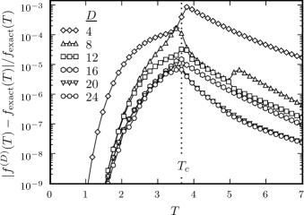
Even for small cutoffs , the results of this free energy calculation can be remarkably accurate, as seen in Fig. 2, which shows the relative error of , the free energy per site using cutoff , compared to the exact value . The latter is calculated by numerical evaluation of the integral solution in Ref. Wannier . Already at the TRG free energy is within 0.09% of the exact value at all temperatures, and is considerably more accurate than this away from the critical region near . As noted in Ref. LevinNave , the TRG method is expected to behave worst at criticality, and this is indeed what we see for all , with the relative error curves peaked near . Yet even here there is significant improvement as we go to larger cutoffs. At , the largest cutoff examined, the maximum error is 0.0007%. Overall, going from to we get an improvement between two and three orders of magnitude in the precision of the free energy result.
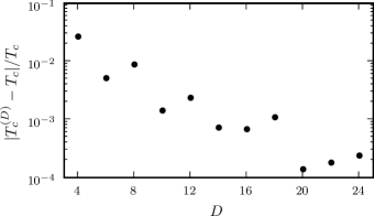
Further thermodynamic information can be gleaned by looking in detail at the behavior of the renormalization-group flows. The elements go to finite fixed values as , but unlike typical position-space renormalization-group transformations, there are no unique fixed points which act as a basins of attraction for the low- and high-temperature phases. Instead, at each different temperature the system flows to a different fixed point . However there is a way to distinguish the low- and high-temperature phases, since each flows to a different continuous surface of fixed points in the space of tensor elements. There is a boundary temperature , depending on the cutoff , such that for the flows tend to one fixed surface, while for they tend to the other. As becomes larger, gives a rapidly converging estimate of the exact critical temperature . Fig. 3 shows the relative error of compared to for various . While the decrease in error is not monotonic with , there is an overall trend which appears to be roughly exponential in the cutoff, so that the error at , , is two orders of magnitude smaller than at .
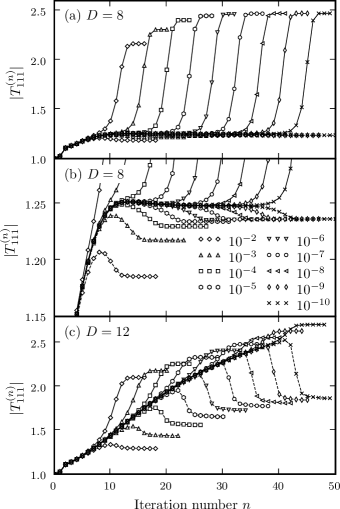
This segregation of the flows between two distinct fixed surfaces can be seen directly in Fig. 4, which plots one tensor element as a function of iteration number for and . The flows are shown for different values of , from to . There are two curves for each , one corresponding to , and the other to . The two curves stay close to one another for a number of iterations, but then veer off in opposite directions and reach different fixed values . These fixed values change continuously as is varied, as they map out a slice of the two fixed surfaces corresponding to the low- and high-temperature phases.
As gets smaller, there is an interesting difference in the flow behaviors of the and cases. For , as seen in Fig. 4(a) and in more detail in Fig. 4(b), the and curves are nearly horizontal before turning away to their respective fixed surfaces. This is true in fact for all the elements, since the flows are attracted to a unique critical fixed point, which we denote . The smaller the value of , the larger the number of iterations which are spent in the vicinity of before flowing to one of the fixed surfaces. Once we are in the vicinity of the critical fixed point, we can isolate it to high precision using a Newton-Raphson procedure. The analysis of the fixed point proceeds just as in a standard renormalization-group approach: we calculate a recursion matrix, whose eigenvalues can be related to the critical exponents of the system. To do this, let us denote the nonzero elements of , not related by cyclical symmetry, as through . In the case of , . For small perturbations away from the critical fixed point, the number and locations of these nonzero elements stay the same after a renormalization-group transformation, which allows us to numerically evaluate the recursion matrix . Writing the eigenvalues of in the form , , we find only one eigenvalue where , as expected at a critical fixed point. This relevant eigenvalue, which we denote , is related to the specific heat critical exponent by . For , , giving , which compare well to the exact values of and . We can check this result using an alternative approach, by calculating the specific heat from derivatives of the calculated free energy for small , and we find that the singularity in the specific heat agrees with the derived from the thermal eigenvalue of the recursion matrix.
| 4 | 3.73840 | 1.01543 | |
| 8 | 3.60873 | 1.01543 | |
| 12 | 3.64958 | ||
| 16 | 3.63847 | ||
| 20 | 3.64147 | ||
| 24 | 3.64183 | ||
| exact | 3.64096 | — | 1 |
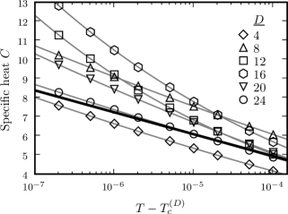
For the six values of the cutoff where we investigated the near-critical flows in detail, , we were able to isolate the critical fixed point for and , namely in 24- and 196-dimensional flow spaces. Despite the different dimensionalities of the flow spaces, both cases yielded the same eigenvalue , within the precision of 5 decimal places. Higher values of showed very different flow behaviors, as exemplified in Fig. 4(c) for . Here the and curves for do not stay nearly horizontal before diverging to the fixed surfaces: regardless of how small is made, the flows do not gravitate toward a unique critical fixed point, but map out a continuous spectrum of points which attract the flows before the two curves spread out. Using an arbitrary precision version of the TRG algorithm implemented in Mathematica, we checked values as small as without finding convergence toward a critical fixed point. Nevertheless, in these cases for we can still extract the critical behavior, by resorting to the alternative approach mentioned earlier: looking directly at the specific heat per site near as obtained from the numerical derivative of the calculated free energy. We plot within the high-temperature phase for various in Fig. 5, for between and . For each the data points are fit to a function , which provides an accurate description of the singularity, and the best-fit value of is used to determine the thermal eigenvalue . The results are listed in Table 1. For , , worse than our fixed-point determined values at or , but this value improves as is increased, reaching at . Moreover, as seen in Fig. 5, our calculated curve for nearly overlaps the exact as a function of , which diverges with a logarithmic singularity at the critical point.
IV Conclusion
In summary, we have seen that the flows of the tensor elements in the TRG transformation can be used to extract the phase diagram structure and critical behavior of a classical two-dimensional lattice Hamiltonian. For the triangular lattice Ising model, the low- and high-temperature phase regions are basins of attraction for two distinct surfaces of fixed points. The boundary between these basins defines a critical temperature , dependent on the TRG cutoff . At small cutoffs such as and 8, the flows near the boundary between the basins are controlled by a critical fixed point, while at higher the flows show more complicated behavior, never converging at a unique point. In the former case the thermal exponent is found from the eigenvalues of the recursion matrix at the critical fixed point, while in the latter we can deduce the exponent from the scaling of the calculated specific heat near . The free energy at all temperatures systematically converges to the exact Ising result with increasing , particularly fast away from the critical region. For the critical properties the improvement is not monotonic in , but both the critical temperature and the exponent tend toward the exact Ising values at larger cutoffs. With very modest computational effort, the TRG method provides an accurate portrait of global phase diagram characteristics. It thus warrants further study, both on applications to other two-dimensional lattice models, and possible generalization to systems with quenched randomness Falicov and/or higher spatial dimensions.
Acknowledgements.
This research was supported by the Scientific and Technical Research Council (TÜBİTAK) and by the Academy of Sciences of Turkey.References
- (1) M. Levin and C.P. Nave, arXiv:cond-mat/0611687.
- (2) Th. Niemeijer and J.M.J. van Leeuwen, Phys. Rev. Lett. 31, 1411 (1973).
- (3) A.A. Migdal, Zh. Eksp. Teor. Fiz. 69, 1457 (1975) [Sov. Phys. JETP 42, 743 (1976)].
- (4) L.P. Kadanoff, Ann. Phys. (N.Y.) 100, 359 (1976).
- (5) L.P. Kadanoff, Phys. Rev. Lett. 34, 1005 (1975).
- (6) L.P. Kadanoff, A. Houghton, and M.C. Yalabık, J. Stat. Phys. 14, 171 (1976).
- (7) A.N. Berker and M. Wortis, Phys. Rev. B 14, 4946 (1976).
- (8) I. Markov and Y. Shi, arXiv:quant-ph/0511069.
- (9) Y. Shi, L. Duan, and G. Vidal, Phys. Rev. A 74, 022320 (2006).
- (10) T. Takagi, Japan. J. Math. 1, 83 (1925).
- (11) E. Anderson et. al., LAPACK Users’ Guide (SIAM, Philadelphia, PA, 1999), 3rd ed.
- (12) M. Nauenberg, J. Math. Phys. 16, 703 (1975).
- (13) G.H. Wannier, Phys. Rev. 79, 357 (1950); erratum: Phys. Rev. B 7, 5017 (1973).
- (14) A. Falicov, A.N. Berker, and S.R. McKay, Phys. Rev. B 51, 8266 (1995).