Shape and orientation of stellar velocity ellipsoids in spiral galaxies

Abstract

We present a numerical study of the properties of the stellar velocity distribution in stellar discs which have developed a saturated, two-armed spiral structure. We follow the growth of the spiral structure deeply into the non-linear regime by solving the Boltzmann moment equations up to second order. By adopting the thin-disc approximation, we restrict our study of the stellar velocity distribution to the plane of the stellar disc. We find that the outer (convex) edges of stellar spiral arms are characterized by peculiar properties of the stellar velocity ellipsoids, which make them distinct from most other galactic regions. In particular, the ratio $\sigma_{1}:\sigma_{2}$ of the smallest versus largest principal axes of the stellar velocity ellipsoid can become abnormally small (as compared to the rest of the disc) near the outer edges of spiral arms. Moreover, the epicycle approximation fails to reproduce the ratio $\sigma_{\phi\phi}:\sigma_{rr}$ of the tangential versus radial velocity dispersions in these regions. These peculiar properties of the stellar velocity distribution are caused by large-scale non-circular motions of stars, which in turn are triggered by the non-axisymmetric gravitational field of stellar spiral arms.

The magnitude of the vertex deviation appears to correlate globally with the amplitude of the spiral stellar density perturbations. However, locally there is no simple correlation between the vertex deviation and the density perturbations. In particular, the local vertex deviation does not correlate with the local gravitational potential and shows only a weak correlation with the local gravitational potential gradient. We find that the local vertex deviation correlates best with the spatial gradients of mean stellar velocities, in particular with the radial gradient of the mean radial velocity.

1 Introduction

Already since the end of the nineteenth century studies of stellar kinematics in the solar neighbourhood revealed that the velocity distribution of stars in galactic discs is non-isotropic (Kobold kobold90 1890). An early interpretation by Kapteyn (kapteyn05 1905) and Eddington (eddington06 1906) invoked a superposition of (isotropic) stellar streams with different mean velocities, by this creating an anisotropic velocity distribution. However, an alternative interpretation by Schwarzschild (schwarzschild07 1907) became the general framework for describing the local velocity distribution of stars of equal age, though a contamination by stellar streams is still considered to be important for a proper analysis of velocity data. The Schwarzschild distribution is based on a single but anisotropic ellipsoidal distribution function. It is characterized by a Gaussian distribution in all three directions $U$ (radial $r$), $V$ (tangential $\phi$) and $W$ (vertical $z$) in velocity space, but with different velocity dispersions $\sigma_{rr}$, $\sigma_{\phi\phi}$, and $\sigma_{zz}$. In general, the velocity distribution is described by a velocity dispersion tensor

$$\sigma^{2}_{ij}\equiv\overline{(v_{i}-\bar{v_{i}})(v_{j}-\bar{v_{j}})},$$ (1)

where $i$ and $j$ denote the different coordinate directions, i.e. radial ($r$), azimuthal ($\phi$) and vertical ($z$) direction and $v_{i}$ gives the corresponding velocity. The bar denotes local averaging over velocity spacee emphasize that our definition of the velocity dispersion tensor is different from the definition of e.g. Kuijken & Tremaine (KT 1994) who do not use a square mark. Hence, our $\sigma^{2}_{ij}$ is equivalent to Kuijken & Tremaine’s $\sigma_{ij}$. . The principal axes of this tensor form an imaginary surface that is called the velocity ellipsoid. The principal axes of the velocity ellipsoid need not to be aligned with the coordinate axes. In that case, the vertex deviation $l_{\rm v}$ (which is defined as the angle between the direction in velocity space pointing from the Sun to the Galactic centre and the direction of the $\sigma_{ij}$ major principal axis) does not vanish.

The general trend for the velocity dispersions is that the radial velocity dispersions are the largest and the vertical velocity dispersions are the smallest among stars of same age and stellar type. This trend holds when dispersions are averaged locally, i.e. in the solar neighbourhood (Dehnen & Binney Dehnen 1998), or globally over the entire galactic discs. For instance, the ratio $\sigma_{rr}:\sigma_{\phi\phi}:\sigma_{zz}$ of the radial, tangential, and vertical stellar velocity dispersions in the disc of NGC 488 is approximately $1:0.8:0.7$ (Gerssen et al. Gerssen 1997).

In the case of stationary, axisymmetric systems and appropriate distribution functions (DF) the velocity ellipsoid is aligned with the coordinate axes. If the stellar orbits are nearly circular (i.e. with small radial amplitudes with respect to the guiding centre), then the Oort ratio $X^{2}\equiv\sigma^{2}_{\phi\phi}:\sigma^{2}_{rr}$ of tangential versus radial stellar velocity dispersions can be calculated in zero order approximation within the epicyclic theory to be $X^{2}_{\rm ep}=-B/(A-B)$, where $A$ and $B$ are the usual Oort constants. For a flat rotation curve one gets $X^{2}_{\rm ep}=1/2$. More realistic axisymmetric distribution functions give first order corrections, which yield values of $X^{2}=0.59$ (or 0.66) for the solar vicinity (Kuijken & Tremaine kuijken91 1991, hereafter KT91). Clearly, these values exceed those predicted by the epicycle approximation. On the other hand, observations in the Milky Way (MW) give lower (mean) values around $X^{2}=0.42-0.45$, which are substantially below the epicycle value $X^{2}_{\rm ep}=1/2$ (Kerr & Lynden-Bell kerr86 1986; Ratnatunga & Upgren ratnatunga97 1997). The exact reason for this discrepancy is still unknown. It might stem from a DF asymmetric in $v_{\phi}$ (KT91) or from invalid assumptions, i.e. a violation of stationarity or axisymmetry.

Additionally, non-vanishing vertex deviations were found in the solar vicinity in many studies (e.g. Wielen wielen74 1974, Mayor mayor72 1972, Ratnatunga & Upgren ratnatunga97 1997). These vertex deviations could be explained by spiral structures (Mayor mayor70 1970, Yuan yuan71 1971), by this supporting the importance of non-axisymmetry of the underlying gravitational potential. Moreover, a clear relation between $l_{\rm v}$ and $\sigma_{rr}$ has been found. For smaller velocity dispersions larger vertex deviations have been measured, e.g. for a radial velocity dispersion of about 15 km s^-1 one gets a vertex deviation of $25^{\circ}-30^{\circ}$ (Wielen wielen74 1974).

A major step in analysing the local stellar velocity space was the astrometric satellite mission Hipparcos (ESA esa97 1997). Earlier results concerning the general behaviour of the velocity ellipsoid, e.g. the dependence of the dispersions or the vertex deviations as a function of $B-V$ were corroborated (Dehnen & Binney Dehnen 1998, Bienaymé bienayme99 1999, Hogg et al. hogg05 2005). Moreover, the more numerous known proper motions allowed for a detailed mapping of the velocity space in the solar vicinity. It turned out that the local velocity distribution of stars exhibits a lot of substructure (Dehnen dehnen98 1998, Alcobé & Cubarsi alcobe05 2005). For example, two major peaks in the velocity distribution were found where the smaller secondary peak is well detached by at least 30 km s^-1 from the main peak (the “u anomaly”). Dehnen (dehnen00 1999) attributed this bimodality to the perturbation exerted by the Galactic bar assuming that its outer Lindblad resonance (OLR) is close to the Sun. Mühlbauer & Dehnen (muehlbauer03 2003) showed that a central bar can also explain vertex deviations of about 10^∘, and Oort ratios below 1/2. Recent investigations about the influence of the Galactic bar on Oort’s $C$ constant corroborated these results and gave stronger limits on the bar’s properties (Minchev et al. minchev07b 2007). Minchev & Quillen (minchev07a 2007) showed also that a stationary spiral cannot reproduce the ”u anomaly”. Though less likely, an alternative interpretation of the bimodality as a result of non-stationary spiral arms cannot be ruled out completely.

In general, a non-axisymmetric gravitational potential might lead to both, a misalignment of the velocity ellipsoid and an additional correction of the velocity dispersion ratio $X^{2}$ with respect to the value predicted by the epicycle approximation. In the case of spiral perturbations, this conclusion was made e.g. by Mayor (mayor70 1970, for a review of different mechanisms see KT91) and numerically confirmed recently by Vorobyov & Theis (VT 2006, hereafter VT06). Using linear perturbation analysis KT91 studied different discs subject to oscillating perturbations (like a rotating bar or a spiral) or subject to a static non-axisymmetric dark matter halo. In the case of large-scale oscillating perturbations the predicted vertex deviations oscillate, too. Once the axisymmetric background gravitational potential and the pattern speed of the perturbation are fixed, its amplitude depends in a complex way only on the perturbed mean velocity and its spatial gradient. For a static elliptic potential Kuijken & Tremaine (KT 1994) showed that the observed mean kinematic data ($X^{2}$ and $l_{\rm v}$) can be explained, if the ellipticity of the disc is about $q\approx 0.88$ and the Sun’s location is near to the minor axis of the corresponding potential. It is remarkable that the correction terms introduced by the non-axisymmetry are negative (i.e. in agreement with the observations in the Milky Way), whereas the higher order terms derived from a more realistic axisymmetric DF are positive. Similarly, Blitz & Spergel (blitz91 1991) argued for a slowly rotating mildly triaxial Galactic potential, resulting in an outward motion of 14 km s^-1 of the LSR and a vertex deviation of 10^∘.

However, it is not clear if the non-axisymmetric gravitational field is entirely responsible for the observed vertex deviation. The existence of moving groups of stars was shown to produce large vertex deviations (Binney & Merrifield BM 1998). The situation may become even more complicated because moving groups of stars may in turn be caused by the non-axisymmetric gravitational field of spiral arms. Therefore, a detailed numerical study of the vertex deviation in spiral galaxies is necessary.

In this paper, we present the stellar hydrodynamics simulations of linear and non-linear stages of the spiral structure formation in stellar discs by solving numerically the Boltzmann moment equations up to second order in the thin-disc approximation. In contrast to linear stability analyses, we follow the growth of the spiral structure self-consistently. Compared to $N$-body simulations, we have the advantage that we can follow the spiral structure formation from a very low perturbation level deeply into the non-linear regime. The former is usually hardly accessible by self-consistent $N$-body simulations due to particle noise. We study the local evolution of the velocity dispersion tensor in the plane of the disc, which includes the anisotropy ($X^{2}$), the ratio of the smallest versus largest principal axes of the stellar velocity ellipsoid, and the vertex deviation ($l_{\rm v}$).

The paper is organized as follows. In Section 2 we give a short description of the numerical code. The model galaxy and initial conditions are described in Section 3. The physical explanation for the growth of the spiral structure in our model disc is given in Section 4. The shape and orientation of stellar velocity ellipsoids is studied in Section 5. In Section 6 we discuss the applicability of the epicycle approximation and possible causes of the vertex deviation in spiral galaxies. The summary and conclusions are given in Section 7.

2 The method and numerical code

Stars are collisionless objects that move on orbits determined by the large-scale gravitational potential. An exact description of such a system requires the solution of the collisionless Boltzmann equation for the distribution function of stars $f({\mbox{\boldmath$r$}},{\mbox{\boldmath$v$}},t)$ in the phase space ($\mbox{\boldmath$r$},\mbox{\boldmath$v$}$). A general solution of the Boltzmann equation, which is defined in a six-dimensional position and momentum phase space, is usually prohibited due to the large computational expense. However, taking moments of the Boltzmann equation in velocity space turns out to yield a set of equations that is numerically tractable.

In our recent paper (VT06) we presented the BEADS-2D code that is designed to study the dynamics of stellar discs in galaxies. The BEADS-2D code is a finite-difference numerical code that solves the Boltzmann moment equations up to second order in the thin-disc approximation on a polar grid ($r,\phi$). More specifically, the BEADS-2D code solves for the stellar surface density $\Sigma$, mean radial and tangential stellar velocities $u_{r}$ and $u_{\phi}$, and stellar velocity dispersion tensor. The latter includes the squared radial and tangential stellar velocity dispersions $\sigma^{2}_{rr}$ and $\sigma^{2}_{\phi\phi}$, respectively, and the mixed velocity dispersion $\sigma^{2}_{r\phi}$. We close the system of Boltzmann moment equations by adopting the zero-heat-flux approximation. This approximation is equivalent to assuming the absence of any heat transfer in the classic fluid dynamics approach. The BEADS-2D code has shown a good agreement with the predictions of linear stability analysis of self-gravitating stellar discs (e.g. Polyachenko et al. Polyachenko 1997, Bertin et al. bertin00 2000).

The use of the Boltzmann moment equation approach allows us to study non-isotropic stellar systems, in particular, the shape and orientation of stellar velocity ellipsoids within the discs of spiral galaxies. The BEADS-2D code directly evolves observable quantities, and it can follow their evolution over many e-folding times starting from arbitrary small perturbations. These properties make the stellar hydrodynamics approach advantageous over the more common N-body codes which, however, suffer strongly from particle noise. Presently, the BEADS-2D code is limited by its two-dimensionality (the thin-disc approximation) but a fully three-dimensional implementation is currently under development. The interested reader is referred to VT06 for details. In the current simulations, the numerical resolution has $512\times 512$ grid zones that are equally spaced in the $\phi$-direction and logarithmically spaced in the $r$-direction. The inner and outer reflecting boundaries are at 0.2 kpc and 35 kpc, respectively. We extend the outer computational boundary far enough to ensure a good radial resolution in the region of interest within the inner 20 kpc. For instance, the radial resolution at 1 kpc and 20 kpc is approximately 10 pc and 150 pc, respectively.

3 Model galaxy and initial conditions

In this paper we study the influence of a spiral gravitational field on the properties of stellar velocity ellipsoids within the disc of a spiral galaxy. Our model galaxy consists of a thin, self-gravitating stellar disc embedded in a static dark matter halo. The initial surface density of stars is axisymmetric and is distributed exponentially according to

$$\Sigma(r)=\Sigma_{0}\exp(-r/r_{\rm d}),$$ (2)

with a radial scale length $r_{\rm d}$ of 4 kpc. The central surface density $\Sigma_{0}$ is set to $10^{3}~{}M_{\odot}$ pc^-2. We note that the densities of stellar discs are indeed found to decay exponentially with distance, with a characteristic scale length increasing from $2-3$ kpc for the early type galaxies to $4-5$ kpc in the late type galaxies (Freeman freeman 1970).

The gravitational potential $\Phi_{\rm disc}$ of the stellar disc is calculated by

$$\Phi_{\rm disc}(r,\phi) = -G\int_{0}^{\infty}r^{\prime}dr^{\prime}$$ (3)

$$\times\int_{0}^{2\pi}\frac{\Sigma(r^{\prime},\phi^{\prime})d\phi^{\prime}}{\sqrt{{r^{\prime}}^{2}+r^{2}-2rr^{\prime}\cos(\phi^{\prime}-\phi)}}\,.$$

This sum is calculated using a FFT technique that applies the 2D Fourier convolution theorem for polar coordinates (Binney & Tremaine BT 1987, Sect. 2.8).

The initial mean rotational (tangential) velocity of stars in the disc is chosen according to

$$u_{\phi}=u_{\infty}\cdot\left(\frac{r}{r_{\rm flat}}\right)\cdot\frac{1}{\displaystyle\left[1+\left(\frac{r}{r_{\rm flat}}\right)^{n_{v}}\right]^{\displaystyle\frac{1}{n_{v}}}}\,\,.$$ (4)

The transition radius between the inner region of rigid rotation and a flat rotation in the outer part is given by $r_{\rm flat}$, which we set to 3 kpc. The smoothness of the transition is controlled by the parameter $n_{v}$, set to 3. The velocity at infinity, $u_{\infty}$, is set to 208 km s^-1. The resulting rotation curve is shown in Fig. 1 by the solid line. The initial mean radial velocity of the stars $u_{r}$ is set to zero.

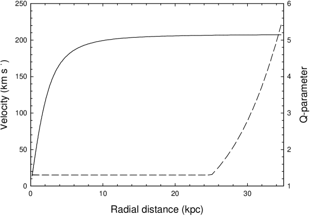
Figure 1: Rotation curve (solid line) and radial distribution of the Toomre $Q_{s}$ parameter (dashed line) in the model stellar disc.

The radial component of the velocity dispersion is obtained from the relation $\sigma_{rr}=3.36\,Q_{\rm s}\,G\,\Sigma/\kappa$ for a given value of the Toomre parameter $Q_{\rm s}$. Here, $\kappa$ is the epicycle frequency. We assume that throughout most of the disc $Q_{\rm s}$ is constant and equal 1.3 but is steeply increasing with radius at $r>25$ kpc. The initial radial distribution of $Q_{\rm s}$ is shown in Fig. 1 by the dashed line. The tangential component of the velocity dispersion $\sigma_{\phi\phi}$ is determined adopting the epicycle approximation, in which the following relation between $\sigma^{2}_{\phi\phi}$ and $\sigma^{2}_{rr}$ holds (Binney & Tremaine BT 1987, p. 125):

$$\sigma_{\phi\phi}^{2}=\sigma_{rr}^{2}\cdot{1\over 2}\left({r\over u_{\rm c}}{du_{\rm c}\over dr}+1\right),$$ (5)

where $u_{\rm c}$ is the circular speed, i.e. the speed of a hypothetical star in a circular orbit determined exclusively by the gravitational potential. The value of $u_{\rm c}$ is yet undefined (since the gravitational potential of the dark matter halo is yet undefined) and we substitute the circular speed with the initial rotation velocity of stars $u_{\phi}$. We emphasize that equation (5) is valid only for stars on nearly circular orbits. We discuss the practical application of the epicycle approximation to spiral galaxies in section 5.1. The mixed velocity dispersion $\sigma^{2}_{r\phi}$ is initially set to zero.

Once the rotation curve and the radial profiles of the stellar surface density and velocity dispersions are fixed, the dark matter halo potential $\Phi_{\rm halo}$ can be derived from the following steady-state momentum equation (see eq. (4) in VT06)

$$\Sigma\left({\partial\Phi_{\rm disc}\over\partial r}+{\partial\Phi_{\rm halo}\over\partial r}\right)-{\Sigma\sigma_{\phi\phi}^{2}\over r}-{\Sigma u_{\phi}^{2}\over r}+{1\over r}{\partial\over\partial r}\left(r\Sigma\sigma_{rr}^{2}\right)=0$$ (6)

4 Development of a spiral structure

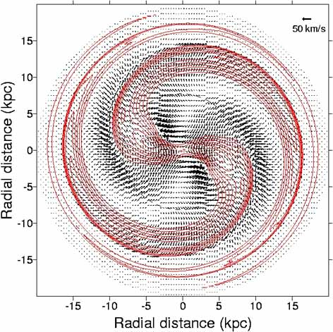
Figure 2: Contour lines of the positive stellar density perturbation relative to the initial axisymmetric density distribution at $t=1.6\,\,\mathrm{Gyr}$. The maximum and minimum contour levels are 0.8 and 0.1, respectively and the step is 0.1. The residual stellar velocity field in km s^-1 is superimposed on the contour lines (see the text for details).

When starting our simulations we add a small random perturbation to the initially axisymmetric surface density distribution of stars. The relative amplitude of the perturbation in each computational zone is less than or equal to $10^{-5}$. Since the model stellar disc is characterized by $Q_{\rm s}=1.3$, it becomes vigorously unstable to the growth of non-axisymmetric gravitational instabilities. We find that the positive density perturbation relative to the initial density distribution in the disc can be a good tracer for the spiral structure. Hence, we define the relative stellar density perturbation as

$$\zeta(r,\phi)={\Sigma(r,\phi)-\Sigma_{\rm in}(r)\over\Sigma_{\rm in}(r)},$$ (7)

where $\Sigma_{\rm in}(r)$ is the initial axisymmetric stellar density distribution in the disc and $\Sigma(r,\phi)$ is the current stellar density distribution. The positive values of $\zeta(r,\phi)$ at $t=1.6$ Gyr are plotted in Fig. 2 by the red contour lines. The maximum and minimum contour levels correspond to the relative perturbations of $0.8$ and $0.1$, respectively, and the step is $0.1$. The position of corotation at approximately 8.5 kpc is shown by the dashed circle. The stellar disc has clearly developed a two-armed spiral structure and a central bar. A movie showing the time development of the spiral structure can be found at http://www.univie.ac.at/theis/swing_VT07.avi. Snapshots from different stages of the evolution have also been presented by VT06 for a similar model stellar disc.

In our numerical simulations, the bar forms within the 4:1 ultraharmonic resonance (UHR), which is located at approximately 4.5 kpc. At the end of the bar, a slightly weaker spiral structure emerges almost perpendicularly to the bar. Such transitions of bars to spirals are not uncommon (e.g. NGC 1672 or NGC 3513). Radially, our spiral arms reach up to the OLR ($\sim$ 15 kpc). Azimuthally, they cover an angle of about $\pi$ where they start to fade out. The strongest gradients in the stellar density are found near the outer (convex) edges of the spiral arms. The pattern speeds of the bar and the spiral structure are identical. Based on orbital analysis, Kaufmann & Contopoulos (kaufmann96 1996) identified the UHR as a transition region between a bar and spiral features for systems characterized by a single pattern speed for both the bar and the spiral. Recently, Patsis (patsis06 2006) has shown that such a coupling is related to chaotic orbits that resemble for a long time the 4:1-resonance orbital behaviour. We note that beyound 10 kpc our spiral arms are very tightly wound due to the decreasing pitch angle. This is in contrast to logarithmic spirals observed in most spiral galaxies. This inconsistency may be caused by the presence of the OLR in our model galaxy where spiral arms tend to converge to a resonant ring. We also emphasize that the amplitude of the spiral stellar density perturbation is quickly decreasing as one approaches the OLR, which makes it difficult to observe the stellar spirals near the OLR in real galaxies.

The non-axisymmetric gravitational field of the spiral arms and the bar perturbs stellar orbits. To better illustrate this effect, we plot in Fig. 2 the residual velocity field of stars at $t=1.6$ Gyr. The residual velocities are obtained by subtracting the initial mean rotation velocities of stars (shown in Fig. 1) from the current mean velocities. Noticeable large-scale perturbations to the initially axisymmetric flow of stars are seen between the spiral arms and near the bar. The flow pattern near the convex edges of spiral arms (and outside corotation) is particularly interesting. The non-axisymmetric gravitational field of the spiral arm creates two counterpointed large-scale streams of stars, which merge near the convex edge of the spiral into a narrow retrograde stellar stream. A similar phenomenon, though less apparent, is seen near the inner edges of the bar where two merging streams of stars produce a strongly perturbed velocity pattern. The regions with merging stellar streams occupy only a small portion of the stellar disc. However, as we will see in the next section, these regions are characterised by the most pronounced influence of the non-axisymmetric gravitational field on the shape and orientation of stellar velocity ellipsoids.

As demonstrated recently in VT06, the most likely physical interpretation for the growth of a spiral structure in our model disc is swing amplification. Amplification occurs when any leading spiral disturbance unwinds into a trailing one due to differential rotation (Goldreich & Lyndell-Bell GLB 1965, Toomre Toomre 1981, Athanassoula athanassoula84 1984, and others). According to Julian & Toomre (JT 1966), the gain of the swing amplifier in a stellar disc with $Q_{\rm s}=1.2$ and a flat rotation curve is the largest when $0.5\mathrel{\hbox{\hbox to0.0pt{\hbox{\lower 4.0pt\hbox{$\sim$}}\hss}\hbox{$<$}}}\tilde{X}\mathrel{\hbox{\hbox to0.0pt{\hbox{\lower 4.0pt\hbox{$\sim$}}\hss}\hbox{$<$}}}2.5$. The latter quantity is defined as $\tilde{X}\equiv\lambda/\lambda_{\rm cr}$, where $\lambda\equiv 2\pi r/m$ is the circumferential wavelength of an $m$-armed spiral disturbance and $\lambda_{\rm cr}\equiv 4\pi^{2}G\Sigma/\kappa^{2}$ is the longest unstable wavelength in a cold disc. Generally speaking, swing amplification is most efficient when $\lambda\approx\lambda_{\rm cr}$. At $\lambda\gg\lambda_{\rm cr}$ and $\lambda\ll\lambda_{\rm cr}$, the swing amplifier is strongly moderated by local shear and random motion of stars, respectively.

The top panel of Fig. 3 shows the radial profiles of the $\tilde{X}$-parameter for the $m=1$ (solid line), $m=2$ (dashed line), $m=3$ (dash-dotted line), and $m=4$ (dash-dot-dotted line) spiral perturbations. The region of maximum swing amplification is bound by the two horizontal dotted lines. It can be clearly seen that the $m=1$ perturbations are swing amplified in the inner 5 kpc, whereas the $m=2$ perturbations are swing amplified over a much larger area between 1 kpc and 12 kpc. Consequently, the $m=2$ perturbations are expected to engage more stellar mass into the amplification process than the $m=1$ perturbations. Hence, it is natural to conclude that the $m=2$ density perturbations should grow faster and ultimately surpass the $m=1$ perturbations.

Why then does our model stellar disc develop a two-armed global spiral pattern rather than a three-armed or any other multi-armed pattern? Indeed, higher order perturbations are also swing amplified over a considerable area of the disc, as Fig. 3 (top panel) demonstrates. The answer is that swing amplification needs a feedback mechanism that can constantly feed a disc with leading spiral disturbances. The trailing short-wavelength disturbances may propagate through the centre and emerge on the other side as leading ones, thus providing a feedback for the swing amplifier. Figure 4 in VT06 and the mentioned movie nicely illustrate this phenomenon. However, the propagation of stellar disturbances through the disc centre is possible if there is no inner Lindblad resonance (ILR) or if the waves are reflected before reaching the ILR. A $Q$-barrier allows for such a reflection of propagating waves (e.g. Athanassoula athanassoula84 1984) but it is absent in the inner region of our model disc (see Fig. 1).

To determine the position of Lindblad resonances $m(\Omega_{\rm p}-\Omega)=\pm\kappa$, we plot in the bottom panel of Fig. 3 the radial profiles of $\Omega$ and $\Omega\pm\kappa/m$ for the initial axisymmetric stellar disc and two global spiral modes $m=2$ and $m=3$. The angular velocity of the two-armed global spiral pattern (see next section) is determined from both visual and numerical estimates to be $\Omega_{\rm p}=23\pm 1$ km s^-1 kpc^-1. This value is plotted by the dotted line in the bottom panel of Fig. 3. It is clearly seen that the $m=2$ disturbances have no inner Lindblad resonance, $\Omega-\kappa/2<\Omega_{\rm p}$ at all radii. On the other hand, the $m=3$ disturbances have the inner Lindblad resonance near the disc centre, $\Omega-\kappa/3\approx\Omega_{\rm p}$ in the inner 2 kpc. This prevents the $m=3$ (and any higher order) disturbances from propagating through the disc centre, which terminates the feedback mechanism for the swing amplifier for these modes. We find that this mechanism works nicely in stellar discs with other radial configurations of the $\tilde{X}$-parameter and pattern angular velocities $\Omega_{\rm p}$ and can allow for the dominant growth of $m=1$, $m=3$, and other higher order global spiral modes. The results of this study will be presented in a future paper.

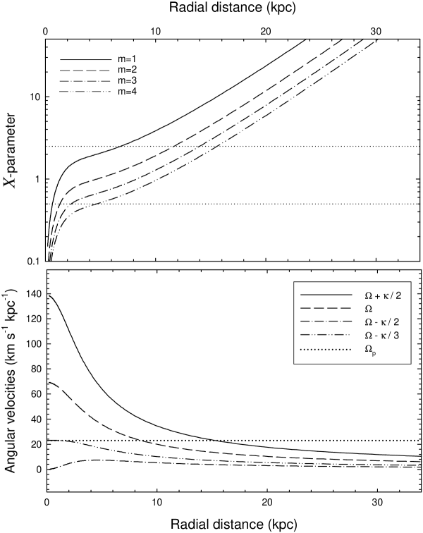
Figure 3: Top panel. Radial profiles of the $\tilde{X}$-parameter for the $m=1$ (solid line), $m=2$ (dashed line), $m=3$ (dash-dotted line), and $m=4$ (dash-dot-dotted line) spiral perturbations. Two horizontal dotted lines delimit the region of maximum swing amplification. Bottom panel. Radial profiles of the angular velocity of stars $\Omega$ and $\Omega\pm\kappa/m$ for the initial axisymmetric stellar disc and two spiral modes $m=2$, and $m=3$. The angular velocity of the spiral pattern $\Omega_{\rm p}$ is plotted by the dotted line. There is no inner Lindblad resonance for the $m=2$ mode, whereas the $m=3$ mode has the inner Lindblad resonance near the disc centre.

5 The shape and orientation of stellar velocity ellipsoids

5.1 Stellar velocity dispersions and spiral structure

Despite more exotic means of galactic disc heating there are currently two known mechanisms involving spirals as the heating agents. These are transient spiral stellar density waves (e.g. Wielen Wielen 1977, Carlberg & Sellwood CS 1985, Jenkins & Binney JB 1990, De Simone et al. DeSimone 2004) and multiple spiral stellar density waves (Minchev & Quillen Minchev06 2006). The latter mechanism involves two sets of steady state spiral structure moving at different pattern speeds. We note that a single steady state spiral structure as defined in e.g. Lin et al. (Lin 1969) does not heat stellar discs.

In this section, we focus on the effect that the non-axisymmetric gravitational field of a swing amplified spiral structure may have on the spatial distribution of stellar velocity dispersions within a stellar disc. Figures 4a and 4b show the spatial distribution of the radial and tangential stellar velocity dispersions, respectively, at $t=1.6$ Gyr. A two-armed spiral structure and a bar are apparent in the spatial distribution of $\sigma_{rr}$ and $\sigma_{\phi\phi}$. To better illustrate this phenomenon, we plot in Figs 4c and 4d the stellar velocity dispersion perturbations relative to their initial values at $t=0$ Gyr. More specifically, Fig. 4c shows the relative perturbations in the radial velocity dispersion calculated as $(\sigma_{rr}-\sigma^{0}_{rr})/\sigma^{0}_{rr}$, where $\sigma^{0}_{rr}$ is the initial radial velocity dispersion and $\sigma_{rr}$ is the model’s known radial velocity dispersion at $t=1.6$ Gyr. To avoid confusions, we note that $\sigma_{rr}$ and $\sigma_{\phi\phi}$ are measured in km s^-1 throughout the paper. Figure 4d shows the relative perturbations in the tangential velocity dispersion $\sigma_{\phi\phi}$ calculated in a similar manner. The positive and negative perturbations are plotted with the shadows of red and blue, respectively. The contour lines of the positive stellar density perturbations are shown for convenience. Figure 4 clearly demonstrates that the non-axisymmetric gravitational field has a pronounced global influence on the spatial distribution of stellar velocity dispersions in the disc. The most distinctive feature in Fig. 4 is that the positive (and negative) relative perturbations in density and both stellar velocity dispersions correlate spatially, suggesting a causal link. We emphasize that the largest spatial gradients in both velocity dispersions (and in the stellar surface density) are found near the outer (convex) edges of the spiral arms. As we will see in Section 6.1, this may cause a severe failure of the epicycle approximation in these regions.

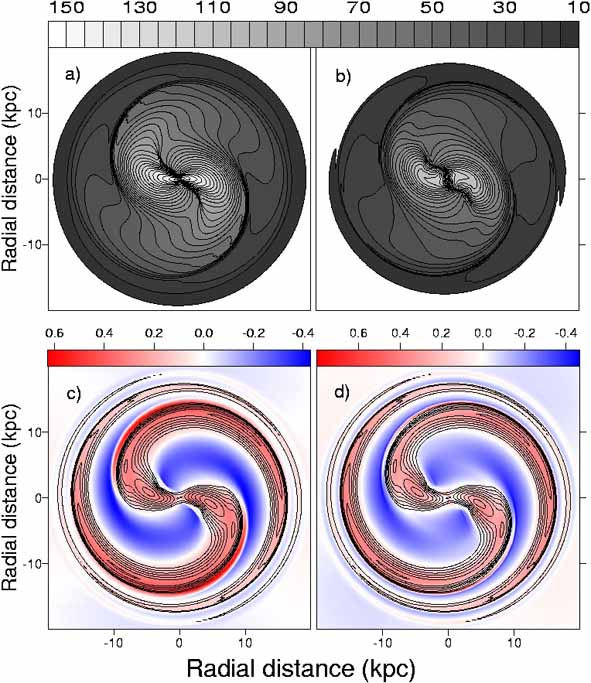
Figure 4: Spatial distribution of (a) the radial and (b) tangential stellar velocity dispersions at $t=1.6$ Gyr. The scale bar is in km s^-1. The spiral structure is clearly seen in the distribution of both velocity dispersions. Perturbations in (c) the radial and (d) tangential velocity dispersions at $t=1.6$ Gyr relative to their initial values. The contour lines of the positive stellar density perturbations are shown in (c) and (d) for convenience (see Fig. 2 for details). Note that the positive relative perturbations in the velocity dispersions correlate spatially with the positive relative density perturbations shown in Fig. 2.

5.2 The shape of stellar velocity ellipsoids

In contrast to gaseous discs, stellar discs are essentially non-isotropic. This means that the local properties of stars, such as mean velocities, are determined by the velocity dispersion tensor $\sigma$ rather than by an isotropic pressure. The tensor $\sigma$ is often non-diagonal in the local coordinate system ($r,\phi,z$). The principal axes of a diagonalized velocity dispersion tensor form an imaginary ellipsoidal surface that is called the velocity ellipsoid. The available measurements in the solar vicinity indicate that the ratio $\sigma_{1}:\sigma_{2}$ of the smallest versus largest principal axes of the stellar velocity ellipsoid in the disc plane does not vary significantly with the $B-V$ colour. According to Dehnen & Binney (Dehnen 1998), the axis ratio $\sigma_{1}:\sigma_{2}$ is approximately $0.6\pm 0.1$ for stars with $-0.2\leq B-V\leq 0.7$. To avoid confusions, we note that throughout the paper $\sigma_{1}$ and $\sigma_{2}$ are measured in km s^-1. The $B-V$ colour of an ensemble of stars may be considered as a rough estimate of their mean age. A weak sensitivity of the axis ratio $\sigma_{1}:\sigma_{2}$ to the age of stellar populations is intriguing since the principal axes of velocity ellipsoids (when considered separately) are indeed age sensitive and show a noticeable (a factor of two) increase along increasing $B-V$ colours (Dehnen & Binney Dehnen 1998).

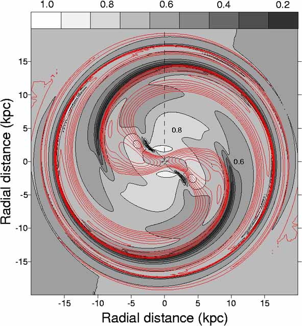
Figure 5: Contour map of the positive stellar density perturbations (red lines) superimposed on the ratio $\sigma_{1}:\sigma_{2}$ of smallest versus largest principal axes of stellar velocity ellipsoids at $t=1.6$ Gyr. Note abnormally small values of $\sigma_{1}:\sigma_{2}$ at the outer (convex) edges of spiral arms.

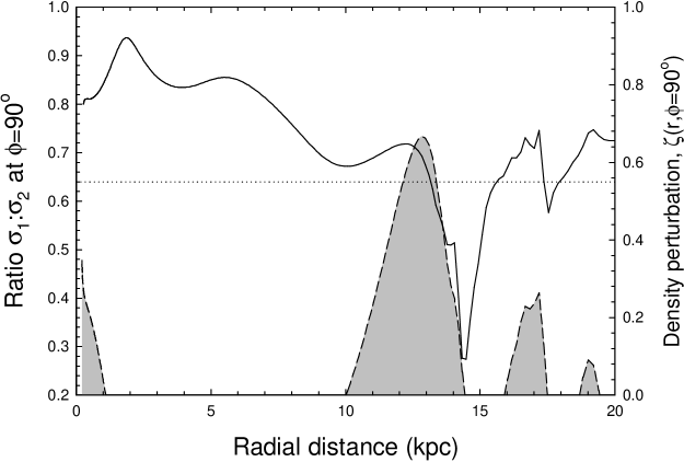
Figure 6: Radial profiles of the ratio $\sigma_{1}:\sigma_{2}$ (solid line) and positive relative perturbation in the stellar surface density (dashed line) obtained from Fig. 5 by taking a radial cut at the azimuthal angle $\phi=90^{\circ}$. Note that $\sigma_{1}:\sigma_{2}$ attains local minima just at the outer (convex) edges of spiral arms.

If the axis ratio $\sigma_{1}:\sigma_{2}$ is indeed only weakly sensitive to the age of stellar populations, it would be interesting to determine other phenomena that could possibly affect the values of $\sigma_{1}:\sigma_{2}$. In this section, we consider the effect that the non-axisymmetric gravitational field of the spiral arms and the bar may have on the shape of stellar velocity ellipsoids within the disc of our model galaxy. Figure 5 shows the contour plot of the positive stellar density perturbation (red lines) superimposed on the grey-scale map of $\sigma_{1}:\sigma_{2}$ in the disc at $t=1.6$ Gyr. It is evident that the central 5 kpc are characterized by $\sigma_{1}:\sigma_{2}\approx 0.8-0.9$. Most of the intermediate and outer disc regions have $\sigma_{1}:\sigma_{2}\approx 0.6-0.7$, which is comparable to the solar neighbourhood value of 0.64 (Dehnen & Binney Dehnen 1998). However, parts of the stellar disc that are immediately adjacent to the outer (convex) edges of spiral arms are characterized by a noticeably smaller value of $\sigma_{1}:\sigma_{2}\approx 0.25-0.5$. To better quantify this phenomenon, we calculate the axis ratio $\sigma_{1}:\sigma_{2}$ along a radial cut at the azimuthal angle $\phi=90^{\circ}$, which is shown in Fig. 5 by the dashed line. The resulting ratio $\sigma_{1}:\sigma_{2}$ is plotted in Fig. 6 by the solid line, whereas the dashed line shows the relative stellar density perturbation $\zeta(r,\phi)$ obtained along the same radial cut. The area below the dashed line is filled with gray to better identify the position of spiral arms. The dotted line represents the solar neighbourhood value $\sigma_{1}:\sigma_{2}\approx 0.64$. It is evident that the axis ratio $\sigma_{1}:\sigma_{2}$ has deep minima near the outer (convex) edges of the spiral arms. The smallest value of $\sigma_{1}:\sigma_{2}\approx 0.25$ is attained at $r\approx 14.5$ kpc.

The cause for such small values of $\sigma_{1}:\sigma_{2}$ near the outer edges of spiral arms is unclear. One of the principal velocity dispersions $\sigma_{1}$ or $\sigma_{2}$ becomes much smaller than the other, if the mixed velocity dispersion $\sigma^{2}_{r\phi}$ becomes comparable to the squared radial ($\sigma^{2}_{rr}$) and tangential ($\sigma^{2}_{\phi\phi}$) velocity dispersions. We will see in the next section that the outer (convex) edges of the spiral arms are indeed characterized by large values of $\sigma^{2}_{r\phi}$ and associated vertex deviations. These large values of the mixed velocity dispersion are most likely caused by the two large-scale (counterpointed) streams of stars that merge near the outer edge of the spiral arms into a retrograde narrow stellar stream (see Fig. 2). It is not clear that such streams are a general property of spiral galaxies and high-resolution observation are necessary to confirm their existence.

The (possible) existence of regions with abnormally low ratios of $\sigma_{1}:\sigma_{2}$ can be potentially used to determine the position of stellar spiral arms. This task is not trivial since the spiral arms in external galaxies are usually manifested by strong emission from current star formation, which traces the gaseous response to the underlying stellar spiral arms. There could exist a substantial phase shift between the gaseous and stellar spiral arms. Figure 5 indicates that in the inter-arm region $\sigma_{1}:\sigma_{2}\approx 0.6-0.7$, while near the convex edge of the arm $\sigma_{1}:\sigma_{2}$ can become as low as 0.25. Such a large difference can be detected. Moreover, our numerical simulations show that a larger contrast is expected for gravitationally more unstable discs. For instance, in a $Q_{\rm s}=1.1$ stellar disc the $\sigma_{1}:\sigma_{2}$ ratio near the convex edges of spiral arms can become as small as $0.15$ but it stays near $0.6-0.7$ in the inter-arm region. On the other hand, multi-armed spirals usually show a much smaller contrast in the $\sigma_{1}:\sigma_{2}$ ratio, possibly due to smaller perturbations to the velocity field of stars. High-resolution measurements of the stellar velocity ellipsoids in grand-design two-armed spiral galaxies are needed to confirm the existence of abnormally low values of the axis ratio $\sigma_{1}:\sigma_{2}$.

Finally, it should be stressed that our models are genuine 2D-models. From a higher-order moment analysis Cuddeford & Binney (cuddeford94 1994) showed that neglecting the $z$-motion can lead to a systematic overestimate of $\sigma_{\phi\phi}$ and, thus, an overestimate of the Oort ratio $\sigma^{2}_{\phi\phi}/\sigma^{2}_{rr}$. Though such 3D-effects will definitely have an impact on the exact Oort ratio, the changes are about 20-25% (cf. e.g. fig. 2 in Cuddeford & Binney). Therefore, we do not expect them to alter our results qualitatively, i.e. the large spatial variations of $\sigma_{1}:\sigma_{2}$ found in our analysis will be kept. In fact, if $\sigma^{2}_{\phi\phi}$ is smaller than $\sigma^{2}_{rr}$, the ratio $\sigma^{2}_{\phi\phi}/\sigma^{2}_{rr}$ should be overestimated in our 2D-models and the mentioned variation should be even larger.

5.3 Vertex deviation

It has long been known from observations that the mixed velocity dispersion within the disc plane is non-zero for stars of many stellar types (see e.g. Dehnen & Binney Dehnen 1998). The BEADS-2D code directly evolves the mixed velocity dispersion $\sigma^{2}_{r\phi}$ and is particularly suitable for studying the evolution of $\sigma^{2}_{r\phi}$ in galactic discs. Figure 7 shows the map of $\sigma^{2}_{r\phi}$ at $t=1.6$ Gyr. Positive and negative values of $\sigma^{2}_{r\phi}$ are shown with the shadows of red and of blue, respectively. We emphasize the fact that $\sigma^{2}_{r\phi}$ may be both negative and positive. Only the values between $-1500~{}({\rm km~{}s}^{-1})^{2}$ and $+1500~{}({\rm km~{}s}^{-1})^{2}$ are plotted to emphasize $\sigma^{2}_{r\phi}$ in the outer disc. It is evident that $\sigma^{2}_{r\phi}$ takes large values near the convex edges of spiral arms and in the inner central region. For instance, $\sigma^{2}_{r\phi}$ can become as large as $-1500~{}({\rm km~{}s}^{-1})^{2}$ near the convex edges of spiral arms and $\pm 5000~{}({\rm km~{}s}^{-1})^{2}$ near the disc centre. The presence of substantially non-zero $\sigma^{2}_{r\phi}$ implies that the axis ratio $\sigma_{1}:\sigma_{2}$ may become quite different from the ratio $\sigma_{\phi\phi}:\sigma_{rr}$ of the tangential versus radial velocity dispersions.

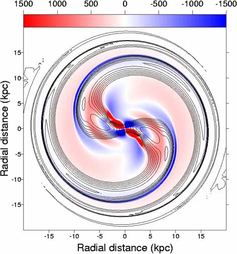
Figure 7: Contour map of the positive stellar density perturbation superimposed onto the map of the mixed velocity dispersion $\sigma^{2}_{r\phi}$. The scale bar is in $({\rm km~{}s}^{-1})^{2}$.

The non-zero $\sigma^{2}_{r\phi}$ indicate that the stellar velocity ellipsoids are not aligned along the local coordinate vector $\hat{r}$ (galactic centre-anticentre direction). The degree of this misalignment is often quantified in terms of a vertex deviation. A classic definition for the vertex deviation is (Binney & Merrifield BM 1998, p. 630)

$$l_{\rm v}={1\over 2}{\rm atan}\left({2\sigma^{2}_{r\phi}\over\sigma^{2}_{rr}-\sigma^{2}_{\phi\phi}}\right).$$ (8)

According to this definition, the vertex deviation takes the values between $-45^{\circ}$ and $+45^{\circ}$. In practice, however, the degree of misalignment of the major axis of stellar velocity ellipsoids with the centre-anticentre direction may exceed these bounds, especially in the regions where the epicycle approximation breaks down. In an extreme case, one might consider a velocity distribution with a vanishing non-diagonal element of $\mathbf{\sigma}$ and $\sigma_{\phi\phi}$ exceeding $\sigma_{rr}$. Then the major principal axis of the velocity ellipsoid will be aligned with the azimuthal direction, yielding $l_{\rm v}=\pi/2$. Therefore, we have extended the classic definition (8) as in VT06

$$\tilde{l}_{\rm v}=\left\{\begin{array}[]{ll}l_{\rm v}&\,\,\mbox{if $\sigma^{2}_{rr}>\sigma^{2}_{\phi\phi}$}\\ l_{\rm v}+{\rm sign}\left(\sigma^{2}_{r\phi}\right)\cdot\displaystyle\frac{\pi}{2}&\,\,\mbox{if $\sigma^{2}_{rr}<\sigma^{2}_{\phi\phi}$},\end{array}\right.$$

According to this re-definition, the vertex deviation can take the values between $-90^{\circ}$ and $+90^{\circ}$. In this paper we extend our previous analysis (VT06) and search for a correlation between the magnitude (and sign) of the vertex deviation and the characteristics of the spiral gravitational field.

Global Fourier amplitudes are often used to quantify the growth rate of spiral perturbations in gravitationally unstable stellar and gaseous discs. These amplitudes are defined as

$$A_{\rm m}(t)={1\over M_{\rm disc}}\left|\int^{r_{\rm out}}_{r_{\rm in}}\int^{2\pi}_{0}\Sigma(r,\phi,t)e^{im\phi}\,r\,dr\,d\phi\right|,$$ (9)

where $m$ is the spiral mode, $M_{\rm disc}$ is the total disc mass, and $r_{\rm in}$ and $r_{\rm out}$ are the disc inner and outer radii, respectively. The global Fourier amplitudes $A(m)$ provide a rough estimate on the total relative amplitude of a spiral density perturbation with mode $m$.

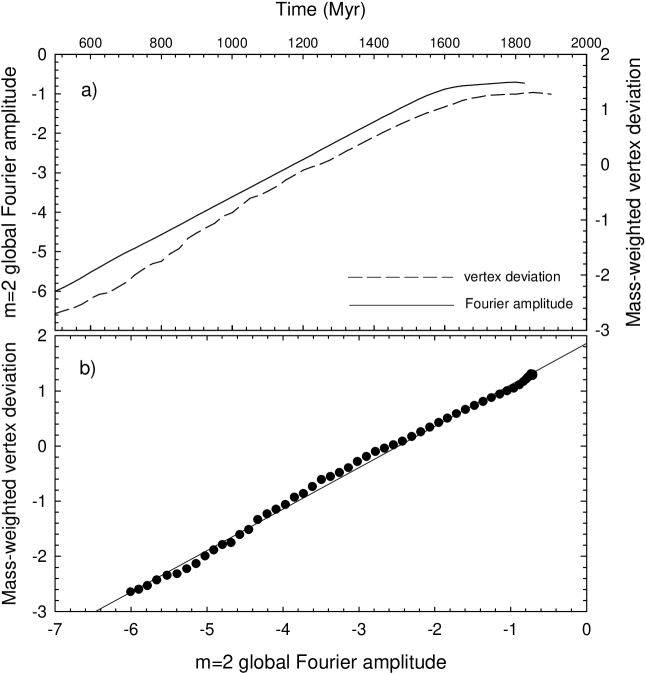
Figure 8: (a) Temporal evolution of the $m=2$ global Fourier amplitude $A_{2}$ (solid line) and mass-weighted vertex deviation $\bar{l}_{\rm v}$ (dashed line) in our model stellar disc. (b) Dependence of $\bar{l}_{\rm v}$ on $A_{2}$ (filled circles). The least-square fit (solid line) yields a near-linear relation $\bar{l}_{\rm v}\propto A_{2}^{0.75}$.

The solid line in Fig. 8a shows the temporal evolution of the dominant $m=2$ global Fourier amplitude (in log units) in our model stellar disc. The $m=2$ amplitude indicates a steady growth of a two-armed spiral structure in the disc from 0.5 Gyr till approximately 1.6 Gyr, when it saturates at $\log A_{2}(t)\approx-0.8$. The subsequent evolution of the stellar disc is characterized by a near-constant value of $A_{2}(t)$ for approximately another 300 Myr, during which the spiral structure is being destroyed by the gravitational torques from spiral arms (this phenomenon is discussed in detail in VT06). It is interesting to see the temporal behaviour of the vertex deviation as the spiral structure grows, saturates, and disperses. The dashed line in Fig. 8a shows the temporal evolution of the mass-weighted vertex deviation (in log units) defined as

$$\bar{l}_{\rm v}=M_{\rm disc}^{-1}\,\sum\limits_{i}dm_{\rm i}\,\tilde{l}_{\rm v,i}\,\,,$$ (10)

where $dm_{\rm i}$ is the stellar mass in the $i$-th computational zone, $\tilde{l}_{\rm v,i}$ is the vertex deviation in the $i$-th zone, and summation is performed over all computational zones. We plot the mass-weighted vertex deviation rather than its arithmetic average to deemphasize high vertex deviations in regions of low stellar density. A correlation between $A_{2}(t)$ and $\bar{l}_{\rm v}$ is clearly evident – both grow and saturate in a similar manner. The saturated value of the mass-weighted vertex deviation is approximately $15^{\circ}$. To emphasize the correlation between $A_{2}$ and $\bar{l}_{\rm v}$, we plot in Fig. 8b the mass-weighted vertex deviation versus the $m=2$ global Fourier amplitude (filled circles), both in log units. The least-square fit shown by the solid lines yields a near-linear relation, $\bar{l}_{\rm v}\propto A_{2}^{0.75}$.

Figure 9: Positive stellar density perturbation superimposed on the vertex deviation map at $t=1.6$ Gyr. Positive and negative vertex deviations are shown with the shadows of red and blue, respectively. The numbers indicate the maximum positive vertex deviation in the inter-arm region and maximum negative vertex deviation in the outer disc. The scale bar is in degrees.

While the mass-weighted vertex deviation appears to correlate globally with the amplitude of spiral density perturbations, it is not clear that this correlation should hold locally as well. Indeed, Fig. 9 shows the vertex deviations in the disc at $t=1.6$ Gyr. The positive and negative vertex deviations are plotted with the shadows of red and blue, respectively. White space corresponds to a near-zero vertex deviation. The black contour lines in Fig. 9 delineate the spiral pattern by showing the regions with a positive relative stellar density perturbation $\zeta(r,\phi)$. The minimum and maximum contour levels correspond to $\zeta=0.1$ and $\zeta=0.8$, respectively. It is clearly seen that the value (and sign) of the vertex deviation does not correlate with the amplitude of the positive stellar density perturbation. In fact, regions with maximum amplitude are characterized by near-zero or small negative vertex deviations ($\tilde{l}_{\rm v}\leq-5^{\circ}$). At the same time, the convex edges of spiral arms, where the stellar density perturbations are small but the gradients of the density perturbations are large, are characterized by quite large negative vertex deviations reaching $\tilde{l}_{\rm v}=-40^{\circ}$ in the outer disc. Considerable positive vertex deviations up to $+30^{\circ}$ are seen between the spiral arms, where the stellar density perturbations are negative. Somewhat surprisingly, the bar has a near-zero vertex deviation but the central regions on both sides of the bar are characterized by the largest vertex deviations up to $\tilde{l}_{\rm v}=\pm 90^{\circ}$. These large values of $\tilde{l}_{\rm v}$ are off the scale in Fig. 9 (and subsequent figures) to emphasize the regions with lower vertex deviations.

6 Discussion

6.1 Comparison with the epicycle approximation

It is often observationally difficult to measure both radial and tangential velocity dispersions of stars. Hence, it is tempting to use equation (5) to derive either of the two dispersions from the known one and the circular speed of stars. One has to keep in mind that equation (5) is valid only in the epicycle approximation, when the epicycle amplitude (deviation from a purely circular orbit) at a specific radial distance $r$ is much less than both $r$ and the scale length for changes in both, the stellar density and dispersion (Kuijken & Tremaine KT 1994, Dehnen dehnen99 1999). The latter condition may become quite stringent, especially near the convex edges of spiral arms. Therefore, it is important to know if equation (5) holds in spiral galaxies with a well-developed spiral structure.

To test the validity of equation (5), we calculate the ratio $\sigma_{\phi\phi}:\sigma_{rr}$ from the model’s known velocity dispersions and compare it with the ratio $(\sigma_{\phi\phi}:\sigma_{rr})_{\rm ep}$ derived using equation (5). From the observational point of view, it is usually difficult to know the exact value of the circular speed $u_{\rm c}$ that enters equation (5), since it requires independent measurements of the axisymmetric gravitational potential in a galaxy. The observers usually apply the local and azimuthally averaged rotation velocities of stars $u_{\phi}$ and $\bar{u}_{\phi}$, respectively, as a proxy for $u_{\rm c}$. The validity of this assumption is checked below.

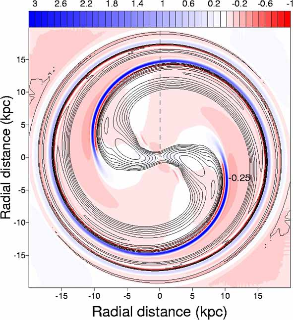
Figure 10: Relative errors between the ratio $(\sigma_{\phi\phi}:\sigma_{rr})$ determined from the model’s known velocity dispersions and ratio $(\sigma_{\phi\phi}:\sigma_{rr})_{\rm ep}$ determined from the epicycle approximation (5) using the local rotational velocity $u_{\phi}$ as a proxy for the circular speed $u_{\rm c}$. The positive and negative relative errors are shown with the shadows of blue and red, respectively. The black contour lines delineate the positive stellar density perturbation at $t=1.6$ Myr.

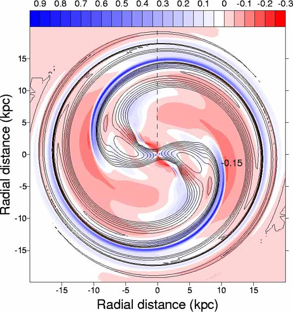
Figure 11: Same as Fig. 10 only with the azimuthally averaged rotational velocity $\bar{u}_{\phi}$ used as a proxy for the circular speed $u_{\rm c}$.

To quantify the deviations from the epicycle approximation in our model spiral galaxy, we calculate the relative errors

$$\xi(r,\phi)={(\sigma_{\phi\phi}:\sigma_{rr})_{\rm ep}-\sigma_{\phi\phi}:\sigma_{rr}\over\sigma_{\phi\phi}:\sigma_{rr}}$$ (11)

using different approximations for the circular speed $u_{\rm c}$. In particular, Fig. 10 and Fig. 11 show the relative errors that are obtained assuming the local rotational velocity $u_{\phi}$ and azimuthally averaged rotational velocity $\bar{u}_{\phi}$ as a substitute for the circular speed $u_{\rm c}$, respectively. The positive and negative errors are plotted with the shadows of blue and red, respectively. The spiral pattern in the disc is outlined by contour lines showing the positive relative stellar density perturbations at $t=1.6$ Gyr.

A visual inspection of Fig. 10 and Fig. 11 indicates that the deviations from the epicycle approximation are largest near the convex edges of spiral arms. To better illustrate this effect, we take a radial cut at $\phi=90^{\circ}$ in Fig. 10 and Fig. 11 (shown by the dashed line) and plot the resulting radial distribution of $\xi(r,\phi=90^{\circ})$ by the solid lines in Fig. 12a and Fig. 12b, respectively. The positive relative stellar density perturbation $\zeta(r,\phi=90^{\circ})$ along the radial cut is shown by the dashed lines. The area below these lines is filled with grey to identify the position of spiral arms. It is evident that if the local rotation velocity of stars $u_{\phi}$ is used as a proxy for the circular speed $u_{\rm c}$ (Figure 12a), then the relative errors can become as large as $\xi=+3.0$ and $\xi=-1.0$ near the outer (convex) edges of spiral arms. If the azimuthally averaged rotational velocity of stars $\bar{u}_{\phi}$ is used as a proxy for $u_{\rm c}$ (Figure 12b), the corresponding relative errors become roughly a factor of three smaller. Yet the relative error can become as large as $\xi=+0.7$ near the outer edge of the innermost spiral at $r\approx 15$ kpc, which renders the epicycle approximation inapplicable in these regions.

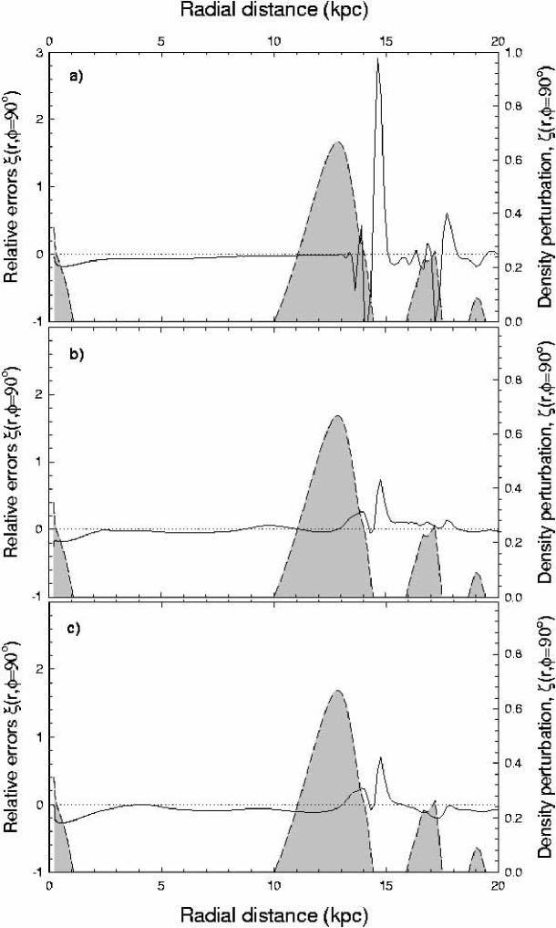
Figure 12: Radial profiles of the relative error $\xi(r,\phi=90^{\circ})$ (solid lines) obtained from (a) Figure 10, (b) Figure 11, and (c) Figure 13 by taking a narrow radial cut at the azimuthal angle $\phi=90^{\circ}$. The positive relative perturbation in the stellar density at $t=1.6$ Gyr is shown by the dashed line.

Finally, we check the validity of the epicycle approximation when the circular speed is determined from the axisymmetric gravitational potential using equation (6) with $\sigma_{rr}$ and $\sigma_{\phi\phi}$ set to zero (cold stellar disc). This approach is accurate but difficult to realize observationally for the reasons explained above. Nevertheless, it might be instructive to compare the ratios of tangential versus radial velocity dispersions obtained in our numerical model with those obtained from the exact epicycle approximation. The corresponding relative errors $\xi(r,\phi)$ are shown in Fig. 13 with the shadows of blue (positive errors) and red (negative errors). The spiral pattern in the disc is outlined by the contour lines showing the positive relative stellar density perturbations at $t=1.6$ Gyr. The convex edges of spiral arms are again characterized by large relative errors. This effect is illustrated in Fig. 12c, which shows $\xi(r,\phi=90^{\circ})$ (solid line) and $\zeta(r,\phi=90^{\circ})$ (dashed line) calculated along the radial cut at $\phi=90^{\circ}$ (Fig. 13, dashed line). The relative errors can become as large as $\xi=+0.7$ near the convex edge of the innermost spiral at $r\approx 15$ kpc and are below $\pm 0.2$ elsewhere.

We conclude that the epicycle approximation is severely in error near the convex edges of spiral arms. On the other hand, the deviation from the epicycle approximation in the inner disc ($r<12$ kpc) remains reasonably small, within $10-20$ per cent. We argue that one should use the azimuthally averaged mean tangential velocity of stars $\bar{u}_{\phi}$ (if available) rather than the local mean tangential velocity $u_{\phi}$ as a proxy for $u_{\rm c}$ and use the epicycle approximation with an extreme caution near the spiral arms. It is interesting to note that the epicycle approximation holds, to within a 20 per cent error, in and near the bar (except for two small spots on both sides of the bar where the relative error can become as large as $\xi=-0.3$).

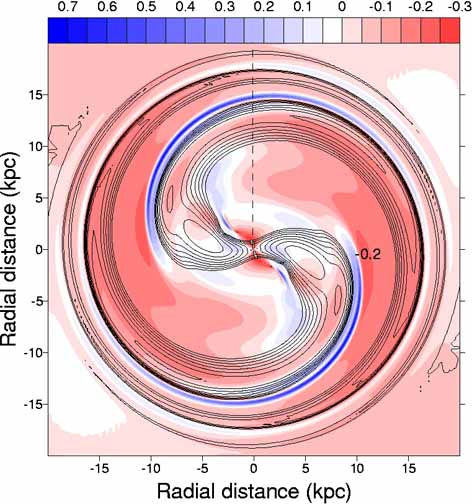
Figure 13: Same as Fig. 10 only with the circular speed determined from equation (6) with the velocity dispersions set to zero.

6.2 Origin of vertex deviation

It is generally thought that two factors contribute to the vertex deviation: (i) moving groups and (ii) a large-scale non-axisymmetric component of the galactic gravitational field (Binney & Merrifield BM 1998). However, it is not clear which of the two factors is more important. The situation may become even more complicated, since the moving groups may partly be caused by the non-axisymmetry in the galactic gravitational field. In order to get a better understanding of the origin of the vertex deviation in our simulation, we analyse the correlation of the vertex deviation with different dynamical quantities.

6.2.1 Correlation of vertex deviation with the gravitational field

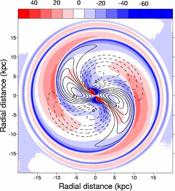
Figure 14: Contour lines showing the relative perturbations in the gravitational potential of the disc superimposed on the spatial distribution of vertex deviations. The positive and negative perturbations are plotted with the solid and dashed lines, respectively. The positive and negative vertex deviations are shown with the shadows of red and blue, respectively. The scale bar is in degrees.

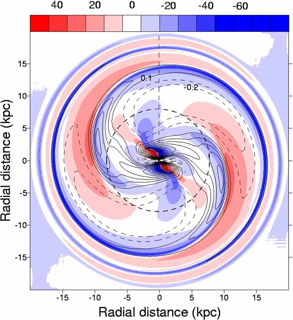
Figure 15: Contour lines showing the relative perturbations in the absolute value of the gravitational potential gradient of the disc superimposed on the spatial distribution of vertex deviations. The positive and negative perturbations are plotted with the solid and dashed lines, respectively. The positive and negative vertex deviations are shown with the shadows of red and blue, respectively. The scale bar is in degrees.

We start by examining the role of the non-axisymmetric gravitational field in generating a vertex deviation. Kuijken & Tremaine (KT 1994) considered non-axisymmetric gravitational potentials typical for a triaxial (ellipsoidal) dark matter halo. They found that the magnitude of the vertex deviation should be proportional to the product of $\sin 2\phi_{\rm b}$ and the ratio of the non-axisymmetric versus axisymmetric contributions to the total gravitational potential $\epsilon_{\Phi}$. Here $\phi_{\rm b}$ is the position angle with respect to the minor axis of the equipotential surfaces of an ellipsoidal halo (see equations [14] and [15] in Kuijken & Tremaine KT 1994). The vertex deviation is expected to be zero near the minor axis of an ellipsoidal halo $(\phi_{\rm b}=0)$. Of course, a direct comparison of our numerical simulations with the analytical predictions of Kuijken & Tremaine is problematic, since the dark matter halo is axisymmetric in our numerical simulations and the non-axisymmetry is introduced by the non-stationary stellar spiral arms and the bar. Moreover, the simulations allow for a completely non-linear evolution, whereas Kuijken & Tremaine’s analysis is based on linear perturbation theory. Nevertheless, it may be helpful to compare two different non-axisymmetric structures and their effect on the spatial distribution of vertex deviations in a stellar disc.

In our model, we calculate the non-axisymmetric gravitational potential by subtracting the gravitational potential of the initial axisymmetric stellar disc $\Phi^{0}_{\rm disc}$ from the current model’s known gravitational potential $\Phi_{\rm disc}$ (which is the sum of contributions from the axisymmetric and non-axisymmetric parts of the stellar disc). The ratio of the non-axisymmetric versus axisymmetric contributions to the total gravitational potential in our model is then determined as

$$\epsilon_{\Phi}={\Phi_{\rm disc}-\Phi^{0}_{\rm disc}\over\Phi^{0}_{\rm disc}}$$ (12)

This quantity calculated at $t=1.6$ Gyr is shown in Fig. 14 by the contour lines. The minimum and maximum contour levels are $\epsilon_{\Phi}=-0.10$ and $\epsilon_{\phi}=+0.12$, respectively, and the step is 0.02. We use dashed and solid lines to differentiate between the negative and positive values of $\epsilon_{\Phi}$, respectively. The positive and negative vertex deviations are shown with the shadows of red and blue, respectively. It is obvious that the magnitude of the vertex deviations in our model stellar disc does not correlate spatially with the ratio of the non-axisymmetric versus axisymmetric stellar gravitational potentials. The maximal vertex deviations (by absolute value) in our model are found along the minor axis of the central bar, whereas in the case of an elliptical halo Kuijken & Tremaine (KT 1994) predicted near-zero vertex deviations there. The reason for this obvious disagreement is not clear and numerical simulations of vertex deviations in models with static elliptical dark matter halos will be presented in a future paper.

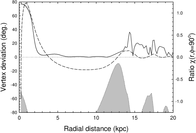
Figure 16: Radial profiles of the vertex deviation by absolute value $|\tilde{l}_{\rm v}|$ (solid line) and relative perturbation in the gravitational potential gradient $\chi$ (dashed line) obtained from Fig. 15 by taking a radial cut along the azimuthal angle $\phi=90^{\circ}$. The dotted line outlines the position of the bar and spiral arms by showing the positive stellar density perturbation. The area below the dotted line is filled with grey.

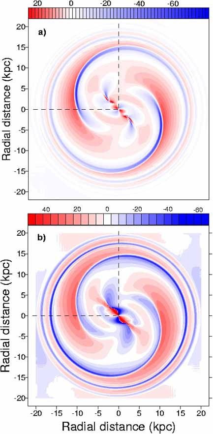
Figure 17: Spatial distribution of (a) derivative $\partial u_{r}/\partial r$ and (b) vertex deviation $\tilde{l}_{\rm v}$ in the stellar disc at t=1.6 Gyr. A clear similarity is seen between the two quantities, especially in the outer parts of the disc. Dashed lines show radial cuts at $\phi=90^{\circ}$ (vertical) and $\phi=180^{\circ}$ (horizontal). Scale bars are in (a) km s^-1 kpc^-1 and (b) in degrees.

However, we should keep in mind that the dynamics of a star is controlled by the gradient of the gravitational potential rather than by the potential itself. We calculate the absolute value of the stellar gravitational potential gradient in the disc as

$$|{\bf\nabla}\Phi_{\rm disc}|=\left[{(\partial\Phi_{\rm disc}/\partial r)^{2}+(r^{-1}\partial\Phi_{\rm disc}/\partial\phi)^{2}}\right]^{0.5}.$$ (13)

This quantity can be regarded as the “strength” of the stellar gravitational field in the disc. We further denote the absolute value of the initial stellar gravitational potential gradient $|{\bf\nabla}\Phi_{\rm disc}|_{0}$ and calculate the relative perturbation in the stellar gravitational potential gradient as

$$\chi(r,\phi)={|{\bf\nabla}\Phi_{\rm disc}|-|{\bf\nabla}\Phi_{\rm disc}|_{0}\over|{\bf\nabla}\Phi_{\rm disc}|_{0}}.$$ (14)

The spatial distribution of $\chi(r,\phi)$ at $t=1.6$ Gyr is shown in Figure 1 with the contour lines. In particular, the solid lines delineate positive relative perturbations in the stellar gravitational potential gradient and dashed lines delineate negative relative perturbations. The minimum and maximum contour levels are $\chi=-0.3$ and $\chi=+1.2$, respectively. The positive and negative vertex deviations $\tilde{l}_{\rm v}$ are shown with the shadows of red and blue, respectively. A visual inspection of Fig. 15 reveals a strong correlation between $l_{\rm v}$ and positive $\chi(r,\phi)$ in the inner disc and a mild correlation between these quantities in the outer disc.

To better illustrate this correlation, we find $\chi$ along a radial cut at $\phi=90^{\circ}$ (dashed line in Fig. 15) and plot the resulting values in Fig. 16 with the dashed line. The corresponding vertex deviation is plotted with the solid line. We should keep in mind that $\tilde{l}_{\rm v}$ changes its sign when the galactic rotation is reversed but $\chi$ does not. Hence, we show the absolute (rather than actual) value of the vertex deviation. The radial position of the spiral arms and the bar at $\phi=90^{\circ}$ is outlined by the dotted line which represents the positive relative perturbation in the stellar surface density (the area below this line is filled with grey). The strongest correlation between $\chi$ and $|\tilde{l}_{\rm v}|$ is seen in the central region where both quantities attain their maximum values. A noticeable correlation between $|\tilde{l}_{\rm v}|$ and $\chi$ is also seen near the outer (convex) edges of spiral arms at $r\approx 14$ kpc and $r\approx 17.5$ kpc. On the other hand, there is little or no correlation in the inter-arm region at $r=(15-16)$ kpc, where $\chi$ is negligible but $|\tilde{l}_{\rm v}|$ can become as large as $20^{\circ}$. A similar lack of correlation is seen at $r=(5-10)$ kpc. We conclude that the relative perturbation in the gravitational potential gradient can only partly account for the magnitude of the vertex deviation in our model disc.

6.2.2 Correlation of vertex deviation with the streaming motions

In this section, we search for the correlation between the vertex deviation and local properties of the stellar velocity field, in particular, the non-circular streaming motions of stars clearly seen in Fig. 2. The streaming motion of stars can be quantified by calculating the spatial derivatives of the radial and tangential mean stellar velocities, namely, $\partial u_{r}/\partial r$, $\partial u_{\phi}/\partial\phi$, and $\partial u_{r}/\partial\phi$. We have examined all three characteristics of the streaming motion and found that $\partial u_{r}/\partial r$ is best suited for our purposes. Figure 17a shows the spatial distribution of $\partial u_{r}/\partial r$ (in units of km s^-1 kpc^-1) in our model stellar disc at $t=1.6$ Gyr. The positive and negative values of this quantity are plotted with the shadows of red and blue, respectively. The spatial distribution of the vertex deviation at $t=1.6$ Gyr, initially shown in Fig. 9, is reproduced in Fig. 17b to facilitate the comparison between $\partial u_{r}/\partial r$ and $\tilde{l}_{\rm v}$. A striking similarity between the spatial distributions of $\partial u_{r}/\partial r$ and $\tilde{l}_{\rm v}$ is clearly seen in the figure, especially in the outer parts of the stellar disc.

To better illustrate the spatial correlation between $\partial u_{r}/\partial r$ and $\tilde{l}_{\rm v}$, we take two radial cuts at $\phi=90^{\circ}$ and $\phi=180^{\circ}$ (shown with dashed lines in Fig. 17) and plot the resulting radial profiles of $\partial u_{r}/\partial r$ (dashed lines) and $\tilde{l}_{\rm v}$ (solid lines) in Fig. 18. Now both quantities happen to have the same sign and the actual values of the vertex deviation are shown. The comparison of Fig. 16 and Fig. 18 demonstrates that the correlation between $\partial u_{r}/\partial r$ and $\tilde{l}_{\rm v}$ is in general better than the correlation between $\chi$ and $\tilde{l}_{\rm v}$. Yet there are regions where $\partial u_{r}/\partial r$ and $\tilde{l}_{\rm v}$ show no correlation. For instance, the derivative $\partial u_{r}/\partial r$ is maximal (by negative value) at approximately 14.5 kpc (Fig. 18a) but the corresponding vertex deviation changes its sign and is characterized by negligibly small values there. Other characteristics of the streaming motion ($\partial u_{\phi}/\partial\phi$ and $\partial u_{r}/\partial\phi$) show similar correlation with the vertex deviation, though less pronounced than in the above case with $\partial u_{r}/\partial r$.

To summarize, the vertex deviation is better correlated with the characteristics of stellar streams such as $\partial u_{r}/\partial r$ than with the relative perturbation in the gravitational potential gradient in the stellar disc. The relative perturbation in the gravitational potential shows essentially no correlation with the vertex deviation, which could be due to the fact that the dynamics of stars is controlled by the gradient of the gravitational potential rather than the gravitational potential itself. It appears that the non-axisymmetric gravitational field of the spiral arms and the bar perturbs stellar orbits by creating large-scale stellar streams. These streams introduce (under specific yet poorly understood conditions) the mixed velocity dispersion $\sigma^{2}_{r\phi}$ into the stellar velocity dispersion tensor and consequently generate the vertex deviation.

This result is in nice qualitative agreement with the linear perturbation analysis in KT91. For instance, their equation (19) shows also a strong correlation between the vertex deviation and the mean velocity field (and its gradients). Moreover, the inner bar region is characterized by rigid rotation, which means KT91’s $\alpha$ becomes unity and the denominator formally vanishes yielding a divergent vertex deviation. Such large vertex deviations are in good agreement with the highest $l_{\rm v}$ values in our simulations found near the central bar.

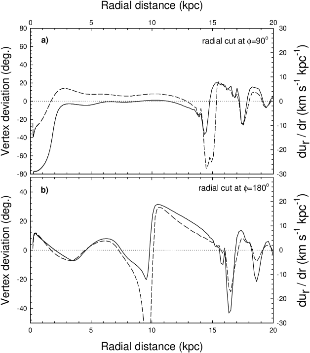
Figure 18: Radial profiles of the vertex deviation (solid lines) and derivative $\partial u_{r}/\partial r$ (dashed lines) obtained from Fig. 17 by taking radial cuts along the azimuthal angles (a) $\phi=90^{\circ}$ and (b) $\phi=180^{\circ}$ at $t=1.6$ Gyr.

6.2.3 Higher-order moments

When applying the Boltzmann moment equations each equation of $n$-th order includes a term of $n+1$-order, by this formally creating an infinite set of equations. In order to end up with a finite set of equations, one has to introduce a closure condition. In hydrodynamics this can be a proper equation of state (e.g. a polytropic equation of state). In stellar hydrodynamics the situation is more complex, because an obvious equation of state does not exist. For instance, an isotropic pressure (or velocity distribution) is guaranteed in a ”normal” gas by collisional relaxation which is usually a rather fast process compared to other timescales like the dynamical timescale. Contrary to a gaseous system, two-body relaxation in a three-dimensional stellar system is a rather slow process. Adopting Spitzer & Hart’s (spitzer71 1971) formula for the relaxation time $\tau_{\rm rel}$,

$$\tau_{\rm rel}=\frac{\sigma^{3}}{15.4G^{2}\rho\,m\ln(0.4N)},$$ (15)

we get with a velocity dispersion $\sigma$ of 10 km s^-1, a typical stellar mass $m$ of 1 M_☉, a local mass density $\rho=0.2~{}\mbox{M${}_{\sun}$}\,\mathrm{pc}^{-3}$ and a number $N$ of stars of $10^{6}$, a relaxation time of about $\tau_{\rm rel}\sim 1.3\cdot 10^{12}\,\mathrm{yr}$. This timescale exceeds the dynamical timescale (and the Hubble time) by far. Even if we adopt the smallest values of about 7 km s^-1 for the velocity dispersions of young stars, the relaxation time is still very long. Thus, in a purely stellar galactic disc two-body relaxation is negligible, and heat conduction terms which are related to the third order moments can be neglected.

In order to check the third order moments quantitatively we started to perform numerical test particle simulations in a given time-dependent disc potential including a spiral. The numerical treatment is similar to the one adopted in Blitz & Spergel (blitz91 1991) and more recently in Minchev & Quillen (minchev07a 2007). First results of these simulations show that the 3rd order terms are small compared to the other moments, by this confirming our numerical treatment. A more detailed analysis of these simulations will be given elsewhere.

7 Summary and Conclusions

In this paper, we present two-dimensional stellar hydrodynamics simulations of a flat galactic disc embedded in a standard dark matter halo, yielding a rigid rotation curve in the central part and a flat rotation curve outside 3 kpc. We solve the Boltzmann moment equations up to second order in the thin-disc approximation and follow the growth of a two-armed spiral structure deeply into the non-linear regime. We analyse in detail the shape and orientation (vertex deviation) of the stellar velocity ellipsoids when the spiral structure has reached a saturation phase. The simulations yield the following main results.

(i) The shape of the stellar velocity ellipsoids (as defined by the ratio $\sigma_{1}:\sigma_{2}$ of the smallest versus largest axes of the stellar velocity ellipsoid) and vertex deviations show large variations over the entire stellar disc. In particular, the radial distribution of the axis ratio $\sigma_{1}:\sigma_{2}$ shows deep minima near the outer (convex) edges of stellar spiral arms.

(ii) The spatial distributions of the radial $\sigma_{rr}$ and tangential $\sigma_{\phi\phi}$ stellar velocity dispersions show a similar two-armed symmetry as the underlying distribution of the stellar surface density.

(iii) The epicycle approximation fails in the regions affected by stellar spiral arms. In particular, it cannot reproduce the tangential-to-radial stellar velocity dispersion ratio $\sigma_{\phi\phi}:\sigma_{rr}$ obtained from the numerical simulations. The deviations from the epicycle approximation are especially large near the outer (convex) edges of stellar spiral arms, where the epicycle approximation may be in error by a factor of two or more.

(iv) Globally, there is an excellent correlation between the mass-weighted vertex deviation (integrated over the whole stellar disc) and the global Fourier amplitude of the stellar density perturbations. However, locally, there is no simple correlation between the vertex deviation and the mass distribution.

(v) The magnitude of the vertex deviation is not correlated with the gravitational potential (mass distribution) and is only weakly correlated with the gradient of the gravitational potential. However, the vertex deviation correlates strongly with the spatial gradients of mean stellar velocities, in particular, with the radial gradient of the mean radial velocity, $\partial u_{r}/\partial r$

(vi) Large-scale, non-circular stellar streams induced by the non-axisymmetric gravitational field of the stellar spiral arms and the bar may be responsible for the failure of the epicycle approximation, large vertex deviations, and peculiar shapes of the stellar velocity ellipsoids.

Our results are in good qualitative agreement with the results of the linear perturbation analysis given in KT91. Moreover, our simulations include also the non-linear stages of the disc evolution when dynamical feedback limits the growth of a spiral structure. The large spatial variations of the properties of the stellar velocity distribution found in our numerical simulations and the mismatch to the epicycle approximation are a caveat for any analysis of observational data which cover larger spatial areas or which include stellar samples coming from a larger spatial region. It will be interesting to check whether features like the ”u-anomaly” could also be created by large-scale streams induced by a transient or swing-amplified spiral.

References

- 1 Alcobé S., Cubarsi R., 2005, A&A, 442, 929
- 2 Athanassoula E., 1984, Phys. Rep., 114, 319
- 3 Bertin G., 2000, Dynamics of Galaxies, Cambridge Univ. Press
- 4 Bienaymé O., 1999, A&A, 341, 86
- 5 Binney J., Merrifield M. S., 1998, Galactic Astronomy, Princeton Univ. Press
- 6 Binney J., Tremaine S., 1987, Galactic Dynamics, Princeton Univ. Press
- 7 Blitz L., Spergel D.N., 1991, ApJ, 370, 205
- 8 Carlberg R.G., Sellwood J.A., 1985, ApJ, 292, 79
- 9 Cuddeford P., Binney J., 1994, MNRAS, 266, 273
- 10 Dehnen W., 1998, AJ, 115, 2384
- 11 Dehnen W., 1999, AJ, 118, 1190
- 12 Dehnen W., 2000, ApJ, 119, 800
- 13 Dehnen W., Binney J.J., 1998, MNRAS, 298, 387
- 14 Mühlbauer G., Dehnen W., 2003, A&A, 401, 975
- 15 De Simone, R., Wu, X., Tremaine, S., 2004 MNRAS, 350, 627
- 16 Eddington A.S., 1906, MNRAS, 67, 34
- 17 ESA, 1997, The Hipparcos and Tycho Catalogues (ESA Sp-1200) (Nordwijk ESA)
- 18 Freeman K.C., 1970, ApJ, 160, 811
- 19 Gerssen J., Kuijken K., Merrifield M.P., 1997, MNRAS, 288, 618
- 20 Goldreich, P, Lynden-Bell, D, 1965, MNRAS, 130, 125
- 21 Hogg D.W., Blanton M.R., Roweis S.T., Johnston K.V., ApJ, 629, 268
- 22 Jenkins, A., Binney, J., 1990, MNRAS, 245, 305
- 23 Julian W.H., Toomre A., 1966, ApJ, 146, 810
- 24 Kapteyn J.C., 1905, Report of the Brit. Ass. for the Advancement of Science, p. 257
- 25 Kaufmann D.E., Contopoulos G., 1996, A&A, 309, 381
- 26 Kerr F.J., Lynden-Bell D., 1985, MNRAS, 221, 1023
- 27 Kobold H., 1890, Astron. Nachr. 125, 65
- 28 Kuijken K., Tremaine S., 1991, in Proc. of Dynamics of Disc Galaxies, Göteborg, B. Sundelius (ed.), p. 71 (KT91)
- 29 Kuijken K., Tremaine S., 1994, ApJ, 421, 178
- 30 Lin, C. C., Yuan, C., Shu, F. H., 1969, ApJ, 155, 721
- 31 Mayor M., 1970, A&A, 6, 60
- 32 Mayor M., 1972, A&A, 18, 97
- 33 Minchev, I., Quillen, A. C., 2006, MNRAS, 368, 623
- 34 Minchev I., Quillen A.C., 2007, MNRAS, 377, 1163
- 35 Minchev I., Nordhaus J., Quillen A.C., 2007, ApJ, 664, L31
- 36 Patsis P., 2006, MNRAS, 369, L56
- 37 Polyachenko V. L., Polyachenko E. V., Strel’nikov A. V., 1997, Astron. Zhurnal, 23, 598 (translated Astron. Lett. 23, 525)
- 38 Ratnatunga K.A., Upgren A.R., 1997, ApJ, 476, 811
- 39 Schwarzschild K., 1907, Nachr. Kgl. Ges. d. Wiss. zu Göttingen, Math. Phys. Klasse, 5, 614
- 40 Spitzer L., Hart M.H., 1971, ApJ, 164, 399
- 41 Toomre, A., 1981, in Fall S. M., Lynden-Bell D., eds, The Structure and Evolution of Normal Galaxies. Cambridge Univ. Press, Cambridge
- 42 Vorobyov E.I., Theis Ch., 2006, MNRAS, 373, 197 (VT06)
- 43 Wielen R., 1974, Highlights of Astronomy, 3, 395
- 44 Wielen R., 1977, A&A, 60, 263
- 45 Yuan C., 1971, AJ, 76, 664