Instabilities of relativistic mean field models and the role of nonlinear terms

Abstract

The instability of nuclear matter due to particle-hole excitation modes has been studied in the frame-work of several relativistic mean field (RMF) models. It is found that both the longitudinal and the transversal modes depend sensitively on the parameter sets used. The important impact of the vector and vector-scalar nonlinear terms on the stability of both modes is demonstrated. Our finding corroborates the result of previous studies, namely that certain RMF models cannot be used in high density applications. However, we show that for certain parameter sets of RMF models this shortcoming can be alleviated by adding these nonlinear terms.

Remarkable progress has been made in constraining the nuclear equation of state (EOS) from astrophysics and heavy ion reactions, i.e., we know at a confident level that the EOS should be soft at moderate densities but relatively stiff at high densities (for recent paper see, e.g., Ref Klahn ). However, the fast development in the unstable nuclear beam facility Mueller will also reveal a lot of unexpected phenomena in unstable nuclei far from the stability line region in the near future. Therefore, a unified model describing simultaneously finite nuclei and matter properties at high densities with high degree of accuracy is not only challenging but also mandatory.

Relativistic mean field (RMF) models have been quite successful in providing a microscopic description of many ground states properties ranging from medium, heavy, up to super-heavy nuclei (for a review see, e.g., Ref PGR1 ). The standard ansatz (S-RMF) uses $\sigma$, $\omega$ and $\rho$ mesons as degrees of freedom with additional cubic and quartic nonlinearities of $\sigma$ meson to describe the interaction. The corresponding parameter sets of this model are known as, e.g., NL-Z Rufa and NL3 Lala . The simplest extension of the S-RMF is achieved by introducing a quartic nonlinearity of the $\omega$ meson in the Lagrangian (V-RMF). The parameter sets TM1 Toki and PK1 Meng belong to this model version. Other extensions (E-RMF) of the S-RMF parameterization are known as G1 and G2 Furnstahl96 . The corresponding model is derived from the effective field theory which allows for possible scalar-vector coupling terms up to fourth order to be present in the Lagrangian. Other interesting properties of the RMF models come from the fact that the relativistic nature of the models and the properties of nuclear matter at saturation are fulfilled while in the extrapolation to higher densities the appearance of acausal behavior (the speed of sound exceeds the speed of light) can be alleviated Jha .

Surprisingly, though, little attention has been given so far to check the matter instability by means of particle-hole excitations with frequency $q_{0}$=0 in the transversal and longitudinal modes, based on these models at high densities. It is understood that this analysis is one of the tools to check the reliability of the models at high densities. Efforts in this direction have been devoted some times ago for the linear model case Horo3 ; Fri , whereas the latest progress can be found in Ref. PGR2 , in which the S-RMF model was used to investigate the instability of symmetric nuclear matter (SNM). The authors of Ref. PGR2 found that the onset of the instability depends sensitively on the parameterization of the model. Parameterizations with a low nucleon effective mass ($m^{*}/m$ $\sim$ 0.5-0.6), which can accurately predict nuclear ground state properties, are critical in the longitudinal mode. The S-RMF model produces also a wide instability regime in the transversal mode, even for the parameterization with high nucleon effective mass or by using a more general functional form of nonlinear $\sigma$-meson self-interactions. In addition, it is known that at the critical density, which is larger than saturation density, the $\sigma$ meson self-interaction in the S-RMF model becomes unstable because the square of the effective $\sigma$ meson mass becomes negative and, as a consequence, an additional instability regime in longitudinal mode appears (see region II in the lower-left panel of Fig. 1). This instability is not present in the linear RMF model. To overcome the mentioned shortcomings, the authors of Ref. PGR2 suggested to add nonlinear terms which contain not only functions of the $\sigma$ meson field, but also of the $\omega$ meson field.

The analysis of the instability in symmetric nuclear matter (SNM) is a first step towards a more comprehensive analysis taking into account matter with multi-component constituents, where the latter plays a key role in our understanding of some stellar matter problems. Due to the simplicity of SNM, many essential physical aspects can be understood lucidly. Therefore, we will revisit the instability problem of the RMF models at high-density SNM but now the role of vector and vector-scalar coupling nonlinearities are taken into account and the effects in the unstable regimes with respect to longitudinal and transversal modes are investigated by using some selected parameterizations of S-RMF, V-RMF and E-RMF models, where the S-RMF is used as the benchmark.

To determine the instabilities of the RMF models, we start from the energy density $\varepsilon$ in SNM which takes the following form,

$$\varepsilon = \varepsilon_{\rm linear}+\frac{1}{3}b_{2}\sigma^{3}+\frac{1}{4}b_{3}\sigma^{4}$$ (1)

$$- \frac{1}{4}d_{1}V_{0}^{4}-d_{2}\sigma V_{0}^{2}-\frac{1}{2}d_{3}\sigma^{2}V_{0}^{2},$$

where for the NL-Z and NL3 parameter sets (S-RMF) the last three terms vanish, and for the TM1 and PK1 parameter sets (V-RMF) only the terms proportional to $d_{2}$ and $d_{3}$ vanish, while for G1 and G2 parameter sets (E-RMF) all parameters are utilized. $\varepsilon_{\rm linear}$ is a function of the kinetic terms of the nucleons, $\sigma$ and $\omega$ masses as well as interactions terms of the nucleons. Using a similar procedure to the one used in Refs. Horo2 ; Horo3 , we can calculate the transversal ($\epsilon_{T}$) and longitudinal ($\epsilon_{L}$) dielectric functions of the RMF models. For SNM, they have simple forms, i.e.,

$$\epsilon_{T} = 1+2d_{V}^{T}\Pi_{T}$$

$$\epsilon_{L} = 1+2d_{S}\Pi_{S}-2d_{V}^{L}\Pi_{V}+4d_{SV}^{L}\Pi_{SV},$$ (2)

with

$$\Pi_{V} \equiv \Pi_{00}-2d_{S}\Pi_{M}^{2}+2d_{S}\Pi_{S}\Pi_{00}$$

$$\Pi_{SV} \equiv \Pi_{M}+2d_{SV}^{L}\Pi_{M}^{2}+2d_{SV}\Pi_{S}\Pi_{00},$$ (3)

where $\Pi_{T}$, $\Pi_{S}$, $\Pi_{00}$, and $\Pi_{M}$ are the transversal, scalar, longitudinal and scalar-vector coupling polarizations of proton or neutron with $q_{0}=0$. In SNM, the values of each polarization for proton and neutron are equal. The explicit forms of these polarizations are given in Refs. Horo2 ; Horo3 . The longitudinal scalar meson propagator is given by

$$d_{S}=\frac{g_{\sigma}}{q^{2}+m^{*~{}2}_{\sigma}+\Delta_{\sigma\omega}{(q^{2}+m^{*~{}2}_{\sigma})}^{-1}},$$ (4)

while the vector meson longitudinal and transversal propagators are

$$d_{V}^{L} = \frac{g_{\omega}}{q^{2}+m^{*~{}2}_{\omega}+\Delta_{\sigma\omega}{(q^{2}+m^{*~{}2}_{\omega})}^{-1}}$$

$$d_{V}^{T} = \frac{g_{\omega}}{q^{2}+m^{*~{}2}_{\omega}},$$ (5)

and the scalar-vector coupling propagator takes the form

$$d_{SV}^{L}=\frac{g_{\omega}g_{\sigma}\Delta_{\sigma\omega}}{(q^{2}+m^{*~{}2}_{\omega})(q^{2}+m^{*~{}2}_{\sigma})+\Delta_{\sigma\omega}},$$ (6)

where $m_{\sigma}^{*~{}2}$= $\partial^{2}\epsilon/{\partial\sigma}^{2}$, $m_{\omega}^{*~{}2}$= $-\partial^{2}\epsilon/{\partial V_{0}}^{2}$ and $\Delta_{\sigma\omega}$=$-\partial^{2}\epsilon/\partial\sigma\partial V_{0}$. It is clear that the NL3, NL-Z, TM1 and PK1 parameterizations have vanishing $\Delta_{\sigma\omega}$ and only S-RMF parameterizations have a constant effective omega-meson mass, which is equal to its bare mass. The unstable regimes are determined from $\epsilon_{L}$, $\epsilon_{T}$ $\leq$ 0. The corresponding results for some selected parameter sets are shown in Fig. 1, where the left panels exhibit the longitudinal modes and the right panels display the transversal ones.

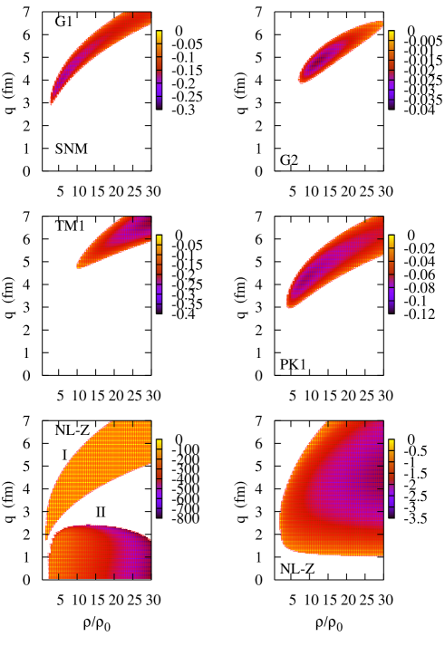
Figure 1: (Color online) Longitudinal (left panels) and transversal (right panels) modes of the instability due to the particle-hole excitation with $q_{0}$ = 0 for the SNM and some selected RMF parameterizations. Different depths of the dielectric functions are shown by different colors (grey scales).

The NL3 and NL-Z models have two instability regimes (I and II). In regime II, NL3 has a deeper $\epsilon_{L}$ valley compared to NL-Z and for each parameter set, the valley in regime II is deeper than regime I. Regime II of the NL-Z parameter set starts to appear at $\rho_{c}$ $\sim$ 2.5 $\rho_{0}$, while for NL3 it starts at $\rho_{c}$ $\sim$ 6.5 $\rho_{0}$, both with $q_{c}$ $\leq$ 2.5 fm. If we use an artificial parameter set with a large nucleon effective mass ($m^{*}/m$ $\geq$ 0.7 at saturation), the unstable regime II disappears. On the other hand, for the V-RMF and E-RMF models with $m^{*}/m$ $\sim$ 0.5-0.6 (the effective nucleon mass range for which the correct spin-orbit splittings is reproduced) at saturation, the regime II does not also exist. For NL-Z, regime I appears quite early, i.e. at $\rho_{c}$ $\sim$ 2.5 $\rho_{0}$ with a relatively small $q_{c}$ ($\sim$ 2 fm), while for NL3 it begins at $\rho_{c}$ $\sim$ 5 $\rho_{0}$ with $q_{c}$ $\sim$ 3 fm.

The vector and vector-scalar coupling in the nonlinear terms of the V-RMF and E-RMF models lead to somewhat narrower unstable regimes compared to the standard one. For TM1, it appears at $\rho_{c}$ $\sim$ 10 $\rho_{0}$ with $q_{c}$ $\sim$ 5 fm, for PK1 it starts at $\rho_{c}$ $\sim$ 5 $\rho_{0}$ with $q_{c}$ $\sim$ 3.5 fm, while for G2 it starts at $\rho_{c}$ $\sim$ 22 $\rho_{0}$ with $q_{c}$ $\sim$ 6.5 fm and for G1 it appears at $\rho_{c}$ $\sim$ 3 $\rho_{0}$ and $q_{c}$ $\sim$ 3 fm. This means that in the V-RMF and E-RMF models there are parameter sets, e.g. TM1 and G2, for which their instabilities in the longitudinal mode can be shifted into the regimes which are physically not too important (large $q_{c}$ and $\rho_{c}$) without losing their accurate predictions in ground-state properties of finite nuclei.

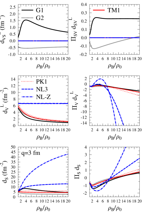
Figure 2: (Color online) Longitudinal scalar ($d_{S}$), vector ($d_{V}^{L}$) and vector-scalar coupling propagators ($d_{VS}^{L}$)(left panels) and the corresponding contributions to the longitudinal dielectric function (right panels). Here $q$ = 3 fm is used.

Contributions of the longitudinal-scalar ($d_{S}$), vector ($d_{V}^{L}$) and vector-scalar ($d_{VS}^{L}$) propagators in the longitudinal dielectric function $\epsilon_{L}$ of Eq. (2) with $q$ = 3 fm (below $q_{c}$ of V-RMF and E-RMF models) for all parameter sets used can be seen in Fig. 2. The density dependence of the $\omega$ meson propagator in the V-RMF or E-RMF models produces a negative vector contribution ($d_{V}^{L}\Pi_{V}$) for all densities. In the case of the G1 parameter set, the vector-scalar coupling ($d_{SV}^{L}\Pi_{SV}$) correction enhances the stability, but this contribution is smaller than G1 albeit with different behavior for G2. Overall, these yield a sufficient suppression to the negative contribution from the scalar one ($d_{S}\Pi_{S}$) at low density regime. As a consequence, a positive $\epsilon_{L}$ is produced. In contrary, for the S-RMF model, a constant $\omega$ meson propagator allows relatively large positive vector and negative scalar contributions. This opens the possibility that $\epsilon_{L}$ becomes negative at low densities.

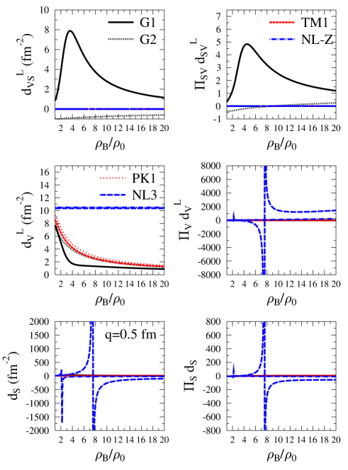
Figure 3: (Color online) Same as Fig. 2 but with $q$ = 0.5 fm. Different with other parameter sets which have small regular contributions, contribution of the NL3 and NL-Z parameter sets at certain density scalar propagator exhibit discontinuities (lower left) which leads to the appearance of the large positive $d_{V}^{L}\Pi_{V}$ (middle right) and negative $d_{S}\Pi_{S}$ (lower right) above this density.

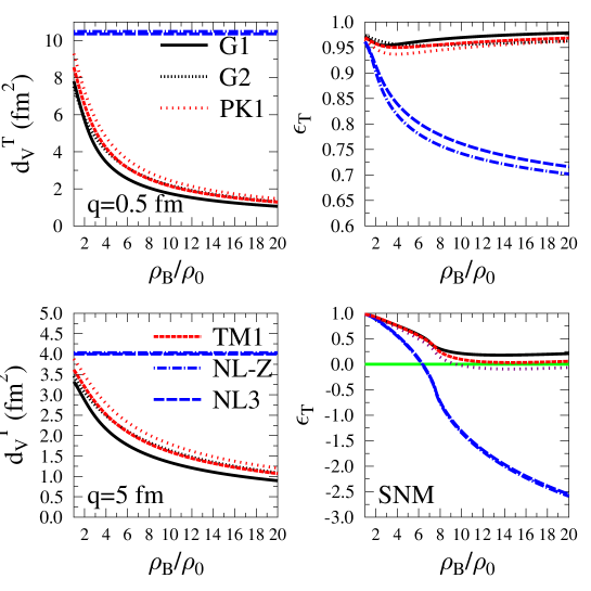
Figure 4: (Color online) Transversal propagators with $q$ = 5 fm (lower-left panel) and $q$ = 0.5 fm (upper-left panel) followed by their transversal dielectric functions (right panels).

The same contributions but with $q$ = 0.5 fm can be seen in Fig. 3. The square effective $\sigma$ meson mass of the NL-Z and NL3 parameter sets becomes negative after reaching a certain critical density ($\rho_{c}$) due to particular parameter values of their scalar nonlinear terms, which leads to the appearance of a discontinuity in $\sigma$ meson propagator at that point. For NL3, the effect is more dramatic but the regime is shifted to a higher critical density compared to the NL-Z parameter set. Furthermore, large positive vector and negative scalar contributions for $\rho$ $\geq$ $\rho_{c}$ appear in this model. Therefore, in this density range, the longitudinal mode becomes unstable, even for very small momentum response ($q\sim$ 0). This is the reason that for both parameter sets the unstable regime II exists.

The S-RMF model has a broad instability for this mode. It does not depend on the parameterization used, except for low momentum response ($q$ $<$ 1 fm). The interesting finding here is that for TM1 and G1 parameter sets the unstable regimes absolutely disappear. The particular parameter values of the vector and vector-scalar nonlinear terms are responsible for this case. While for the PK1 and G2 parameter sets relatively narrow unstable regime are produced, the regimes are also shifted to a relatively high density and large momentum ( $\rho_{c}$ $\sim$ 5 $\rho_{0}$ with $q_{c}$ $\sim$ 3 fm for PK1 and $\rho_{c}$ $\sim$ 8 $\rho_{0}$ with $q_{c}$ $\sim$ 4 fm for G2). This behavior never occurs for the S-RMF model parameterizations. The corresponding results for some selected parameter sets are shown in the right panels of Fig. 1. The role of the density-dependent effective-transversal omega meson propagator of the V-RMF and E-RMF models in stabilizing the transversal modes of the SNM for $q$ $\sim$ 0.5 fm and $q$ $\sim$ 5 fm can be seen in Fig. 4.

If we extend this analysis to the asymmetric nuclear matter (ASM) case (Fig. 5), it is found that different with the unstable regime of transversal mode, the instability of longitudinal mode depends sensitively on the proton fraction in nuclear matter and after a certain critical proton fraction, which is less than the neutron fraction, this unstable regime disappears.

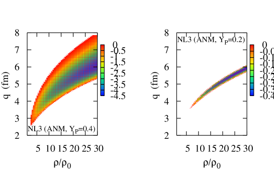
Figure 5: (Color online) Unstable longitudinal regimes I for asymmetric nuclear matter using NL3 parameter set with proton fraction equals 0.4 in the left panel and 0.22 in the right panel.

Thus the longitudinal mode has a strong correlation with the isovector sector of the model. In the case of multi-component matter ($p$, $n$, $e$, and $\mu$) in $\beta$ stability condition, a similar instability trend of the longitudinal and transversal modes with the ones obtained in the SNM case has been met. This means that the nucleons (protons and neutrons) play the main role for determination of the instability. However, a fine tuning in the isovector sector Ant can shift the instability of longitudinal mode to higher critical density and momentum. Details of these results will be reported elsewhere.

In conclusion, we have studied nuclear matter instability caused by particle-hole excitations at $q_{0}$ = 0 in the RMF models at high density for longitudinal and transversal modes. It is found that in both modes the unstable regimes are very sensitive to the parameter set used. This opens the possibility to use the instability analysis as a tool to explore the applicability of parameter sets of the existing RMF models in high density applications. For example, in transversal modes, without the presence of vector and/or vector-scalar nonlinear terms with particular parameter values, the unstable regimes can not vanish. In general additional nonlinear terms in the form of vector and vector-scalar coupling terms of the V-RMF and E-RMF models improve the stability of both models at high densities. Finally we have observed that the longitudinal mode is sensitive to the isovector sector of the model. Thus, some important observables for neutron stars, like proton fraction and asymmetry energy, can be related to this mode.

A.S. would extend his thanks to P-G. Reinhard for useful discussions. A.S. and T.M. acknowledge the support from the Hibah Pascasarjana grant as well as from the Faculty of Mathematics and Sciences, University of Indonesia.

References

- (1) T. Klähn , Phys. Rev. C 74, 035802 (2006).
- (2) A. Mueller, Prog. Part. Nucl. Phys. 46, 359 (2001).
- (3) P.-G. Reinhard, Rep. Prog. Phys 52, 439 (1989).
- (4) M. Rufa, P.-G. Reinhard, J. A. Maruhn, W. Greiner, and M. R. Strayer, Phys. Rev. C 38, 390 (1988).
- (5) G. A. Lalazissis, J. Konig, and P. Ring, Phys. Rev. C 55, 540 (1997).
- (6) Y. Sugahara and H. Toki, Nucl. Phys. A 79, 557 (1994).
- (7) W. Long, J. Meng, N. VanGiai, and S.-G. Zhou, Phys. Rev. C 69, 034319 (2004).
- (8) R. J. Furnstahl, B. D. Serot and H. B. Tang, Nucl. Phys. A 598, 539 (1996); Nucl. Phys. A 615, 441 (1997).
- (9) T. K. Jha, P. K. Raina, P. K. Panda, and S. K. Patra, Phys. Rev. C 74, 055803 (2006).
- (10) K. Lim and C. J. Horowitz, Nucl. Phys. A 501, 729 (1989).
- (11) B. L. Friman and P. A. Henning, Phys. Lett. B 206, 579 (1988).
- (12) H.-G. Doebereiner and P.-G. Reinhard, Phys. Lett. B 227, 305 (1989).
- (13) C. J. Horowitz, and K. Wehberger, Nucl. Phys. A 531, 665 (1991); ibid. Phys. Lett. B 266, 236 (1991).
- (14) A. Sulaksono, P. T. P. Hutauruk, and T. Mart, Phys. Rev. C 72, 065801 (2005).