A Photometric Survey for Variables and Transits in the Field of Praesepe with KELT

Abstract

The Kilodegree Extremely Little Telescope (KELT) project is a small aperture, wide-angle search for planetary transits of solar-type stars. In this paper, we present the results of a commissioning campaign with the KELT telescope to observe the open cluster Praesepe for 34 nights in early 2005. Lightcurves were obtained for 69,337 stars, out of which we identify 58 long period variables and 152 periodic variables. Sixteen of these are previously known as variable, yielding 194 newly discovered variable stars for which we provide properties and lightcurves. We also searched for planetary-like transits, finding four transit candidates. Follow-up observations indicate that two of the candidates are astrophysical false positives, with two candidates remaining as potential planetary transits.

1 Introduction

The field of planet searches has grown tremendously in the past several years. One of the techniques for planet detection that has had recent successes is the search for planets transiting their host stars. Transits of bright stars have great scientific potential, giving clues to the internal structure of planets (Guillot, 2005), their atmospheric composition (Charbonneau et al., 2002), spin-orbit alignment (Gaudi & Winn, 2007), and the presence of rings or moons (Barnes & Fortnoy, 2004) – see Charbonneau et al. (2007) for a comprehensive review.

To date 18 transiting planets are known. Five of them were discovered first through radial-velocity searches and were then found to be transiting, while the rest were discovered by photometric transit surveys. Of those found using the transit method, five were found by the Optical Gravitational Lensing Experiment (OGLE) survey (Udalski et al., 2002a, b, c, 2003, 2004) but have relatively faint ($V>16$) host stars. The eight remaining planets orbit relatively bright ($V\leq 12$) stars and were discovered by small telescopes with wide fields of view (Alonso et al., 2004; Bakos et al., 2007; Burke et al., 2007; Cameron et al., 2007; McCullough et al., 2006; O’Donovan et al., 2006, 2007).

The Kilodegree Extremely Little Telescope (KELT) project is a wide-field, small-aperture survey for planetary transits of stars with $8<V<10$ mag. It is similar to other wide-field transit surveys such as SuperWASP (Pollacco et al., 2006), XO (McCullough et al., 2005), HAT (Bakos et al., 2004), and TrES (Alonso et al., 2004). The justification for the parameters of our survey strategy is described in Pepper, Gould, & DePoy (2003), and the instrumentation, performance, and observing strategy are described in Pepper et al. (2007).

In this paper, we report the results of our commissioning observations. These data were used to establish our operational procedures and to build and test the software pipeline. The purpose was not to discover transits with these observations, but rather to use the data to build the analytical tools for use with comprehensive surveys with KELT. The choice to observe the cluster Praesepe was made based on convenience, as an accessible target at the time of commissioning, and the possibility for scientific potential from studying the variable stars in the cluster. The details of the data set analyzed here are not identical to the main KELT survey data, but we can use the observations to test our ability to obtain transit-quality photometry, defined as lightcurves with low noise, both random and systematic, able to discern astrophysical signals with the timescales and depth of typical planetary transits.

We first briefly review the KELT instrument (§2) and describe the Praesepe observations (§3). We then discuss the data reduction process, (§4), with special attention to the problems that affected the data quality (§4.1), and assess the photometric precision of the data set (§4.6). We explain how we search for variable stars (§5) and transit candidates (§6). We then list the properties of all variable stars detected and display the lightcurves of the periodic variables (§7), and describe the final set of transit candidates and the observations to confirm their nature (§8). We conclude by reviewing the usefulness of this data set and the implications for the full KELT survey (§9).

2 Instrumentation

Here we provide a summary of the full instrumental specifications of KELT that are described in Pepper et al. (2007). The KELT telescope uses an Apogee Instruments AP16E thermoelectrically cooled CCD camera. This camera uses a Kodak KAF-16801E front-side illuminated CCD with $4096\times 4096$ $9\mu$m pixels (36.88 $\times$ 36.88 mm detector area). It has a gain of 3.6 electrons/ADU, readout noise of $\sim$15 e^-, and saturates at 16383 ADU ($\sim$59,000 e^-), with very low dark current. The camera is mounted on a Paramount ME Robotic Telescope Mount manufactured by Software Bisque. The Paramount is a research-grade German Equatorial Mount designed specifically for robotic operation with integrated telescope and camera control. For our observations of Praesepe, we use a Mamiya 645 200 mm f/2.8 APO manual-focus telephoto lens with a 71 mm aperture. This provides a roughly 9$\farcs$5pix^-1 image scale and effective 10$\fdg$8$\times$10$\fdg$8 field of view. A Kodak Wratten #8 red-pass filter with a 50% transmission point at $\sim$490 nm, is mounted in front of the KELT lens. The effective wavelength of the combined Filter+CCD response function (excluding atmospheric effects) is 691nm, with an effective width of 318nm. This results in an effective bandpass that is equivalent to a very broad R-band filter.

The KELT telescope is currently operated at the Irvin M. Winer Memorial Mobile Observatory near Sonoita, Arizona. The site is located at N 31°39′53″, W 110°36′03″, approximately 50 miles southeast of Tucson at an elevation of 1515 meters (4970 feet).

3 Observations

The commissioning campaign targeted a field centered on Praesepe (also called M44 and NGC 2632), an open cluster at a distance of 180 parsecs with an age of $600$ Myr, a metallicity slightly above solar, and little to no reddening (An et al., 2007). Several previous studies have examined the cluster population in efforts to determine the stellar luminosity function and to establish overall cluster membership (Jones & Stauffer, 1991; Adams et al., 2002), in addition to probing the low-mass end of the stellar population (Chappelle et al., 2005). The amount of interstellar extinction, $E(B-V)$, towards the center of Praesepe is 0.029 mag (Schlegel, Finkbeiner, & Davis, 1998), corresponding to $A_{V}=0.09$ for $R_{V}=3.1$.

Our observation were centered on a 10$\fdg$8$\times$10$\fdg$8 field located at J2000 $8^{\rm h}40^{\rm m}06^{\rm s},+19^{\rm o}41^{{}^{\prime}}06^{{}^{\prime\prime}}$, roughly centered on Praesepe. The observing campaign was conducted every clear night from UTC 2005 February 13 until 2005 April 27, obtaining 5220 images during 34 out of the 74 nights of the run. The observations consisted of 60-second observations repeated throughout the night as long as the cluster was above the horizon, resulting in 100 – 200 images each night, with a 90-second cadence. The telescope took images on all nights except those with heavy cloud cover or rain. The quality of our observed nights ranged from completely clear to patchy cloud cover. We rely on several steps of the data reduction process to eliminate images with excessive cloud cover, moonlight, or other problems that compromise photometric quality.

The pointing of the KELT telescope was not perfect, with the coordinates of the field center drifting slowly between images throughout the night. The typical intranight drift was $\sim$25′ ($\sim$160 pixels) in Declination and $\sim$9′ ($\sim$60 pixels) in Right Ascension over the course of many hours. The drift is small compared to the size of the field ($<5$%), but it has two significant effects on our data. First, the drift causes stars at the edges of the field to enter and exit the camera’s field of view during the night, resulting in incomplete lightcurves for those stars. However, since the image quality is poor at the extreme edges of the field, we simply eliminate stars along the field edges from our sample. Secondly, the drift combines with our image reduction software to cause constant stars in certain parts of the field to spuriously appear as variable candidates. See sections §4.2 and §5.2 for details of this effect.

4 Data Reduction

For each of the 5220 images of Praesepe, we subtracted the combined dark for that night, and then divided by a flatfield. Images showing large stellar image FWHM or very high (800 ADU) sky levels are eliminated as “bad”. These sky levels are mostly caused by clouds. In all, 2083 poor-quality images were eliminated from further analysis. The remaining 3137 images were analyzed using the ISIS image subtraction package from Alard & Lupton (1998); Alard (2000). We adopt the implementation of ISIS described by Hartman et al. (2004). We describe that procedure below, and we note where our procedures differ from those of Hartman et al. (2004).

4.1 Changing FWHM

After initial image processing with ISIS, we found that a large number of variable-star candidates had double-valued lightcurves, with the amplitude of many sinusoidal lightcurves being larger on some nights and smaller on others. This variation in amplitude was correlated in time, and appeared to apply mostly to stars in a horizontal zone across the upper part of the chip. We traced the origin of this effect to changing FWHM of the stellar images across our field from night to night. The FWHM does not change significantly horizontally across the field, but it has significant structure in the Y-direction, with the FWHM being large ($\sim 2.8$ pixels) at the top and bottom of the chip, and decreasing linearly towards the middle of the chip in a V-shape, with a minimum FWHM of $\sim 2.0$ pixels at about one third of the distance from the top of the chip.

Had the size and shape of this pattern remained constant throughout the observations, it would not have presented a major problem, since ISIS is able to work with a changing FWHM across the field. However, the vertical-axis position of the FWHM minimum changed significantly between different nights, ranging from the middle of the chip to the top edge. That is, the bottom of the V-shape of the FWHM distribution moved up and down the chip over different nights. The position of the FWHM minimum correlated with the change in amplitude of the lightcurves.

The reason for the double-valued lightcurves relates to the way ISIS works. ISIS requires a reference image that has the smallest FWHM of all images in the set, since it convolves the reference image with the kernel of each of the individual images. With the changing shape of the FWHM pattern in our data, no single image or set of images has a smaller FWHM across the entire field for all the nights. Any given choice for a reference image will contain a horizontal region for which there are other nights where the stars have smaller FWHM values. Regions with smaller PSFs than the reference image on certain nights require deconvolution of the PSFs (i.e. adjusting the stellar images from the reference frame to have smaller PSFs rather than larger). This creates a problem since ISIS works to convolve an image, even with a varying degree across the field, but ISIS is not equipped to correctly deconvolve an image.

We have not been able to absolutely determine the origin of the time-varying FWHM pattern. We believe it could be related to temperature changes from night to night, which affected the 200 mm lens we used for these observations. Since the problem was not detected until after we stopped using the lens, we were unable to test this hypothesis. Instead, our objective is to mitigate the impact of this effect as much as possible and get the best measurements we can out of the data set.

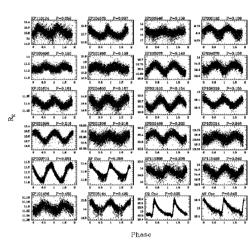
Figure 8: Lightcurves of pulsating periodic variables identified by KELT, sorted by period.

The procedure we adopted is as follows. We first register the images to the same coordinate system, then divide them into four horizontal sections. For each image section we identify a different reference image that has the smallest FWHM out of all images in that section. We then treat the different sections as if they were four separate images, and run each section though the data reduction pipeline with their own reference images to obtain lightcurves (with an additional subdivision step described in §4.2). We also convolve all of the images (but not the reference image) with a Gaussian smoothing function (using a Gaussian with $\sigma=0.6$ pixels) to slightly broaden the PSFs, and thus ensure that the reference image has a smaller FWHM. With this procedure, we are able to eliminate most of the effects of the time-varying FWHM. We are not able to completely eliminate the effect, which can be seen in the slightly double-valued lightcurves of some variables (e.g., see plots of KP300133 and EF Cnc in Figure 8, as well as excessive scatter in the lightcurves of KP113808 and KP118899 in Figure 10).

4.2 Image Subtraction

We perform image subtraction on each section of the 3137 images with ISIS, as described in §4.1. We use a feature of ISIS to further subdivide each section into a grid of subfields, each of which can take on different values for the parameters that are used to convolve the reference image with the kernel for image subtraction. This step is particularly advantageous for large fields of view, in which cloud patterns can be smaller than the size of the field. We subdivide each section into grids from $1\times 5$ to $5\times 5$, depending on the size of the section, and proceed with the image subtraction.

We use DAOPHOT (Stetson, 1987) to identify all of the objects in the field of the reference image of each section, yielding a list of 69,337 stars on all four sections. Stars along the image edges have particularly bad lightcurves, and so we remove all stars within 50 pixels of the edge from further analysis, leaving 66,638 stars for which we generate lightcurves. The ISIS photometry program calculates the flux from a star and its error in each image. In some situations, such as when the star is located at the edge of the chip, or on the edge of one of the of subregions of the subtracted image, the reported flux and error values are not indicative of the true flux. We clean such points from the data by removing data points where the reported flux or error is unphysically high or low. We also remove the two highest and lowest flux measurements from each lightcurve. Removing such a small number of points should not affect detection of variability or transits, but it does help remove spurious points and reduces the number of false positives when searching for variable sources.

4.3 Astrometry and Matching to Known Sources

We use the Astrometrix program to derive astrometric solutions for the reference image, using the Tycho-2 catalog (Høg et al., 2000) to select reference stars. Because of high-order distortions in the corners of the field, we first subdivide the full images into 25 subsections and find separate astrometric solutions for each subimage. The astrometry is good to within an arcsecond, or $\sim 0.1$ pixel.

We match our data set to two catalogs. We first match our stars to the 2MASS catalog (Skrutskie et al., 2006), using a search radius of 9.5 arcseconds or about one KELT pixel. We find that 58,620 out of 66,638 of our KELT stars are in the 2MASS catalog, with 1,559 of them matching to more than one 2MASS source.

We also match our star catalog to known members of the Praesepe cluster. We compiled a catalog from the WebDA website, identifying 832 likely cluster members. After matching to the KELT data using a search radius of 9.5 arcseconds, we find matches to 333 Praesepe member stars. However, many of the stars in the WebDA database are too faint for KELT to detect. If we consider only the 210 WebDA sources with known $V$ magnitudes of $6.8<V<16.4$, we find matches to 147 stars, although the brighter stars are mostly saturated and unusable in the KELT images.

4.4 Photometric Calibration

Our goal for KELT is to obtain highly precise relative photometry, so we do not attempt to achieve extremely precise absolute photometry. The KELT bandpass is an approximate wide $R$ band. We define a KELT magnitude $R_{K}$ to which we calibrate our observations, which is within a few tenths of a magnitude of Johnson $R$ for the bulk of our stars. However, because of our broad filter and wide field, we are susceptible to significant color terms when determining absolute photometry. For stars with a known $(V-I)$ color we can determine the $V$ magnitude to within a tenth of a magnitude. Since we do not know the $(V-I)$ colors of most of our stars, we quote all our observed magnitudes in $R_{K}$, which can be considered to be equivalent to Johnson $R$, modulo a color term which is typically 0.2 magnitudes, but can range from $-0.3$ magnitudes for very blue stars to 0.8 magnitudes for very red stars. See Pepper et al. (2007) for full details about the calibration process.

4.5 Rescaling Errors

One feature of ISIS that has been noted by others is that the formal reported errors tend to be underestimated for brighter stars. Since the errors on individual points are important in the variable selection process, we rescale the errors following the procedure of Kaluzny et al. (1998) and Hartman et al. (2004). We first compute the reduced $\chi^{2}$ for every star

$$\chi^{2}/N_{\rm dof}=\frac{1}{N-1}\sum_{k=1}^{N}\frac{(m_{k}-\mu)^{2}}{\sigma_{k}^{2}},$$ (1)

where the sum is over $N$ observations, $m_{k}$ is the instrumental magnitude with error $\sigma_{k}$, and $\mu$ is the weighted-average instrumental magnitude. We then plot $\chi^{2}/N_{\rm dof}$ versus magnitude and fit a curve to the bottom edge of the heaviest concentration of points. We then multiply the formal errors by the square root of the function of that curve, so that the least variable lightcurves in our data set have $\chi^{2}/N_{\rm dof}$ close to 1 for all magnitudes.

4.6 Photometric Precision

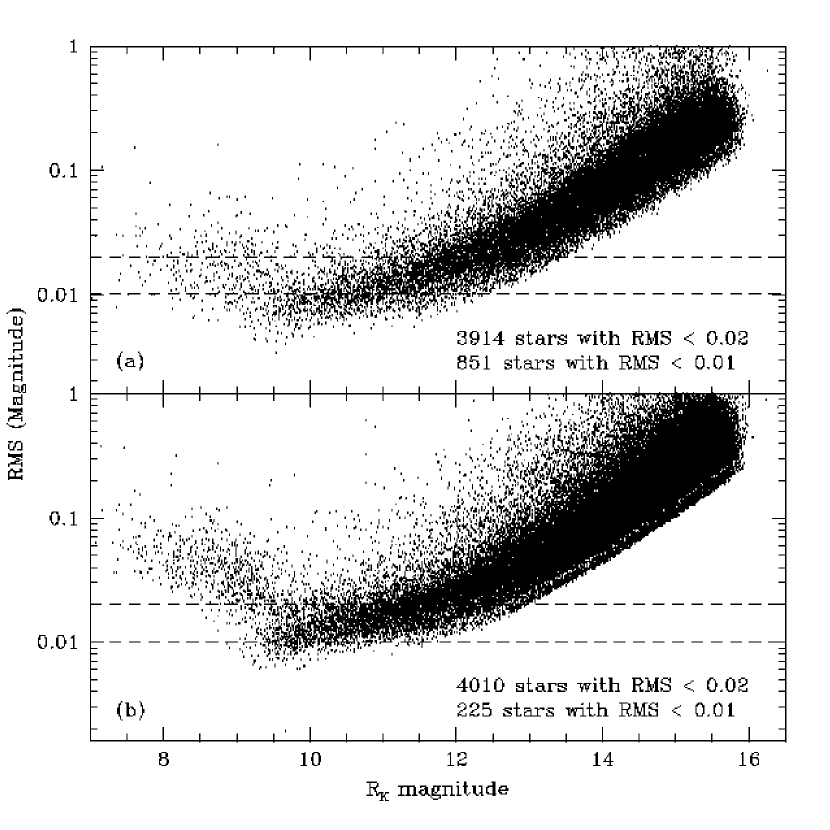
Figure 1: (a) RMS vs. $R_{K}$ magnitude for the 66,638 KELT stars, calculated from 105 observations over the course of one night. (b) RMS plot for the same stars using all 3,137 observations over the full 34 nights. Structure in the plots results from the separate reductions of the four sections of the field to deal with the changes in the FWHM pattern.

A common method for describing the photometric precision of transit searches is to plot the magnitude root-mean-squared (RMS) values of all the lightcurves as a function of magnitude. Because of the FWHM changes described in §4.1, the long term photometric precision has been degraded. However, since the intranight FWHM pattern appears to be stable, we plot the overall RMS and the RMS for one of the nights for all 66,638 stars in Figure 1. Panel (a) of Figure 1 shows the RMS plot for a single night of data, while panel (b) shows the RMS plot for the full 34 nights of data. The dashed horizontal lines show the 2% and 1% RMS limits, which generally define the required sensitivity for detecting Hot Jupiter transits. Two features stand out in these plots. The first is that there are significantly fewer stars with RMS $<1$% in plot (b) than plot (a), although there are about the same number of stars in each plot with RMS $<2\%$. This behavior shows that the inter-night systematics, of which we believe the FWHM changes to be the most significant, become most important at the sub-1% level. The second feature to note is the greater RMS of stars brighter than $R_{K}\approx 9$. The lightcurves of the brightest stars in our sample are dominated by systematic saturation and/or nonlinearity effects that are present during a single night but are more severe over the entire run.

5 Variable Selection

Any transit search will yield a data set suitable for detecting variable stars that are unrelated to transiting planets. We implement several cuts to select promising variable star candidates. We first employ the Stetson $J$ statistic (Stetson, 1996) to find sources that vary coherently in time. We then remove long period variables (LPVs) and run a period-search algorithm to find periodic variables based on the $\sigma_{AoV}$ statistic. We run a periodogram filter to remove spurious variables due to aliasing, resulting in a final set of variable star candidates. Finally, we visually inspect the remaining lightcurves to remove false positives.

5.1 Stetson $J$ Statistic

For each of the 66,638 stars, we compute the Stetson $J$ statistic, using the implementation from Kaluzny et al. (1998). This statistic identifies coherent variable stars by selecting for photometric variations that are correlated in time. After visually examining a number of lightcurves, we define a cutoff of $J=0.7$ to select variable candidates, deliberately choosing a liberal cut on $J$ since we have several more tests to filter out non-variables. We eliminate those stars with $R_{K}<9$, since the lightcurves of the brightest stars in our data set are dominated by systematics due to saturation effects. We also eliminate any star that is less than 10 pixels away from stars with $R_{K}<9$, since extended wings and bleed trails from the bright stars create false variability. We finally remove any candidate that is less than 13 pixels away from a variable candidate with a higher RMS in flux. This eliminates false positives due to constant stars close to true variables. After these cuts we are left with 3430 candidate variable stars.

5.2 Variable Clustering

Among the 3430 variable candidates that pass the cuts described above, most of the stars are clustered around a few of the subsection boundaries, mostly between subsections along the field edges where the fitting parameters vary most, and adjacent subsections closer to the field interior. We assume that all spatial clustering of variables is due to artifacts in the reduction process, and we suspect that the reason for the clustering has to do with how large changes in PSF size and shape across the field affect ISIS.

As described in §3, there was an intranight drift in the telescope pointing. One effect of this drift is that stars undergo slight changes in the PSF shape and size during each night. When ISIS convolves the reference image, it uses different parameters for each subsection (see §4.2). Subsections at the edges of the field experience the strongest optical distortions due to the wide field, and ISIS has the most difficulty fitting the convolution parameters in those areas. At the edges of those subsections the assumptions used to compute the fitting parameters break down. For stars in those areas, the intranight drift means that any consistently inadequate convolution will show up as photometric variability on timescales comparable to the drift rate.

To eliminate false variability due to this effect, we want to remove any candidates that appear in areas with high spatial clustering. However, these areas are not precisely defined – they result from the combination of the ISIS subsection grid, the direction and speed of the drift, and the nature of the optical distortions. We therefore devised an algorithm to remove from our list any stars that are in clustered areas. We divide the entire field into boxes 100 pixels on a side, and count the number of variable candidates in each box. We perform this process four times, with each grid offset from the previous one by 20 pixels in both the X and Y directions. We thus have four staggered grids with which to measure the clustering of the variable candidates. We classify all candidates that appear in a box with more than two other candidates in any of the grids as spurious and eliminate them from our sample, leaving 1101 variable star candidates.

5.3 Identification of Long-Period Variables

There are some stars that pass the cut on $J$ that do not exhibit periodic variability. Many are long-period variables (LPVs) that show monotonically increasing or decreasing brightness during our campaign, some of which may vary periodically but on time scales longer than our campaign. We identify such objects and remove them from our later analysis, which focuses on identifying periodic variables.

To identify LPVs, we use the method described in section 4.3 of Hartman et al. (2004), in which a star is defined as an LPV when a parabola fits the lightcurve much better than a horizontal line. We fit a parabola to the 1,101 remaining variable candidates and calculate the $\chi^{2}/N_{\rm dof}$ for the fit, which we call $\chi^{2}_{N-3}$, along with the $\chi^{2}/N_{\rm dof}$ for the fit to the mean, $\chi^{2}_{N-1}$. There are 52 stars for which $\chi^{2}_{N-3}/\chi^{2}_{N-1}>0.8$, and therefore identified as candidate LPVs, which we eliminate from our remaining variable candidate list. We show the lightcurves of three of our LPVs in Figure 2.

A much smaller fraction of our stars are LPVs (52 out of 66,638 stars, or 0.078%), than the 1,535 LPVs out of 98,000 stars, or 1.6%, found by Hartman et al. (2004). We attribute this difference partly to our greater observational time baseline (74 nights vs. 30 nights), since we end up classifying stars with periodic behavior in that range as regular periodic variables rather than as LPVs. Also, the Praesepe field is located well out of the Galactic Plane, and we therefore expect many fewer background giants than in the field that was observed by Hartman et al. (2004). Since background giants are one of the main types of LPVs (e.g. Mira variables), we would therefore expect fewer LPVs when observing at higher galactic latitudes.

5.4 Periodicity Search

We use the period search algorithm of Schwarzenberg-Czerny (1996) to select periodic variables, adopting the implementation by J. Devor. The Schwarzenberg-Czerny algorithm reports a periodicity likelihood statistic $AoV$, and the Devor method analyzes that information to estimate $\sigma_{AoV}$, a measure of the confidence of the lightcurve’s periodicity. We apply the algorithm to the 1,049 stars remaining in our catalog after removal of the LPVs.

The plot of the best-fit period $P$ vs. $\sigma_{AoV}$ (Figure 3) shows significant aliasing effects at periods that are integer multiples or fractions of 1 day. We thus need to make further cuts to select the true variables from among our list of candidates. First, we construct three histograms in log($P$). Each histogram is shifted in log($P$) by $1/3$ of the width of a bin. All objects that appear in bins in any of the three histograms that have more than seven objects in them are rejected. Any remaining objects with $\sigma_{AoV}>3.3$ are retained. To ensure that true variables were not accidentally eliminated by the binning procedure, any stars that have $\sigma_{AoV}>4.0$ are automatically retained, even if they are caught by the aliasing identification algorithm.

After these cuts, we are left with 182 variable star candidates. We then examine the lightcurves of the remaining candidates by hand, and find that 70 of these are false variables, all of which slightly missed the clustering or alias filters. We also find that six of the candidates, all of which have estimated periods longer than 20 days, are in fact LPVs.

6 Transit Search

The primary goal of the main KELT survey is to identify possible planetary transits. We have used the commissioning data set to build our software pipeline and test our data reduction and analysis procedures, without expecting to identify transit candidates in this data set. However, it is still useful to search for transits, since there is still a chance of discovery, and the transit search could also yield interesting variable stars not found through the earlier variable selection method. Furthermore, we would expect to find false positives in the transit search – astrophysical events that look like transits, such as low-mass stars transiting a solar-type star, which would have lightcurves similar to planetary transits. Finding these events would demonstrate our ability to detect actual transits in the data.

In order to search the data for transits, we take two main steps. The first is to apply a detrending algorithm to reduce or remove a variety of systematics. The second is to run a transit search algorithm over the detrended data and identify transit candidates.

6.1 Detrending

Wide-field transit surveys are susceptible to a number of systematic errors. Observing objects for long stretches of the night requires the telescope to cycle through significant changes in airmass. A wide field of view allows differential cloud patterns to complicate the process of obtaining accurate relative photometry. Temperature changes can affect the optics or detector performance. With so many sources of systematic error, it can be prohibitive to attempt to identify, measure, and compensate for all of these effects. Instead, several methods have been developed to identify all generic systematic effects in data sets of this type. The method we choose to implement is the SYSREM algorithm (Tamuz, Mazeh, & Zucker, 2005; Mazeh, Tamuz, & Zucker, 2007). In brief, this algorithm identifies and subtracts out linear trends that appear in a large portion of lightcurves in a given data set.

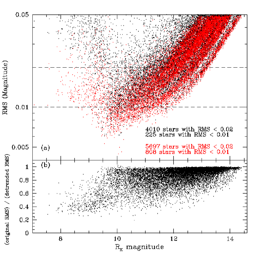
Figure 4: Panel (a) shows the RMS plot for 15,012 stars before (black) and after (red) application of SYSREM detrending. Structure in the locations of the fainter stars results from the separate reductions of the four regions to compensate for the changes in the FWHM pattern. Panel (b) shows the change in RMS by magnitude.

We apply SYSREM to the KELT lightcurves that have been reduced using the procedures described in §4. Since lightcurves with very large variations can create problems for detrending programs, and are not useful for the identification of low level systematics, we only apply SYSREM to the 15,012 stars from our data set with RMS $<5\%$. We recalculate the RMS for the detrended lightcurves and display the results in Figure 4. For most of the lightcurves, detrending improves the RMS by about $\sim 10\%$, although for a few stars, especially towards the bright end, the RMS improves by a factor of 3 to 4.

We suspect that the reason that detrending does not improve the RMS to a greater degree is related the the FWHM problems described in §4.1. Algorithms like SYSREM are designed to remove linear systematics, but it is probable that the systematic errors caused by the FWHM changes are higher order, and so are not rectifiable by linear detrending. Even so, detrending manages to improve the RMS by a small amount, and in some cases works very well, as shown in Figure 5. For the periodic variables we identify with non-detrended RMS below 5%, detrending improves $\sigma_{AoV}$ on average by 10%.

6.2 Transit Selection

To detect transits, we apply a version of the Box-Fitting Least-squares (BLS) transit-search algorithm (Kovacs, Zucker, & Mazeh, 2002) implemented Burke et al. (2006). This algorithm cycles through a range of periods and phases searching for a transit-like event and selects the one with the highest significance. For each lightcurve, we calculate the $\Delta\chi^{2}$ between a constant flux and the best-fit transit model, the $\Delta\chi^{2}_{-}$ for the best-fit antitransit (a brightening rather than dimming), the fraction of $\Delta\chi^{2}$ that results from a single night $f$, and the transit period $P_{t}$. We then examine five parameters: $\Delta\chi^{2}$, $\Delta\chi^{2}/\Delta\chi^{2}_{-}$, $f$, $P_{t}$, and the transit depth. We also examine Digital Sky Survey (DSS) images of the stars which have much higher resolution than KELT, to check whether the single KELT sources consist of blends of more than one star.

Because of the unique characteristics of this data set, we have not elected to construct a rigorous transit selection algorithm using cuts. Instead we sort the lightcurves based on each of the five parameters described above, and examine by eye the 100 best lightcurves identified by each criterion. We classify the lightcurves as either possible transits, variables, or neither. We find four stars with transit-like behavior that are unblended and that are identified with known 2MASS stars. We also find 38 additional variable stars that were not found with the steps described in §5. Of those objects, 31 had $J<0.7$, which is not surprising since the transit-like signals that BLS searches for would not necessarily show the coherent variations characteristic of a variable star with a large $J$ value. Of the seven other stars, one was eliminated by the cluster-rejection routine, and the remaining six had $\sigma_{AoV}<3.3$.

7 Variable Stars

After these procedures we are left with 208 variables, which include the 52 LPVs identified in §5.3, the 6 LPVs found in §5.4, the 112 periodic variables found in §5.4, and the 38 periodic variables found in §6.2.

7.1 Matching to Known Variables

There are 168 known variables within our field of view combining The General Catalog of Variable Stars (GCVS4.2; Samus & Durlevich, 2004) and the New Catalog of Suspected Variable Stars (NSV; Kukarkin et al., 1982),

The magnitudes of the variables are reported in either Johnson $V$ or $U$, or photographic magnitude $p$. The range of magnitudes for which we found variables in the KELT data using all the methods described above are $9<R_{K}<16$. Out of the 168 variables, 72 have reported magnitudes outside that range, and an additional 17 are within $15<V<16$. We only try to match known variables with reported magnitudes between 9 and 15.

We check whether we detect the remaining 79 variables in our data. We search for KELT counterparts using a matching radius of two pixels (19″) and identify 63 matches. Of the 16 known variables we do not detect, three appear either saturated or blended with saturated stars in our data, and 13 do not appear to have counterparts within two pixels of the reported positions, suggesting that the reported positions, proper motions, or magnitudes may be incorrect.

We then compare our list of 208 variables with the 63 detected known variables and find 14 matches. Of the 49 known variables we do not classify as variable through our tests, five have counterparts that are either brighter than $R_{K}=9$ or blended with a bright star. Another 38 are irregular, eruptive, or unspecified variables, which we would not expect to detect with our periodicity-based search algorithms. Three are eclipsing variables of unspecified type with no periods listed in the catalogs. Upon investigation of their KELT counterparts, no eclipses are seen, indicating that either our observations missed the eclipses, or that the eclipse depths were too small to appear in our data. One is listed as an RR Lyrae variable with no period given, for which the KELT lightcurve shows no periodic variation. The remaining two are eclipsing binaries which are removed in the clustering filter, but can be seen in the KELT lightcurves. We add those two stars to our list of variables, giving a total of 210.

We thus have KELT lightcurves for 16 known variables. We find that one KELT LPV is the semi-regular variable GV Cancri. The lightcurve for this object is shown in Figure 2. We find three RR Lyrae variables, CQ Cancri, AN Cancri, and EZ Cancri, the first two of which have periods reported in the catalogs that we confirm. One more variable, EF Cancri, is listed as a W UMa contact eclipsing binary, but the lightcurve, despite the low-quality photometry, appears to indicate that it, too, is an RR Lyrae variable.

We detect six known eclipsing binaries: EH Cancri, GW Cancri, FF Cancri, RU Cancri, NSV 04207, and NSV 04158, in addition to the two eclipsing binaries that were caught by the clustering filter: TX Cancri and RY Cancri. We confirm the reported periods of RY Cancri and TX Cancri, but we find that RU Cancri has a period of 10.0591 days rather than the reported period of 10.172988 days. The remaining variable stars do not have previously reported periods.

The star NSV 04269 is listed as a semiregular variable in the NSV catalog, but our lightcurve shows it to be an eclipsing binary. The star NSV 04069 is not listed as any variable type; we classify it as an eclipsing binary. Lastly, the star FR Cancri is listed as a BY Draconis variable, consistent with our lightcurve.

7.2 Variable Star Catalog

We list the properties of our variable stars in Table 1. For each star we list the KELT ID number, mean $R_{K}$ magnitude, coordinates in Right Ascension and Declination (J2000.0), $JHK$ colors from 2MASS and 2MASS ID for those that matched to 2MASS objects, period (for non-LPVs) in days, type of variable based on our classification, and the GCVS or NSV ID and classification for those that we have identified with previously known variables.

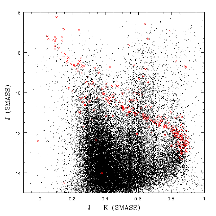
Figure 6: Color-magnitude diagram for cluster stars and field stars. Only field stars that match to a single 2MASS source are plotted; all cluster stars have unique 2MASS matches. Red crosses mark stars listed as members of Praesepe by WebDA.

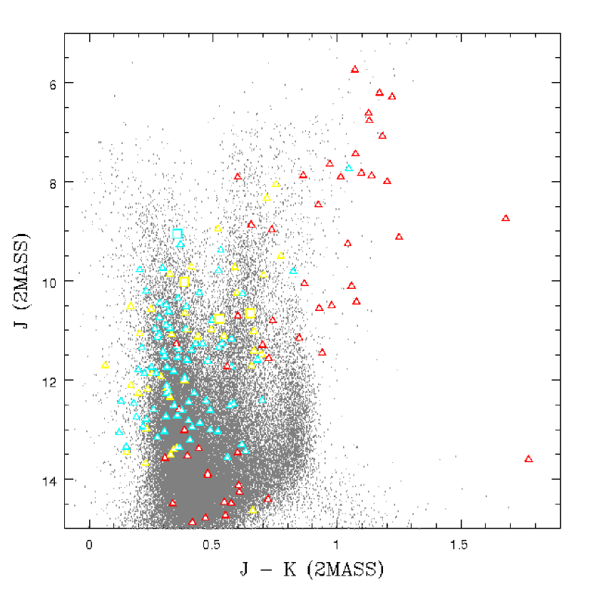
Figure 7: Color-magnitude diagram for variable and non-variable stars. Triangles plot the positions of field variables, while squares plot the four cluster variables. Red symbols mark LPVs, blue symbols mark eclipsing binaries, and yellow symbols mark pulsating variables. Only non-variable stars that match to a single 2MASS source are plotted as dots. The eight variable stars that match to more than one 2MASS source are plotted according to the $J$ and $K$ colors of the nearest 2MASS source. The 27 variables that do not match to any 2MASS source are not plotted.

We plot the 2MASS infrared color-magnitude diagram (CMD) for all our stars in Figures 6 and 7. In Figure 6 we show Praesepe cluster members along with all background stars. The cluster members form a coherent main sequence. The background stars form three populations in $J-K$ color. The largest group, at $J-K\sim 0.4$ consists of main sequence stars. The group at $J-K\sim 0.6$ consists of red giants, and the last group, at $J-K\sim 0.8-0.9$, consists of nearby late-type stars, clearly overlapping the same stellar population at the low end of the Praesepe cluster.

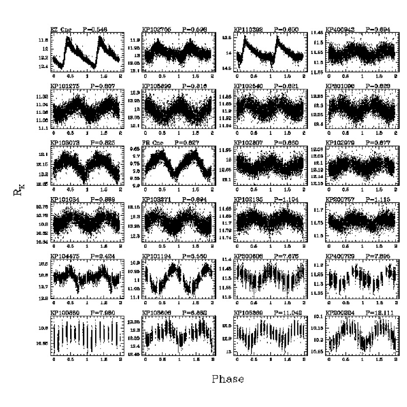
Figure 9: Lightcurves of pulsating periodic variables identified by KELT, sorted by period.

We plot the lightcurves of the periodic variables we identify with the methods described above, along with the two previously known periodic variables that missed our cuts. We classify 48 variable as pulsators, and we plot their lightcurves in Figures 8 and 9. We classify 105 variables as eclipsing binaries, and we plot their light curves in Figures 10 through 14.

8 Transit Candidates

Using the selection process from §6.2, we identify four possible transit candidates. The properties of the four candidates are listed in Table 2, and their lightcurves are shown in Figure 15. These four lightcurves all show events with depths of 5% or less and are not blended with nearby stars in DSS images.

Unfortunately, because of the time that has elapsed between the original observations and the final transit selection, calculations of the eclipse ephemerides for the transit candidates are too inaccurate for targeted photometric follow-up. The periods we derive for the candidates are generally accurate to of order 20 seconds, and since the original observations were taken over two years before the candidates were identified, we do not have ephemerides accurate to within an hour. We therefore use spectroscopic observations to rule out astrophysical false positives.

8.1 Spectroscopic Follow-Up

The four transiting-planet candidates reported in §6.2 were followed up spectroscopically using the CfA Digital Speedometer (Latham, 1992) on the 1.5-m Tillinghast Reflector at the F. L. Whipple Observatory atop Mount Hopkins, Arizona. This instrument has been used extensively for the initial spectroscopic reconnaissance of transiting-planet candidates identified by Vulcan (Latham, 2003) and by TrES and HAT (Latham, 2007). Single-order echelle spectra centered at $5187$ Å  were recorded using an intensified photon-counting Reticon detector with a spectral resolution of 8.5 km s^-1 and typical signal-to-noise ratio of 10 to 20 per resolution element. After rectification to intensity versus wavelength, the observed spectra were correlated against extensive grids of synthetic spectra drawn from a library calculated by Jon Morse using Kurucz (1992) model atmospheres and codes. This allowed us to estimate the effective temperature and surface gravity of the star, assuming solar metallicity, as well as the rotational and radial velocities. For the initial spectroscopic reconnaissance we normally obtain at least two spectra, so that we can look for velocity variations down to the level of about 1 km s^-1 for slowly-rotating solar-type stars.

In the case of KP200924 the first CfA observation revealed that this candidate has a composite spectrum. Plots of the one-dimensional correlation functions clearly show two peaks corresponding to the two stars in a double-lined spectroscopic binary, with a velocity separation of about 200 km s^-1 and rotational broadening of about 65 km s^-1. This must be a grazing eclipsing binary.

For KP102791 we obtained 14 CfA spectra spanning 88 days. The spectroscopic analysis yielded an effective temperature of $T_{\rm eff}=7000$ K, a surface gravity of $\log(g)=4.5$ cm sec^-2, and rotational velocity of $V_{\rm rot}=27.5$ km s^-1. The 14 radial velocities, listed in Table 3, allowed us to derive a single-lined spectroscopic orbit with period $P=3.0227\pm 0.0011$ days, eccentricity $e=0.033\pm 0.026$, orbital semi-amplitude $K=64.9\pm 1.0$ km s^-1, and mass function $f(m)=0.00856\pm 0.00039$ solar masses, see Figure 16. Notice that the spectroscopic period is twice the photometric period, which often happens when the secondary eclipses look similar to the primary eclipses. The eccentricity is indistinguishable from circular, suggesting that the orbit has been circularized by tidal forces. Thus, it is not unreasonable to assume that the rotation of the two stars has been synchronized and aligned with the orbital motion. In this case the observed spectroscopic line broadening can be used to estimate the radius of the primary star, which comes out to about 1.6 solar radii. This in turn implies that the primary has not evolved very much, which is consistent with the surface gravity derived from the spectra. Adopting a mass of 1.5 solar masses for the primary, the mass of the unseen secondary implied by the mass function is about 0.75 solar masses. The ephemeris for future primary eclipses based on just the radial velocity data is $2454170.445\pm 0.069+(3.0227\pm 0.0011)\times E$. Observations with KeplerCam on the 1.2-m reflector at the Whipple Observatory revealed an ingress starting at heliocentric Julian date 2454165.84. Unfortunately the event started six hours later than predicted by the photometric ephemeris available at that time from data that were already two years old, and the ingress was still in progress and already 0.025 magnitudes deep when the telescope reached its pointing limits. It turns out that this particular transit event must have been a secondary eclipse, with its center almost exactly 1.50 cycles after the spectroscopic epoch for primary eclipses quoted above.

For KP102662 we obtained five CfA spectra spanning 33 days. The spectroscopic analysis yielded $T_{\rm eff}=6500$ K, $\log(g)=4.5$ $V_{\rm rot}=3.5$ km s^-1, and mean radial velocity $<V_{\rm rad}>=-20.83\pm 0.37$ km s^-1RMS. The $\chi^{2}$ probability that the observed velocity residuals are consistent with Gaussian errors and constant velocity is $P(\chi^{2})=0.82$, so if the transit-like lightcurve observed for the visible star in this system is caused by an orbiting companion, the companion mass must be less than just a few Jupiter masses. On this basis KP102662 survives as a viable transiting planet candidate. However, the transit lightcurve looks V-shaped and rather too deep to allow a Jupiter-sized planet. Nevertheless, this candidate deserves further follow-up observations. Obtaining a high-quality lightcurve would probably prove to be time consuming, because the ephemeris is based on data that are already two years old, so highly precise radial velocities may be the best way to proceed.

For KP103126 we obtained six CfA spectra spanning 58 days. The spectroscopic analysis yielded $T_{\rm eff}=6250$ K, $\log(g)=4.5$ cm sec^-2, $V_{\rm rot}=0.5$ km s^-1, $<V_{\rm rad}>=-11.49\pm 0.79$ km s^-1RMS, and $P(\chi^{2})=0.035$. The velocity residuals are a bit larger than expected, but still consistent with an orbiting companion that is no more than several Jupiter masses. Thus this candidate also survives as a viable transiting-planet candidate, one that might reward highly precise radial-velocity observations.

9 Conclusions

This paper has presented an analysis of the KELT commissioning data, consisting of a 74-day campaign towards the Praesepe open cluster. We obtained lightcurves for over 66,000 stars, and identified 210 variable stars, of which 194 were not previously known as variable.

We have also searched for planetary transits, finding four transit candidates. Follow-up observations have ruled out two of the candidates as being non-planetary in origin, while two remain as possible planetary systems. This data set has served as the testbed for developing the variable and transit search algorithms that will be used to analyze data from the main KELT survey, and has demonstrated the ability of KELT to detect signals at the level of precision of transiting planets.

Table 1: Variable Stars Identified in KELT Observations of Praesepe

KELT	$R_{K}$	RA	Dec	$J$	$H$	$K$	2MASS	Period	KELT	GCVS/NSV	GCVS/NSV
ID #		(J2000.0)	(J2000.0)				ID #	(days)	Class.	ID	Class.
KP100169	9.136	133.01755	14.58464	6.212	5.349	5.041	J08520421+1435047	$\cdots$	LPV	$\cdots$	$\cdots$
KP100282	9.495	131.11816	20.20117	9.291	8.881	8.832	J08442835+2012042	1.2065	EB	$\cdots$	$\cdots$
KP100305	9.605	133.03393	21.84911	7.440	6.605	6.366	J08520814+2150567	$\cdots$	LPV	$\cdots$	$\cdots$
KP100306	9.606	131.14550	16.28497	7.646	6.826	6.675	J08443491+1617058	$\cdots$	LPV	$\cdots$	$\cdots$
KP100336	9.686	132.50840	17.87422	9.368	8.983	8.838	J08500201+1752271	5.2301	EB	$\cdots$	$\cdots$
KP100445	9.930	130.00713	18.99986	9.053	8.767	8.698	J08400171+1859594	0.3828	EB	TX Cnc	W UMa
KP100561	10.149	130.99077	16.71554	7.741	6.932	6.694	J08435778+1642559	1.0438	EB	$\cdots$	$\cdots$
KP100626	10.274	135.20934	18.27620	6.291	5.470	5.069	J09005024+1816343	$\cdots$	LPV	$\cdots$	$\cdots$
KP100722	10.408	131.77529	21.03571	8.869	8.321	8.215	J08470606+2102085	$\cdots$	LPV	$\cdots$	$\cdots$
KP100880	10.625	135.54936	16.38090	9.720	9.387	9.308	J09021184+1622512	7.9795	Puls	$\cdots$	$\cdots$
KP100886	10.630	131.78774	23.84970	$\cdots$	$\cdots$	$\cdots$	$\cdots$	$\cdots$	LPV	$\cdots$	$\cdots$
KP100920	10.671	131.08151	20.80536	9.907	9.638	9.643	J08441956+2048192	0.4106	EB	$\cdots$	$\cdots$
KP101034	10.796	130.48279	19.68971	9.869	9.627	9.544	J08415586+1941229	0.8894	Puls	$\cdots$	$\cdots$
KP101095	10.871	133.01889	15.36116	10.206	10.011	9.977	J08520453+1521401	0.4240	EB	$\cdots$	$\cdots$
KP101194	10.969	134.29383	17.97599	9.730	9.240	9.143	J08571051+1758335	3.5604	Puls	$\cdots$	$\cdots$
KP101231	11.000	134.29044	18.94559	9.794	9.391	9.272	J08570970+1856441	0.2910	EB	$\cdots$	$\cdots$
KP101257	11.028	133.13490	16.80922	11.327	11.044	10.973	J08523237+1648331	3.5740	EB	$\cdots$	$\cdots$
KP101275	11.053	130.47658	19.25742	10.026	9.732	9.643	J08415437+1915267	0.8067	Puls	$\cdots$	$\cdots$
KP101456	11.209	133.22672	21.98288	10.572	10.414	10.322	J08525441+2158583	0.4351	Puls	$\cdots$	$\cdots$
KP101496	11.253	133.20090	18.39749	9.254	8.428	8.211	J08524821+1823509	$\cdots$	LPV	$\cdots$	$\cdots$
KP101511	11.263	129.92462	14.08659	10.405	10.021	9.990	J08394194+1405136	3.3393	EB	$\cdots$	$\cdots$
KP101549	11.289	132.56274	23.22313	$\cdots$	$\cdots$	$\cdots$	$\cdots$	$\cdots$	LPV	$\cdots$	$\cdots$
KP101674	11.402	132.54651	23.61266	$\cdots$	$\cdots$	$\cdots$	$\cdots$	0.1612	Puls	$\cdots$	$\cdots$
KP101756	11.464	130.16648	23.26186	$\cdots$	$\cdots$	$\cdots$	$\cdots$	0.2958	Puls	EF Cnc	W UMa
KP101831	11.509	131.82932	20.83213	10.481	9.999	9.859	J08471903+2049556	$\cdots$	LPV	$\cdots$	$\cdots$
KP101896	11.552	132.52862	23.52362	$\cdots$	$\cdots$	$\cdots$	$\cdots$	$\cdots$	LPV	$\cdots$	$\cdots$
KP101921	11.573	132.90697	20.04515	10.261	9.730	9.642	J08513767+2002425	0.5766	EB	$\cdots$	$\cdots$
KP102135	11.692	133.33712	22.75218	10.656	10.317	10.270	J08532090+2245078	1.1039	Puls	$\cdots$	$\cdots$
KP102245	11.749	132.76992	21.70140	10.895	10.622	10.585	J08510478+2142050	0.5188	EB	$\cdots$	$\cdots$
KP102395	11.819	134.66732	17.24139	10.707	10.209	10.107	J08584015+1714290	$\cdots$	LPV	$\cdots$	$\cdots$
KP102511	11.878	131.20885	20.18795	9.815	9.174	8.992	J08445012+2011166	0.5584	EB	$\cdots$	$\cdots$
KP102540	11.894	130.44375	14.87345	10.991	10.713	10.598	J08414649+1452244	0.8213	Puls	$\cdots$	$\cdots$
KP102588	11.916	132.71335	19.35729	11.746	11.554	11.495	J08505120+1921262	1.3244	EB	NSV 04269	V
KP102705	11.980	134.51968	22.63479	11.082	10.806	10.749	J08580472+2238052	0.5978	Puls	$\cdots$	$\cdots$
KP102807	12.030	132.66099	16.71456	10.993	10.610	10.500	J08503863+1642524	0.8599	Puls	$\cdots$	$\cdots$
KP102811	12.034	133.42089	22.34420	10.791	10.374	10.295	J08534101+2220391	0.6102	EB	$\cdots$	$\cdots$
KP102836	12.047	134.25911	23.52545	$\cdots$	$\cdots$	$\cdots$	$\cdots$	3.1742	EB	$\cdots$	$\cdots$
KP102908	12.082	134.96979	17.47890	10.108	9.268	9.050	J08595274+1728440	$\cdots$	LPV	$\cdots$	$\cdots$
KP102979	12.112	130.63708	21.17889	11.707	11.658	11.643	J08423289+2110440	0.8773	Puls	$\cdots$	$\cdots$
KP103010	12.124	130.34124	18.13422	11.430	11.184	11.132	J08412189+1808031	1.2578	EB	$\cdots$	$\cdots$
KP103073	12.150	130.02381	19.02520	10.658	10.149	10.009	J08400571+1901307	0.8246	Puls	$\cdots$	$\cdots$
KP103143	12.176	132.41259	23.80157	$\cdots$	$\cdots$	$\cdots$	$\cdots$	1.2542	EB	$\cdots$	$\cdots$
KP103254	12.226	133.24489	23.78463	$\cdots$	$\cdots$	$\cdots$	$\cdots$	0.5458	Puls	EZ Cnc	RR Lyr
KP103267	12.229	133.18612	22.51454	10.059	9.452	9.219	J08524466+2230523	$\cdots$	LPV	$\cdots$	$\cdots$
KP103271	12.232	131.87079	16.27255	11.116	10.659	10.573	J08472898+1616211	0.8943	Puls	$\cdots$	$\cdots$
KP103285	12.237	131.47646	19.58272	11.378	11.071	11.016	J08455435+1934577	0.3550	EB	$\cdots$	$\cdots$
KP103393	12.280	132.90310	20.05444	11.801	11.626	11.603	J08513674+2003159	0.5763	EB	$\cdots$	$\cdots$
KP103585	12.345	131.02744	18.51100	11.539	11.213	11.182	J08440658+1830395	4.4082	EB	$\cdots$	$\cdots$
KP103593	12.348	134.67894	14.88607	11.406	11.075	10.993	J08584294+1453098	0.3536	EB	$\cdots$	$\cdots$
KP103608	12.353	130.90608	19.93658	11.018	10.508	10.354	J08433745+1956116	8.8821	Puls	$\cdots$	$\cdots$
KP103772	12.410	130.51883	24.10952	$\cdots$	$\cdots$	$\cdots$	$\cdots$	0.2603	EB	$\cdots$	$\cdots$
KP104115	12.530	134.02845	14.64294	11.822	11.520	11.481	J08560682+1438345	2.6984	EB	$\cdots$	$\cdots$
KP104166	12.549	130.52602	21.26102	10.554	9.810	9.626	J08420624+2115396	$\cdots$	LPV	$\cdots$	$\cdots$
KP104174	12.552	130.67742	21.41570	11.518	11.259	11.213	J08424258+2124565	0.3637	EB	NSV 04207	V
KP104185	12.557	132.05289	21.12052	11.272	10.940	10.843	J08481269+2107138	0.2814	EB	GW Cnc	W UMa
KP104317	12.599	130.33974	19.00734	11.592	11.293	11.198	J08412153+1900264	0.3464	EB	$\cdots$	$\cdots$
KP104332	12.602	135.08220	14.35794	11.736	11.271	11.162	J09001972+1421285	0.2698	EB	$\cdots$	$\cdots$
KP104424	12.629	131.62549	22.65176	10.807	10.190	10.067	J08463011+2239063	$\cdots$	LPV	$\cdots$	$\cdots$
KP104475	12.644	132.03164	23.12175	$\cdots$	$\cdots$	$\cdots$	$\cdots$	2.4236	Puls	$\cdots$	$\cdots$
KP104572	12.670	130.57458	16.39318	12.266	12.065	12.067	J08421789+1623354	0.0865	Puls	$\cdots$	$\cdots$
KP104597	12.676	130.52484	21.43683	11.868	11.697	11.646	J08420596+2126125	0.4586	EB	$\cdots$	$\cdots$
KP104630	12.683	134.71800	21.07624	10.058	9.433	9.190	J08585231+2104344	$\cdots$	LPV	$\cdots$	$\cdots$
KP104850	12.741	132.90945	16.52710	10.424	9.556	9.346	J08513826+1631375	$\cdots$	LPV	$\cdots$	$\cdots$
KP104855	12.742	129.97762	19.82194	12.514	12.217	12.171	J08395462+1949189	1.0929	EB	RY Cnc	EA/SD
KP104917	12.760	131.04394	22.25307	11.804	11.071	10.945	J08441054+2215110	0.7091	EB	$\cdots$	$\cdots$
KP105076	12.804	130.07613	16.60935	12.014	11.700	11.632	J08401827+1636336	0.1489	Puls	$\cdots$	$\cdots$
KP105119	12.815	130.94612	14.90738	12.433	12.299	12.305	J08434706+1454265	0.7477	EB	$\cdots$	$\cdots$
KP105369	12.877	130.41766	14.80151	11.489	10.980	10.794	J08414023+1448054	11.0424	Puls	$\cdots$	$\cdots$
KP105756	12.971	135.26383	17.89894	11.273	11.051	10.922	J09010331+1753561	$\cdots$	LPV	$\cdots$	$\cdots$
KP105772	12.975	131.03903	17.06938	11.729	11.250	11.172	J08440936+1704097	$\cdots$	LPV	$\cdots$	$\cdots$
KP105793	12.979	132.74935	13.96247	12.230	11.954	11.909	J08505984+1357448	0.3216	EB	$\cdots$	$\cdots$
KP105899	13.005	133.45578	20.85212	11.412	10.845	10.747	J08534938+2051076	0.8162	Puls	$\cdots$	$\cdots$
KP106106	13.054	135.21007	23.62369	$\cdots$	$\cdots$	$\cdots$	$\cdots$	0.6997	EB	$\cdots$	$\cdots$
KP106218	13.077	133.14519	22.48431	11.156	10.453	10.309	J08523484+2229035	$\cdots$	LPV	$\cdots$	$\cdots$
KP106227	13.080	133.37819	14.13207	11.563	11.003	10.839	J08533076+1407554	$\cdots$	LPV	$\cdots$	$\cdots$
KP106319	13.096	130.44779	21.97142	12.161	11.909	11.847	J08414746+2158171	0.1846	Puls	$\cdots$	$\cdots$
KP106351	13.102	134.54297	15.80525	12.112	11.941	11.944	J08581031+1548188	0.5430	Puls	AN Cnc	RR Lyr
KP106452	13.122	131.34256	15.27477	12.187	11.994	11.951	J08452221+1516291	0.5246	Puls	CQ Cnc	RR Lyr
KP106608	13.157	133.67184	19.11521	12.352	12.038	11.998	J08544124+1906547	0.3396	EB	$\cdots$	$\cdots$
KP106885	13.213	133.82978	16.43977	11.455	10.694	10.515	J08551914+1626231	$\cdots$	LPV	$\cdots$	$\cdots$
KP107014	13.234	130.22716	14.42231	12.345	12.011	12.019	J08405451+1425203	0.2465	Puls	$\cdots$	$\cdots$
KP107531	13.333	129.98160	23.33538	$\cdots$	$\cdots$	$\cdots$	$\cdots$	0.5516	EB	$\cdots$	$\cdots$
KP107924	13.408	135.19565	15.42220	12.941	12.796	12.724	J09004695+1525199	0.5268	EB	$\cdots$	$\cdots$
KP108285	13.473	130.92216	18.42757	12.735	12.477	12.425	J08434131+1825392	0.3360	EB	$\cdots$	$\cdots$
KP108858	13.569	130.25118	13.67656	12.607	12.213	12.119	J08410028+1340356	0.2986	EB	$\cdots$	$\cdots$
KP109198	13.619	133.45391	21.49120	13.066	12.953	12.946	J08534893+2129283	1.7433	EB	$\cdots$	$\cdots$
KP109247	13.625	133.88598	14.54473	13.160	12.925	12.885	J08553263+1432410	0.4205	EB	$\cdots$	$\cdots$
KP110021	13.734	132.80862	16.07745	13.036	12.801	12.732	J08511406+1604388	0.3860	EB	$\cdots$	$\cdots$
KP110124	13.751	134.72799	15.36940	13.450	13.295	13.300	J08585471+1522098	0.0576	Puls	$\cdots$	$\cdots$
KP110177	13.760	130.17535	14.98393	12.410	11.867	11.713	J08404208+1459021	0.4420	EB	$\cdots$	$\cdots$
KP110305	13.777	130.52273	22.41861	12.483	12.007	11.900	J08420545+2225069	0.2719	EB	$\cdots$	$\cdots$
KP110392	13.792	130.19981	15.41455	13.402	13.115	13.061	J08404795+1524523	0.6004	Puls	$\cdots$	$\cdots$
KP110617	13.826	131.51008	15.44463	$\cdots$	$\cdots$	$\cdots$	$\cdots$	0.3395	EB	$\cdots$	$\cdots$
KP110674	13.837	133.33587	23.52222	$\cdots$	$\cdots$	$\cdots$	$\cdots$	11.0384	EB	$\cdots$	$\cdots$
KP110871	13.864	130.70418	15.39379	12.524	12.010	11.957	J08424900+1523376	0.2836	EB	$\cdots$	$\cdots$
KP110876	13.865	131.03416	16.84885	12.866	12.492	12.420	J08440819+1650558	0.3013	EB	$\cdots$	$\cdots$
KP111363	13.933	134.00672	18.27980	$\cdots$	$\cdots$	$\cdots$	$\cdots$	$\cdots$	LPV	$\cdots$	$\cdots$
KP112203	14.042	132.87884	21.75790	13.009	12.588	12.521	J08513092+2145284	0.3567	EB	$\cdots$	$\cdots$
KP112538	14.086	129.95615	15.42027	13.304	12.770	12.688	J08394947+1525129	0.2722	EB	$\cdots$	$\cdots$
KP113453	14.197	132.70565	16.31045	13.683	13.550	13.455	J08504935+1618376	0.3395	Puls	$\cdots$	$\cdots$
KP113808	14.236	131.51525	20.96654	13.211	12.920	12.805	J08460366+2057595	0.3182	EB	$\cdots$	$\cdots$
KP114383	14.301	131.15271	21.75311	13.371	13.095	13.007	J08443665+2145111	0.3478	EB	$\cdots$	$\cdots$
KP114757	14.344	133.70368	20.10852	13.602	12.676	11.830	J08544888+2006306	$\cdots$	LPV	$\cdots$	$\cdots$
KP115386	14.408	134.78593	23.89257	$\cdots$	$\cdots$	$\cdots$	$\cdots$	0.2981	Puls	$\cdots$	$\cdots$
KP115639	14.434	131.93564	23.76530	$\cdots$	$\cdots$	$\cdots$	$\cdots$	0.5692	EB	$\cdots$	$\cdots$
KP115973	14.469	135.41519	16.40212	13.531	13.232	13.135	J09013964+1624076	$\cdots$	LPV	$\cdots$	$\cdots$
KP118312	14.698	132.30275	20.90523	13.923	13.617	13.445	J08491266+2054188	$\cdots$	LPV	$\cdots$	$\cdots$
KP118899	14.754	134.88939	21.16955	13.444	12.955	12.812	J08593345+2110103	0.2897	EB	$\cdots$	$\cdots$
KP119499	14.808	135.31678	19.63988	13.468	12.922	12.869	J09011602+1938235	$\cdots$	LPV	$\cdots$	$\cdots$
KP121436	14.975	130.64868	20.64923	13.881	13.436	13.403	J08423568+2038572	$\cdots$	LPV	$\cdots$	$\cdots$
KP126266	15.351	132.71161	19.68410	14.129	13.679	13.526	J08505078+1941027	$\cdots$	LPV	$\cdots$	$\cdots$
KP127604	15.455	131.49181	19.93790	14.733	14.361	14.183	J08455803+1956164	$\cdots$	LPV	$\cdots$	$\cdots$
KP127745	15.466	132.14931	20.92373	14.871	14.607	14.455	J08483583+2055254	$\cdots$	LPV	$\cdots$	$\cdots$
KP128381	15.511	132.94836	16.20497	14.488	14.005	13.915	J08514760+1612178	$\cdots$	LPV	$\cdots$	$\cdots$
KP130733	15.689	131.45529	20.12358	14.260	13.725	13.654	J08454926+2007248	$\cdots$	LPV	$\cdots$	$\cdots$
KP131942	15.791	135.36885	18.02716	14.784	14.285	14.315	J09012852+1801377	$\cdots$	LPV	$\cdots$	$\cdots$
KP133934	16.024	131.81019	19.93585	14.405	13.792	13.684	J08471444+1956090	$\cdots$	LPV	$\cdots$	$\cdots$
KP200074	9.079	129.40268	16.02737	5.746	4.835	4.674	J08373664+1601385	$\cdots$	LPV	$\cdots$	$\cdots$
KP200152	9.711	128.95538	21.21765	7.873	7.189	7.010	J08354929+2113035	$\cdots$	LPV	$\cdots$	$\cdots$
KP200188	10.019	129.38447	23.55798	$\cdots$	$\cdots$	$\cdots$	$\cdots$	10.0591	EB	RU Cnc	EA/DS/RS
KP200191	10.024	128.87199	15.14900	7.086	6.216	5.903	J08352927+1508563	$\cdots$	LPV	$\cdots$	$\cdots$
KP200210	10.116	129.65732	22.76973	7.908	7.128	6.893	J08383775+2246110	$\cdots$	LPV	$\cdots$	$\cdots$
KP200224	10.184	128.88365	17.05935	8.954	8.538	8.435	J08353207+1703336	12.1114	Puls	$\cdots$	$\cdots$
KP200244	10.312	128.68203	23.04457	$\cdots$	$\cdots$	$\cdots$	$\cdots$	$\cdots$	LPV	$\cdots$	$\cdots$
KP200257	10.384	129.60230	20.50270	8.466	7.701	7.542	J08382455+2030097	$\cdots$	LPV	$\cdots$	$\cdots$
KP200262	10.408	129.66094	21.42135	8.969	8.400	8.233	J08383862+2125168	$\cdots$	LPV	$\cdots$	$\cdots$
KP200270	10.453	128.69299	17.76642	9.779	9.611	9.576	J08344631+1745591	0.7277	EB	$\cdots$	$\cdots$
KP200312	10.600	129.46961	16.36575	9.745	9.498	9.449	J08375270+1621566	2.1302	EB	$\cdots$	$\cdots$
KP200490	11.146	128.55033	16.73073	10.514	10.351	10.347	J08341207+1643506	0.1297	Puls	$\cdots$	$\cdots$
KP200596	11.385	128.73938	19.91683	10.245	9.884	9.801	J08345745+1955005	0.3234	EB	$\cdots$	$\cdots$
KP200643	11.489	128.56992	13.98220	10.487	10.231	10.176	J08341678+1358559	0.3866	EB	$\cdots$	$\cdots$
KP200711	11.642	129.94680	14.29008	11.065	10.910	10.862	J08394723+1417242	0.2609	Puls	$\cdots$	$\cdots$
KP200738	11.701	129.30049	13.84782	11.087	10.834	10.804	J08371211+1350521	0.4046	EB	$\cdots$	$\cdots$
KP200757	11.745	129.90634	18.17039	10.763	10.321	10.237	J08393752+1810134	1.1150	Puls	$\cdots$	$\cdots$
KP201187	12.361	128.96040	20.55906	11.273	10.925	10.816	J08355049+2033326	1.4783	EB	$\cdots$	$\cdots$
KP201350	12.543	129.40514	14.59862	11.346	10.913	10.823	J08373723+1435550	0.8728	EB	$\cdots$	$\cdots$
KP201399	12.596	129.91210	13.72237	11.930	11.726	11.641	J08393890+1343205	0.2163	Puls	$\cdots$	$\cdots$
KP201426	12.636	128.77766	15.86104	11.954	11.627	11.569	J08350663+1551397	1.5944	EB	$\cdots$	$\cdots$
KP201594	12.800	129.32782	17.04804	11.297	10.709	10.598	J08371867+1702529	$\cdots$	LPV	$\cdots$	$\cdots$
KP201632	12.837	129.79576	16.79492	12.113	11.892	11.800	J08391098+1647417	0.3361	EB	$\cdots$	$\cdots$
KP202047	13.178	128.80993	23.68985	$\cdots$	$\cdots$	$\cdots$	$\cdots$	0.6916	EB	$\cdots$	$\cdots$
KP202125	13.224	129.87202	23.58952	$\cdots$	$\cdots$	$\cdots$	$\cdots$	0.3682	EB	$\cdots$	$\cdots$
KP202179	13.269	129.64794	13.70668	12.749	12.599	12.559	J08383550+1342240	0.6204	EB	$\cdots$	$\cdots$
KP202440	13.435	128.73262	22.55996	12.599	12.355	12.340	J08345582+2233358	2.7325	EB	$\cdots$	$\cdots$
KP202483	13.459	129.83068	15.51133	12.599	12.285	12.237	J08391936+1530407	$\cdots$	LPV	$\cdots$	$\cdots$
KP202655	13.556	129.50897	16.99027	12.423	12.060	11.952	J08380215+1659249	0.3784	EB	NSV 04158	V
KP202778	13.608	128.97139	20.91898	12.825	12.476	12.425	J08355313+2055083	1.3931	EB	$\cdots$	$\cdots$
KP202994	13.717	129.72676	21.17214	13.013	12.676	12.629	J08385442+2110197	$\cdots$	LPV	$\cdots$	$\cdots$
KP203288	13.858	129.75875	15.25845	13.352	13.208	13.203	J08390210+1515304	0.5163	EB	$\cdots$	$\cdots$
KP204370	14.282	128.39201	22.06084	13.515	13.231	13.187	J08333408+2203390	0.1534	Puls	$\cdots$	$\cdots$
KP204605	14.381	128.40400	18.16221	13.367	13.008	13.013	J08333696+1809439	0.1667	Puls	$\cdots$	$\cdots$
KP206403	14.927	129.55466	17.42242	13.564	13.086	13.007	J08381311+1725207	0.2525	EB	$\cdots$	$\cdots$
KP300063	9.219	128.25422	17.22665	7.909	7.416	7.310	J08330101+1713359	$\cdots$	LPV	$\cdots$	$\cdots$
KP300133	9.785	127.86619	19.88428	8.335	7.739	7.619	J08312788+1953034	0.1089	Puls	$\cdots$	$\cdots$
KP300135	9.788	128.12730	15.82408	8.060	7.456	7.307	J08323055+1549266	0.8270	Puls	FR Cnc	BY Dra
KP300161	9.982	128.00962	19.60058	9.263	8.970	8.895	J08320230+1936020	1.4661	EB	$\cdots$	$\cdots$
KP300277	10.581	127.41380	17.28352	9.384	8.939	8.853	J08293931+1717006	1.3236	EB	FF Cnc	Algol
KP300434	11.088	127.15242	21.93378	7.999	7.135	6.797	J08283658+2156016	$\cdots$	LPV	$\cdots$	$\cdots$
KP300526	11.290	127.00145	22.93127	$\cdots$	$\cdots$	$\cdots$	$\cdots$	0.3154	EB	$\cdots$	$\cdots$
KP300603	11.482	126.91865	19.26223	7.825	7.091	6.727	J08274047+1915440	$\cdots$	LPV	GV Cnc	SR SR
KP300608	11.496	127.35241	14.36576	9.887	9.313	9.184	J08292457+1421567	7.6757	Puls	$\cdots$	$\cdots$
KP300656	11.603	127.85822	20.91667	10.970	10.680	10.582	J08312597+2055000	2.2290	EB	$\cdots$	$\cdots$
KP300678	11.658	127.31299	18.38538	8.748	7.709	7.067	J08291511+1823073	$\cdots$	LPV	$\cdots$	$\cdots$
KP300976	12.169	127.09836	19.97421	9.123	8.204	7.873	J08282360+1958271	$\cdots$	LPV	$\cdots$	$\cdots$
KP301090	12.320	127.51882	16.73953	11.129	10.777	10.691	J08300451+1644223	0.8230	Puls	$\cdots$	$\cdots$
KP301148	12.393	128.17451	23.55348	$\cdots$	$\cdots$	$\cdots$	$\cdots$	0.3113	EB	$\cdots$	$\cdots$
KP301208	12.453	127.73636	21.16272	11.874	11.676	11.621	J08305672+2109457	0.2175	Puls	$\cdots$	$\cdots$
KP301312	12.545	127.28293	20.57023	11.742	11.484	11.428	J08290790+2034128	0.8214	EB	$\cdots$	$\cdots$
KP301510	12.736	127.20627	18.42707	12.006	11.695	11.621	J08284950+1825374	0.1840	Puls	$\cdots$	$\cdots$
KP301583	12.805	127.09350	19.16872	11.616	11.278	11.138	J08282244+1910073	0.3393	EB	$\cdots$	$\cdots$
KP301835	13.020	127.01759	17.99201	11.593	11.050	10.914	J08280422+1759312	0.2393	EB	$\cdots$	$\cdots$
KP301980	13.128	127.99386	17.38058	11.722	11.175	11.067	J08315852+1722500	0.1390	Puls	$\cdots$	$\cdots$
KP302158	13.233	127.90973	15.20447	12.264	11.932	11.841	J08313833+1512160	0.2626	EB	$\cdots$	$\cdots$
KP302288	13.300	127.25518	20.34976	12.714	12.432	12.359	J08290124+2020591	0.5335	EB	$\cdots$	$\cdots$
KP302426	13.382	128.43628	15.32971	13.087	12.565	12.511	J08334470+1519469	0.2975	EB	$\cdots$	$\cdots$
KP302468	13.405	128.16966	17.84913	12.984	12.788	12.753	J08324071+1750568	0.2249	Puls	$\cdots$	$\cdots$
KP302519	13.437	127.99812	21.41259	12.441	12.117	12.040	J08315954+2124453	2.2423	EB	$\cdots$	$\cdots$
KP302538	13.448	128.07795	17.83218	12.612	12.286	12.239	J08321870+1749558	0.3481	EB	$\cdots$	$\cdots$
KP303144	13.747	128.28988	23.46403	$\cdots$	$\cdots$	$\cdots$	$\cdots$	0.4900	Puls	$\cdots$	$\cdots$
KP303492	13.890	127.32312	21.34491	13.578	13.279	13.272	J08291754+2120416	$\cdots$	LPV	$\cdots$	$\cdots$
KP309546	15.612	128.09182	18.63418	14.636	14.039	13.976	J08322203+1838030	0.1089	Puls	$\cdots$	$\cdots$
KP400130	9.412	124.81942	14.45165	6.620	5.790	5.493	J08191666+1427059	$\cdots$	LPV	$\cdots$	$\cdots$
KP400137	9.437	126.15084	14.65195	6.770	5.899	5.640	J08243620+1439070	$\cdots$	LPV	$\cdots$	$\cdots$
KP400480	10.765	125.68731	16.52782	7.883	7.042	6.744	J08224495+1631401	$\cdots$	LPV	$\cdots$	$\cdots$
KP400729	11.230	125.98279	21.18908	9.501	8.937	8.728	J08235586+2111206	7.8954	Puls	$\cdots$	$\cdots$
KP400757	11.269	126.49398	20.24876	10.448	10.223	10.163	J08255855+2014555	0.9744	EB	$\cdots$	$\cdots$
KP400793	11.325	125.67915	19.44957	10.360	10.051	10.002	J08224299+1926584	0.2800	EB	$\cdots$	$\cdots$
KP400838	11.399	125.71576	16.03616	10.622	10.351	10.301	J08225178+1602101	0.8538	EB	$\cdots$	$\cdots$
KP400943	11.553	126.72200	21.46277	10.248	9.767	9.652	J08265327+2127459	0.6944	Puls	$\cdots$	$\cdots$
KP400955	11.566	124.85908	17.83969	10.517	10.228	10.126	J08192617+1750228	0.7844	EB	$\cdots$	$\cdots$
KP401088	11.721	125.60951	20.98303	10.742	10.545	10.459	J08222628+2058589	0.5609	EB	$\cdots$	$\cdots$
KP401140	11.791	126.57688	23.25369	11.348	11.184	11.136	J08261845+2315132	0.7178	EB	NSV 04069	V
KP401180	11.836	125.68698	19.46563	10.970	10.771	10.705	J08224487+1927562	0.3257	EB	$\cdots$	$\cdots$
KP401189	11.845	126.57647	20.88048	11.134	10.925	10.859	J08261835+2052497	0.4180	EB	EH Cnc	W UMa
KP401228	11.884	126.16900	18.70081	10.961	10.749	10.635	J08244055+1842029	1.7831	EB	$\cdots$	$\cdots$
KP401417	12.065	124.71795	17.72634	$\cdots$	$\cdots$	$\cdots$	$\cdots$	0.7835	EB	$\cdots$	$\cdots$
KP401692	12.282	124.87608	17.56528	$\cdots$	$\cdots$	$\cdots$	$\cdots$	1.2360	EB	$\cdots$	$\cdots$
KP401909	12.450	125.93575	14.33630	11.870	11.659	11.599	J08234458+1420106	0.3358	EB	$\cdots$	$\cdots$
KP401910	12.451	126.80627	17.67660	11.262	10.853	10.726	J08271350+1740357	3.2616	EB	$\cdots$	$\cdots$
KP402009	12.510	126.62874	17.04807	11.173	10.712	10.598	J08263089+1702530	0.2671	EB	$\cdots$	$\cdots$
KP402737	12.924	126.75819	18.81549	12.471	12.352	12.291	J08270196+1848557	0.8880	EB	$\cdots$	$\cdots$
KP402860	12.978	125.85141	23.48793	12.271	12.009	11.960	J08232433+2329165	0.5166	EB	$\cdots$	$\cdots$
KP402888	12.990	126.61546	23.15503	$\cdots$	$\cdots$	$\cdots$	$\cdots$	0.9017	EB	$\cdots$	$\cdots$
KP404664	13.668	126.70888	16.38223	10.496	9.720	9.518	J08265013+1622560	$\cdots$	LPV	$\cdots$	$\cdots$
KP404675	13.670	125.72269	20.52251	12.953	12.608	12.538	J08225344+2031210	0.3067	EB	$\cdots$	$\cdots$
KP404726	13.687	125.37290	20.86872	12.796	12.579	12.566	J08212949+2052073	0.3759	EB	$\cdots$	$\cdots$
KP405535	13.923	126.53358	18.81866	13.382	13.041	12.940	J08260805+1849071	$\cdots$	LPV	$\cdots$	$\cdots$
KP407282	14.342	125.03220	21.74567	13.035	12.618	12.516	J08200772+2144444	0.3051	EB	$\cdots$	$\cdots$
KP413347	15.417	126.70529	20.46176	14.494	14.166	14.157	J08264926+2027423	$\cdots$	LPV	$\cdots$	$\cdots$
KP414644	15.648	125.77979	17.68299	14.464	14.020	13.919	J08230714+1740587	$\cdots$	LPV	$\cdots$	$\cdots$

Table 2: Properties of KELT Transit Candidates

KELT ID	2MASS ID	RA	Dec	$R_{K}$	$J-K$	Period
		(J2000.0)	(J2000.0)	mag	(2MASS)	(days)
KP102662	J08525435+1447557	133.22647	14.79883	11.96	0.31	1.8558
KP102791	J08465697+1603190	131.73742	16.05529	12.02	0.30	3.0227
KP200924	J08362287+2045100	129.09531	20.75279	12.05	0.57	0.6246
KP103126	J08530235+2045045	133.25982	20.75127	12.17	0.38	0.4984

Table 3: Radial Velocities for KP102791

HJD	$V_{\rm rad}$	$\sigma(V_{\rm rad})$
(days)	(km s-1)	(km s-1)
24454108.8575	$34.95$	1.91
24454127.7863	$37.87$	1.77
24454135.8422	$8.25$	1.83
24454137.8649	$-70.69$	1.84
24454162.7826	$-27.46$	1.92
24454165.7497	$-28.09$	1.82
24454166.7061	$58.08$	1.36
24454190.7266	$57.66$	1.41
24454191.6968	$-19.43$	1.89
24454192.6877	$-58.26$	2.43
24454193.7257	$52.89$	1.64
24454194.6724	$-11.43$	1.82
24454195.7780	$-50.40$	1.71
24454196.6919	$49.67$	2.12

Figure 2: Lightcurves of three LPVs. We identify KP300603 as semiregular variable star GV Cnc.

Figure 3: Plot of period vs. $\sigma_{AoV}$ for the 1,049 stars left after initial removal of LPVs. The dashed lines show the two cuts on $\sigma_{AoV}$. Stars classified as periodic variables are marked by circles and false positives are marked by crosses. As small number of stars that were not removed by the automatic filter for LPVs are determined upon visual inspection to be LPVs, and are marked by triangles.

Figure 5: Lightcurves of the detached eclipsing binary KP102511 (Period=0.5584 days) before and after detrending with SYSREM. The value of $\sigma_{AoV}$ increased from 3.1 to 4.8.

Figure 10: Lightcurves of eclipsing periodic variables identified by KELT, sorted by period.

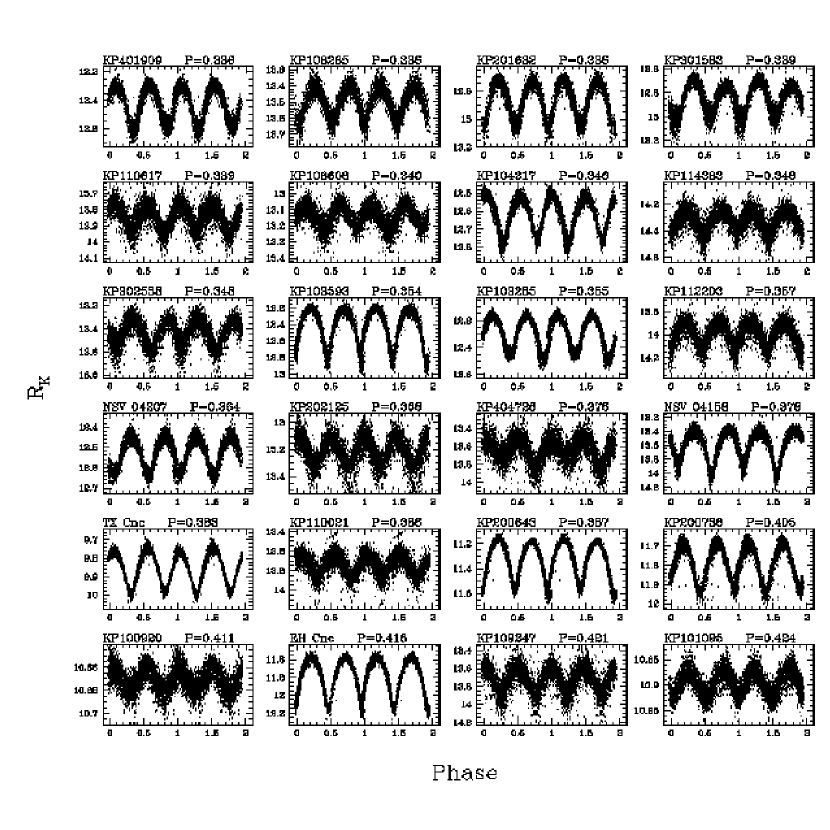
Figure 11: Lightcurves of eclipsing periodic variables identified by KELT, sorted by period.

Figure 12: Lightcurves of eclipsing periodic variables identified by KELT, sorted by period.

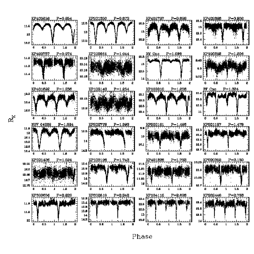
Figure 13: Lightcurves of eclipsing periodic variables identified by KELT, sorted by period.

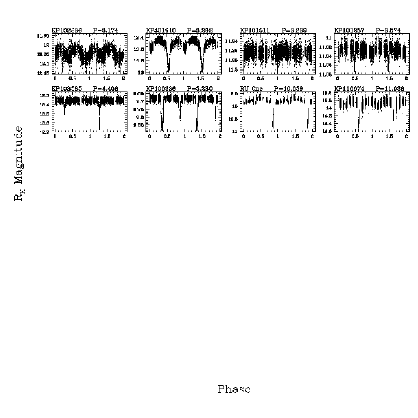
Figure 14: Lightcurves of eclipsing periodic variables identified by KELT, sorted by period.

Figure 15: Lightcurves of the four best transit candidates.

Figure 16: Spectroscopic orbit of transit candidate KP102791, with a period of $3.0227\pm 0.0011$ days. The amplitude of the orbit clearly indicates that the companion is a stellar companion and not a planet. This object turns out to be an eclipsing binary with a 1.5$M_{\odot}$ primary with a 0.75$M_{\odot}$ secondary.

References

- Adams et al. (2002) Adams, J. D., Stauffer, J. R., Skrutskie, M. F., Monet, D. G., Portegies Zwart, S. F., Janes, K. A., & Beichman, C. A. 2002, AJ, 124, 1570
- Alard & Lupton (1998) Alard, C. & Lupton, R.H. 1998, ApJ, 503, 325
- Alard (2000) Alard, C. 2000, A&A, 144, 363
- Alonso et al. (2004) Alonso, R., et al. 2004, ApJ, 613, L153
- An et al. (2007) An, D., Terndrup, D. M., Pinsonneault, M. H., Paulson, D. B., Hanson, R. B., & Stauffer, J. R. 2007, ApJ, 655, 233
- Bakos et al. (2004) Bakos, G., Noyes, R. W., Kovacs, G., Stanek, K. Z., Sasselov, D. D., & Domsa, I. 2004, PASP, 116, 266
- Bakos et al. (2007) Bakos, G. A. 2006, ApJ, 656, 552
- Barnes & Fortnoy (2004) Barnes, J. W. & Fortnoy, J. J. 2004, ApJ, 616, 1193
- Binney & Merrifield (1998) Binney, J. & Merrifield, M. 1998, Galactic Astronomy (Princeton: Princeton University Press)
- Burke et al. (2006) Burke, C. J., Gaudi, B. S., DePoy, D. L., & Pogge, R. W. 2006, AJ, 132, 210
- Burke et al. (2007) Burke, C. J., et al. 2007, submitted to ApJ, astro-ph/0705.0003
- Cameron et al. (2007) Cameron, A. C., et al. 2007, MNRAS, 375, 951
- Chappelle et al. (2005) Chappelle, R. J., Pinfield, D. J., Steele, I. A., Dobbie, P. D., & Magazzu, A. 2005, MNRAS, 361, 1323
- Charbonneau et al. (2002) Charbonneau, D., Brown, T. M., Noyes, R. W., & Gilliland, R. L. 2002, ApJ, 568, 377
- Charbonneau et al. (2007) Charbonneau, D., Brown, T. M., Burrows, A., & Laughlin, G. 2007, in Protostars & Planets V, ed. B. Reipurth, D. Jewitt, & K. Keil (Tucson: University of Arizona Press), 701
- Gaudi & Winn (2007) Gaudi B. S. & Winn, J. N. 2007, ApJ, 655, 550
- Guillot (2005) Guillot, T. 2005, Annual Review of Earth and Planetary Sciences, 33, 493
- Hartman et al. (2004) Hartman, J. D., Bakos, G., Stanek, K. Z., & Noyes, R. W. 2004, AJ, 128, 1761
- Høg et al. (2000) Høg, E., et al. 2000, A&A, 355, L27
- Jones & Stauffer (1991) Jones, B. F. & Stauffer, J. R. 1991, AJ, 102, 1080
- Kurucz (1992) Kurucz, R. L. 1992, IAUS, 149, 225
- Kaluzny et al. (1998) Kaluzny, J., Stanek, K. Z., Krockenberger, M., Sasselov, D. D., Tonry, J. L., & Mateo, M. 1998, AJ, 115, 1016
- Kovacs, Zucker, & Mazeh (2002) Kovacs, G., Zucker, S., & Mazeh, T. 2002, A&A, 391, 369
- Latham (1992) Latham, D. W. 1992, in IAU Coll. 135, Complementary Approaches to Double and Multiple Star Research, ASP Conf. Ser. 32, ed. H. A. McAlister & W. I. Hartkopf (San Francisco: ASP), 110
- Latham (2003) Latham, D. W. 2003, in ASP Conf. Ser. 294, Scientific Frontiers in Research on Extrasolar Planets, ed. D. Deming & S. Seager (San Francisco: ASP), 409
- Latham (2007) Latham, D. W. 2007, in ASP Conf. Ser. 366, Transiting Extrasolar Planet Workshop, ed. C. Afonso, D. Weldrake, & Th. Henning,
- Kukarkin et al. (1982) Kukarkin, B. V., et al. 1982, New Catalog of Suspected Variable Stars (Moscow: Nauka)
- Mazeh, Tamuz, & Zucker (2007) Mazeh, T., Tamuz, O., & Zucker, S. 2007, ASPC, 366, 119
- McCullough et al. (2006) McCullough, P. R., et al. 2006, ApJ, 648, 1228
- McCullough et al. (2005) McCullough, P. R., Stys, J. E., Valenti, J. A., Fleming, S. W., Janes, K. A., & Heasley, J. N. 2005, PASP, 117, 783
- O’Donovan et al. (2006) O’Donovan, F. T., et al. 2006, ApJ, 651L, 61
- O’Donovan et al. (2007) O’Donovan, F. T., et al. 2007, ApJ, 663L, 37
- Pepper, Gould, & DePoy (2003) Pepper, J., Pogge, R. W., & Depoy, D. L. 2003, Acta Astron, 53, 213
- Pepper et al. (2007) Pepper, J., Pogge, R. W., DePoy, D. L., Marshall, J. L., Stanek, K. Z., Stutz, A. M., Poindexter, S., Siverd, R., O’Brien, T. P., Trueblood, M., & Trueblood, P. 2007, submitted to AJ, astro-ph/0704.0460
- Pollacco et al. (2006) Pollacco, D. L., et al. 2006, PASP, 118, 1407
- Samus & Durlevich (2004) Samus, N. N. & Durlevich, O. V. 2004, Combined General Catalog of Variable Stars (ed. 4.2; Moscow: Sternberg Astron. Inst.)
- Schlegel, Finkbeiner, & Davis (1998) Schlegel, D. J. Finkbeiner, D. P., Davis, M. 1998, ApJ, 500, 525
- Schwarzenberg-Czerny (1996) Schwarzenberg-Czerny, A. 1996, ApJ, 460, L107
- Skrutskie et al. (2006) Skrutskie, M. F. 2006, AJ, 131, 1163
- Stetson (1987) Stetson, P. B. 1987, PASP, 99, 191
- Stetson (1996) Stetson, P. B. 1996, PASP, 108, 851
- Tamuz, Mazeh, & Zucker (2005) Tamuz, O., Mazeh, T., & Zucker, S. 2005, MNRAS, 356, 1466
- Udalski et al. (2002a) Udalski, A. et al. 2002, Acta Astron, 52, 1
- Udalski et al. (2002b) Udalski, A., Zebrun, K., Szymanski, M., Kubiak, M., Soszynski, I., Szewczyk, O., Wyrzykowski, L., Pietrzynski, G. 2002, Acta Astron, 52, 1
- Udalski et al. (2002c) Udalski, A., Szewczyk, O., Zebrun, K., Pietrzynski, G., Szymanski, M., Kubiak, M., Soszynski, I., Wyrzykowski, L. 2002, Acta Astron, 52, 317
- Udalski et al. (2003) Udalski, A., Pietrzynski, G., Szymanski, M., Kubiak, M., Zebrun, K., Soszynski, I., Szewczyk, O., Wyrzykowski, L. 2003, Acta Astron, 53, 133
- Udalski et al. (2004) Udalski, A., Szymanski, M. K., Kubiak, M., Pietrzynski, G., Soszynski, I., Zebrun, K., Szewczyk, O., Wyrzykowski, L. 2004, Acta Astron, 54, 313