Anisotropic step stiffness from a kinetic model of epitaxial growth

Abstract

Starting from a detailed model for the kinetics of a step edge or island boundary, we derive a Gibbs-Thomson type formula and the associated step stiffness as a function of the step edge orientation angle, $\theta$. Basic ingredients of the model are: (i) the diffusion of point defects (“adatoms”) on terraces and along step edges; (ii) the convection of kinks along step edges; and (iii) constitutive laws that relate adatom fluxes, sources for kinks, and the kink velocity with densities via a mean-field approach. This model has a kinetic (nonequilibrium) steady-state solution that corresponds to epitaxial growth through step flow. The step stiffness, ${\tilde{\beta}}(\theta)$, is determined via perturbations of the kinetic steady state for small edge Péclet number, $P$, which is the ratio of the deposition to the diffusive flux along a step edge. In particular, ${\tilde{\beta}}$ is found to satisfy ${\tilde{\beta}}=O(\theta^{-1})$ for $O(P^{1/3})<\theta\ll 1$, which is in agreement with independent, equilibrium-based calculations.

1 Introduction

The design and fabrication of novel small devices require the synergy of experiment, mathematical modeling and numerical simulation. In epitaxial growth, crystal surface features such as thin films, which are building blocks of solid-state devices, are grown on a substrate by material deposition from above. Despite continued progress, the modeling and simulation of epitaxial phenomena remains challenging because it involves reconciling a wide range of length and time scales.

An elementary process on solid surfaces is the hopping of atoms in the presence of line defects (“steps”) of atomic height [13, 22, 44]: atoms hop on terraces, and attach to and detach from step edges (or island boundaries). Burton, Cabrera and Frank (BCF) [6] first described each step edge as a boundary moving by mass conservation of point defects (“adatoms”) which diffuse on terraces. In the BCF theory, the step motion occurs near thermodynamic equilibrium. Subsequent theories have accounted for far-from-equilibrium processes; for a review see section 2.

The macroscale behavior of crystal surfaces is described by use of effective material parameters such as the step stiffness, ${\tilde{\beta}}$ [27]. In principle, ${\tilde{\beta}}$ depends on the step edge orientation angle, $\theta$, and is viewed as a quantitative measure of step edge fluctuations [1, 38]. Generally, effective step parameters such as ${\tilde{\beta}}$ originate from atomistic processes to which inputs are hopping rates for atoms; in practice, however, the parameters are often provided by phenomenology. For example, the dependence of ${\tilde{\beta}}$ on $\theta$ is usually speculated by invoking the underlying crystal symmetry [4, 19, 34, 35].

In this article we analyze a kinetic model for out-of-equilibrium processes [7, 8] in order to: (i) derive a Gibbs-Thomson (GT) type formula, which relates the adatom flux normal to a curved step edge and the step edge curvature [21, 22]; and (ii) determine the step stiffness ${\tilde{\beta}}$, which enters the GT relation, as a function of $\theta$. For this purpose, we apply perturbations of the kinetic (nonequilibrium) steady state of the model for small Péclet number $P$, which is the ratio of the material deposition flux to the diffusive flux along a step edge, i.e.

(1) $$P=(2a^{3}\bar{f})/D_{E}~{},$$

in which $a$ is an atomic length, $\bar{f}$ is a characteristic size for the flux $f$ normal to the boundary from each side, and $D_{E}$ is the coefficient for diffusion along the boundary. A factor of $2$ is included in (1) since the flux is two-sided and the total flux is of size $2\bar{f}$. For sufficiently small $\theta$ and $P$, we find that the stiffness has a behavior similar to that predicted by equilibrium-based calculations [37].

For the boundary of a two-dimensional material region, a definition of ${\tilde{\beta}}$ can arise from linear kinetics. In the setting of atom attachment-detachment at an edge, this theory states that the material flux, $f$, normal to the curved boundary is linear in the difference of the material density, $\rho$, at the boundary from a reference or “equilibrium” density, $\rho_{0}$. The GT formula connects $\rho_{0}$ to the boundary curvature, $\kappa$. For unit layer thickness and negligible step interactions [22], the normal flux reads

(2) $$f={D_{A}}(\rho-\rho_{0}),$$

where ${D_{A}}$ is the diffusion coefficient for attachment and detachment, and $\rho_{0}$ is defined by

(3) $$\rho_{0}=\rho_{*}\,e^{\frac{{\tilde{\beta}}\,\kappa}{k_{B}T}}\sim\rho_{*}\biggl{(}1+\frac{{\tilde{\beta}}}{k_{B}T}\,\kappa\biggr{)},\qquad|{\tilde{\beta}}\kappa|\ll k_{B}T~{}.$$

The last equation is referred to as the GT formula, in accord with standard thermodynamics [5, 17, 24, 26, 31]. In (3), $\rho_{*}$ is the equilibrium density near a straight step edge and $k_{B}T$ is Boltzmann’s energy ($T$ is temperature); the condition $|{\tilde{\beta}}\kappa|\ll k_{B}T$ is satisfied in most experimental situations [43]. Equation (2) does not account for step permeability, by which terrace adatoms hop directly to adjacent terraces [28, 41]. This process is discussed in section 2.

For systems that are nearly in equilibrium, the exponent in (3) is derived by a thermodynamic driving force starting from the step line tension $\beta$, the free energy per unit length of the boundary [18]. The step stiffness ${\tilde{\beta}}$ is related to $\beta$ by [1, 15, 16]

(4) $${\tilde{\beta}}=\beta+\beta_{\theta\theta}\qquad(\beta_{\theta}:=\partial_{\theta}\beta)~{}.$$

Evidently, the knowledge of ${\tilde{\beta}}$ alone does not yield $\beta$ uniquely: by (4),

(5) $$\beta(\theta)=C_{1}\,\cos\theta+C_{2}\,\sin\theta+\int_{0}^{\theta}d\vartheta\ {\tilde{\beta}}(\vartheta)\,\sin(\theta-\vartheta)$$

where $C_{1}$ and $C_{2}$ are in principle arbitrary constants.

The parameters $\beta$ and ${\tilde{\beta}}$ are important in the modeling and numerical simulation of epitaxial phenomena. In thermodynamic equilibrium, the angular dependence of the step line tension, $\beta(\theta)$, determines the equilibrium (two-dimensional) shape of step edges or islands, e.g. the macroscopic flat parts (“facets”) of the step are found by minimizing the step line energy through the Wulff construction [20, 29, 30, 40, 42, 45]. Near thermodynamic equilibrium, the step stiffness, ${\tilde{\beta}}(\theta)$, controls the temporal decay of fluctuations from equilibrium [1, 22]. The significance of ${\tilde{\beta}}$ was pointed out by de Gennes in the context of polymer physics almost forty years ago [10, 12]: the energy of a polymer (or step edge) can be described by a kinetic energy term proportional to ${\tilde{\beta}}\cdot(dx/dy)^{2}$, i.e., the stiffness times a “velocity” squared where $x$ and $y$ are suitable space coordinates and $y$ loosely corresponds to “time.” Starting with a two-dimensional Ising model, Stasevich et al. [36, 37, 38, 39] carried out a direct derivation of $\beta(\theta)$ and ${\tilde{\beta}}(\theta)$ from an equilibrium perspective based on atomistic key energies. For most systems, however, there has been no standard theoretical method for determining $\beta(\theta)$ and ${\tilde{\beta}}(\theta)$.

More generally, energetic principles such as a thermodynamic driving force are powerful as a means of describing the macroscopic effect of atomistic kinetics. The range of validity of energetic principles is not fully known and is an important unresolved issue. We believe that energetic arguments should be valid for systems that are nearly in local equilibrium, where the relevant processes approximately satisfy detailed balance. For systems that are far from equilibrium, however, energetic principles may serve as a valuable qualitative guide, even if they are not quantitatively accurate.

The kinetic and atomistic origin of a material parameter that plays the role of the step stiffness are the subject of this article. For a step edge or an island boundary on an epitaxial crystal surface, we use the detailed kinetic model formulated by Caflisch et al. [7, 8] and further developed by Balykov and Voigt [2, 3] for the dynamics of the boundary. The basic ingredients are: (i) diffusion equations for adatom and edge-atom densities on terraces and along step edges; (ii) a convection equation for the kink density along step edges; and (iii) constitutive, algebraic laws for adatom fluxes, sources for kinks and the kink velocity by mean-field theory. This model admits a kinetic (nonequilibrium) steady state that allows for epitaxial growth via step flow. The model has been partly validated by kinetic Monte Carlo simulations [7].

The detailed step model described in [7, 8] and section 2.3 focuses on the kinetics of adatoms, edge-atoms and kinks at a step edge. As discussed by Kallunki and Krug [23], an edge-atom is energetically equivalent to two kinks. For example, the equilibrium density of kinks is proportional to $\exp[-\varepsilon/(k_{B}T)]$ while the equilibrium density of edge-atoms is proportional to $\exp[-2\varepsilon/(k_{B}T)]$, in which $\varepsilon$ is defined as the kink energy in [23], or identified with $-(k_{B}T/2)\log({D_{K}/D_{E}})$ in [7]; $D_{K}$ and $D_{E}$ are diffusion coefficients for kinks and edge-atoms. On the other hand, the kinetics in [7, 8] are different for edge-atoms and kinks, since edge-atoms can hop at rate $D_{E}$, while kinks move through detachment of atoms at rate $D_{K}$. This situation is consistent with the kinetics described in [23], in which the $D_{E}$ and $D_{K}$ are proportional to $\exp[-E_{st}/(k_{B}T)]$ and $\exp[-E_{det}/(k_{B}T)]$, respectively.

We are aware that the mean-field laws applied here, although plausible and analytically tractable, pose a limitation: actual systems are characterized by atomic correlations, which can cause deviations from this mean-field approximation. In particular, the validity of the mean-field assumption may be limited to orientation angles $\theta$ in some neighborhood of $\theta=0$. Note also that the most interesting results of this analysis are for $\theta$ near zero. Determination of the range of validity for this model is an important endeavor but beyond the scope of this paper. An extension of this model, which could improve its range of validity, would be to explicitly track the kinks in a step edge. This additional discreteness in the model would make the analysis of step stiffness more difficult. Our analysis is a systematic study of predictions from the mean-field approach only, and the conclusions presented here are all derived within the context of this approach. On the other hand, our analysis is more detailed than previous treatments of step stiffness, since it is based on kinetics rather than a thermodynamic driving force. Moreover, the model includes atomistic information, through a density of adatoms, edge-atoms and kinks.

For evolution near the kinetic steady state, we derive for the mass flux, $f$, a term analogous to the Gibbs-Thomson formula (3), and subsequently find the corresponding angular dependence of the step stiffness, ${\tilde{\beta}}(\theta)$. Our main assumptions are: (i) the motion of step edges or island boundaries is slower than the diffusion of adatoms and edge-atoms and the convection of kinks, which amounts to the “quasi-steady approximation”; (ii) the mean step edge radius of curvature, $\kappa^{-1}$, is large compared to other length scales including the step height, $a$; and (iii) the edge Péclet number, $P$, given by (1) is sufficiently small, which signifies the usual regime for molecular beam epitaxy (MBE). To the best of our knowledge, the analysis in this paper offers the first kinetic derivation of a Gibbs-Thomson type relation and the step stiffness for all admissible values of the step edge orientation angle, $\theta$. (This approach is distinctly different from the one in e.g. [33] where classical elasticity is invoked.) Our results for the stiffness are summarized in section 3; see (41)–(53).

A principal result of our analysis is that ${\tilde{\beta}}=O(\theta^{-1})$ for $O(P^{1/3})<\theta\ll 1$, which by (5) yields $\beta=O(\theta\ln\theta)$ for the step line tension. This result is in agreement with the independent analysis in [36, 37, 38, 39], which makes use of equilibrium concepts. A detailed comparison of the two approaches is not addressed in our analysis. Our findings are expected to have significance for epitaxial islands, for example in predicting their facets, their roughness (e.g., fractal or smooth island boundaries) and their stability, as well as for the numerical simulation of epitaxial growth. More generally, our analysis can serve as a guide for kinetic derivations of the GT relation in other material systems. For example, it should be possible to derive the step stiffness for a step in local thermodynamic equilibrium within the context of the same model. This topic is discussed briefly in section 6.

The present work extends an earlier analysis by Caflisch and Li [8], which addressed the stability of step edge models and the derivation of the GT relation. The analysis in [8], however, only determined the value of ${\tilde{\beta}}$ along the high-symmetry orientation, $\theta=0$. This restriction was due to a scaling regime used in [8] on the basis of mathematical rather than physical principles. In the present article we transcend the analytical limitations of [8] by applying perturbation theory guided by the physics of the step-edge evolution near the kinetic steady state.

Our analysis also leads to formulas for kinetic rates in boundary conditions involving adatom fluxes. In particular, the attachment-detachment rates are derived as functions of the step edge orientation, and are shown to be different for up- and down-step edges. This asymmetry amounts to an Ehrlich-Schwoebel (ES) effect [11, 32], due to geometric effects rather than a difference in energy barriers. In addition, if the terrace adatom densities are treated as input parameters, the adatom fluxes involve effective permeability rates, by which a fraction of adatoms directly hop to adjacent terraces (without attaching to or detaching from step edges) [14, 28, 41]. Our main results for the kinetic rates are described by (35)–(39).

In this article we do not address the effects of elasticity, which are due for instance to bulk stress. One reason is that elasticity requires a non-trivial modification of the kinetic model that we use here. This task lies beyond our present scope. Another reason is that, in many physically interesting situations, the influence of elasticity may be described well via long-range step-step interactions that do not affect the step stiffness. The study of elastic effects is the subject of work in progress.

The remainder of this article is organized as follows. In section 2 we review the relevant island dynamics model and the concept of step stiffness: In section 2.1 we introduce the step geometry; in section 2.2 we outline elements of the BCF model, which highlight the GT formula; in section 2.3 we describe the previous kinetic, nonequilibrium step-edge model [7, 8], which is slightly revised here; and in section 2.4 we outline our program for the stiffness, based on the perturbed kinetic steady state for small step edge curvature, $\kappa$. In section 3 we provide a summary of our main results. In section 4 we derive analytic formulas pertaining to the kinetic steady state: In section 4.2 we use the mass fluxes as inputs and derive the ES effect [11, 32]; and in section 4.3 we use the mass densities as inputs to derive asymmetric, $\theta$-dependent step-edge permeability rates. In section 5 we apply perturbation theory to find ${\tilde{\beta}}(\theta)$ by using primarily the mass fluxes as inputs: In section 5.1 we carry out the perturbation analysis to first order for the edge-atom and kink densities as $\kappa\to 0$; in section 5.3 we derive the step stiffness as a function of $\theta$; and in section 5.4 we discuss an alternative viewpoint on the stiffness. In section 6 we discuss our results, and outline possible limitations. The appendices provide derivations and proofs needed in the main text.

2 Background

In this section we provide the necessary background for the derivation of the step stiffness. First, we describe the step configuration. Second, we revisit briefly the constituents of the BCF theory with focus on the GT formula and the step stiffness, ${\tilde{\beta}}$. Our review provides the introduction of ${\tilde{\beta}}$ from a kinetic rather than a thermodynamic perspective. Third, we describe in detail the nonequilibrium kinetic model [7, 8] with emphasis on the mean-field constitutive laws for edge-atom and kink densities. Fourth, we set a perturbation framework for the derivation of ${\tilde{\beta}}(\theta)$.

2.1 Step geometry and conventions

Following [7, 8] we consider a simple cubic crystal (solid-on-solid model) with lattice spacing $a$ and crystallographic directions identified with the $x$, $y$ and $z$ axes of the Cartesian system. The analysis of this paper is for a step edge or island boundary to which there is flux $f$ of atoms from the adjoining terraces. The flux $f$ may vary along the edge, as well as in time, and it comes from both sides of the edge, but it is characterized by a typical size $\bar{f}$ which has units of $(length\cdot time)^{-1}$. In [7, 8] the geometry was specialized to a step train with interstep distance $2L$ and deposition flux $F$, so that in steady state the flux to the step is $f=LF$. This global scenario is not necessary, however, since the analysis here is local and only requires a nonzero quasi-steady flux $f$. This could occur even with no deposition flux $F=0$; for example, in annealing.

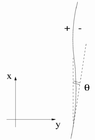
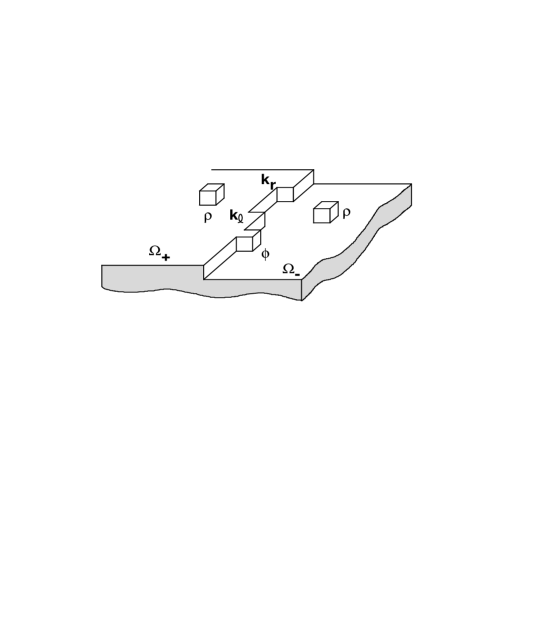
Fig. 1: The macroscopic (left) and microscopic (right) views of a step edge in the (high-symmetry) $xy$-plane of a crystal. In the macroscopic view, the step edge orientation relative to the $x$ axis is indicated by the angle $\theta$. The $+$ ($-$) sign indicates an upper (lower) terrace. The surface height decreases to the right. The microscopic view shows adatoms ($\rho$), edge-atoms ($\phi$), left-facing kinks ($k_{\ell}$) and right-facing kinks ($k_{r}$); $\Omega_{+}$ ($\Omega_{-}$) is the region of the upper (lower) terrace.

For algebraic convenience we adopt and extend the notation conventions of [8]. Specifically, we use the following symbols: ($x,y,z$) for dimensional spatial coordinates, $t$ for time, $D$ for any diffusion coefficient, $\rho$ for number density per area , and $\xi$ for number density per length; and define the corresponding nondimensional quantities $\tilde{x},\tilde{y},\tilde{z},\tilde{t},\tilde{D},\tilde{\rho},\tilde{\xi}$ by

(6) $$(\tilde{x},\tilde{y},\tilde{z}) := (x/a,y/a,z/a)~{},$$

(7) $$\tilde{t} := (a\bar{f})\,t~{},$$

(8) $$\tilde{D} := D/(a^{3}\bar{f})~{},$$

(9) $$\tilde{\rho} := a^{2}\rho~{},$$

(10) $$\tilde{\xi} := a\xi~{}.$$

Now drop the tildes, so that $x,y,z,t,D,\rho,\xi$ are dimensionless. This choice amounts to measuring all distances in units of $a$ and all times in units of $(a\bar{f})^{-1}$. Equivalently, (6)–(10) correspond to setting $a=1$ and $\bar{f}=1$. For our analysis, the single most important dimensionless parameter is the Peclet number $P$ from (1), which is equal to $2D_{E}^{-1}$ after nondimensionalization; i.e.

(11) $$D_{E}=2P^{-1}.$$

Next, we describe the coordinates of the step geometry in more detail. We consider step boundaries that stem from perturbing a straight step edge coinciding with a fixed axis (e.g., the $x$-axis). All steps are parallel to the high-symmetry (“basal”), $xy$-plane of the crystal. The projection of each edge on the basal plane is represented macroscopically by a smooth curve with a local tangent that forms the (signed) angle $\theta$ with the $x$-axis, where $-\theta_{0}<\theta<\theta_{0}$ . Without loss of generality we take $0\leq\theta<\theta_{0}$ and assume that $\theta_{0}<\pi/4$ in our analysis. We take the upper terrace to be to the left of an edge so that all steps move to the right during the growth process. So, the projection of each step edge is represented by

(12) $$y=Y(x,t)~{},$$

where $Y(x,t)$ is a sufficiently differentiable function of ($x,t$).

It follows that the unit normal and tangential vectors to the step boundary are [8]

(13) $${\hat{\bf n}}=(\sin\theta,-\cos\theta)=(y_{s},-x_{s})~{},\qquad{\hat{}\mbox{\boldmath{$\tau$}}}=(\cos\theta,\sin\theta)=(x_{s},y_{s})~{},$$

where $s$ is the arc length and lowercase subscripts denote partial differentiation (e.g., $x_{s}:=\partial_{s}x$) unless it is noted or implied otherwise. The step edge curvature is

(14) $$\kappa=-\theta_{s}~{}.$$

There is one more geometric relation that deserves attention. By denoting the densities of left- and right-facing kinks $k_{l}$ and $k_{r}$, respectively, we have [7]

(15) $$k_{r}-k_{l}=-\tan\theta~{};$$

see section 2.3 for further discussion. This geometric relation poses a constraint on the total kink density, $k$ ($k\geq 0$). By

(16) $$k:=k_{r}+k_{l}$$

and (15), $k$ must satisfy

(17) $$k\geq|\tan\theta|~{}.$$

The formulation of a nonequilibrium kinetic step edge model (section 2.3) requires the use of several coordinate systems for an island boundary; these are described in appendix A. In the following analysis it becomes advantageous to use $\theta$ as the main local coordinate. Its importance as a dynamic variable along a step edge is implied by the steady-state limit $k\to|\tan\theta|$ as $\kappa\to 0$ and $P\to 0$; see (54). Some useful identities that enable transformations to the $(\theta,t)$ variables are provided in appendix A.

2.2 BCF model

In the standard BCF theory [6] the projection of step edges on the basal plane are smooth curves that move by the attachment and detachment of atoms due to mass conservation. The BCF model comprises the following near-equilibrium evolution laws. (i) The adatom density solves the diffusion equation on terraces. (ii) The adatom flux and density satisfy (kinetic) boundary conditions for atom attachment-detachment at step edges. (iii) The step velocity equals the sum of the adatom fluxes normal to the edge. In this setting, the GT formula links the normal mass flux to the step edge curvature.

We next describe the equations of motion in the BCF model for comparisons with the kinetic model of section 2.3. The density, $\rho$, of adatoms on each terrace solves

(18) $$\partial_{t}\rho-{D_{T}}\,\Delta\rho=F~{},$$

where ${D_{T}}$ is the terrace diffusion coefficient and $\Delta$ denotes the Laplacian in $(x,y)$.

As an extension of the BCF model, the boundary conditions for (18) are now formulated by linear kinetics with inclusion of both atom attachment-detachment and step permeability [22, 28, 41]:

(19) $$f_{\pm}={D_{A}}^{\pm}\,(\rho_{\pm}-\rho_{0}^{\pm})\pm D_{p}^{\pm}\,(\rho_{+}-\rho_{-})~{};$$

cf. (2). Here, $f_{\pm}$ is the adatom flux normal to an edge from the upper ($+$) or lower ($-$) terrace, i.e.,

(20) $$\mp f_{\pm}:=v\rho_{\pm}+{D_{T}}{\hat{\bf n}}\cdot(\nabla\rho)_{\pm}~{},$$

$\rho_{\pm}$ is the terrace adatom density restricted to the step edge, ${D_{A}}^{\pm}$ is the attachment-detachment rate coefficient and $D_{p}^{\pm}$ is the permeability rate coefficient. These rates can account for different up- and down-step energy barriers, e.g. the ES effect in the case of ${D_{A}}^{\pm}$ [11, 32]. The reference density $\rho_{0}^{\pm}$ is given by (3) where $\rho_{*}$ is replaced by $\rho_{*}^{\pm}$ for up- and down-step edge asymmetry. Evidently, (19) forms an extension of formula (2) but still corresponds to near-equilibrium kinetics; it will be modified in section 2.3.

Equations (18) and (19) provide the fluxes $f_{\pm}$ as functions of the step edge position and curvature. The step velocity, $v$, is then determined by mass conservation,

(21) $$v=f_{+}+f_{-}~{}.$$

In this formulation, step-edge diffusion and kink motion are neglected. In the next section, the BCF model is enriched with kinetic boundary conditions that account for the motion of edge-atoms and kinks.

2.3 Atomistic, nonequilibrium kinetic model

In this section we revisit the kinetic model by Caflisch et al. [7, 8], which is an extension of the BCF model (section 2.2) to nonequilibrium processes. We apply this kinetic model [7] to step edges of arbitrary orientation; and further revise it to account for a step edge diffusion coefficient defined along the (fixed) crystallographic $x$-axis. This last feature, although not important for our present purpose of calculating the step stiffness, renders the model consistent with recent studies of the edge-atom migration along a step edge [23]. The following processes are included. (i) Adatom diffusion on terraces, which is described by (18) of the BCF theory, and edge-atom diffusion along step edges. (ii) Convection of kinks on step edges with sinks and sources to account for conversion of terrace adatoms and edge-atoms to kinks. (iii) Constitutive laws that relate mass fluxes, sources for kinks and the step velocity with densities via a mean-field theory, and modify the BCF laws (19) and (21). In this model, kink densities are assumed sufficiently small, enabling the neglect of higher-order terms within the mean-field approach. Recently, extensions of this theory were developed [2, 3, 14], including higher kink densities by Balykov and Voigt [2, 3]. Next, we state the requisite equations of motion in addition to (18) for adatom terrace diffusion.

2.3.1 Equations of motion along step edges

An assumption inherent to the present model is the different kinetics of kinks and edge-atoms. Each of these species is of course not conserved separately, since edge-atoms can generate kinks, but can be described by a distinct density: $\phi(x,t)$ for edge-atoms and $k(x,t)$ for kinks. In addition, their motion is different: the edge-atom flux follows from gradients of the density $\phi$; while the kink flux stems from a velocity field, $w$.

We proceed to describe the equations of motion. The edge-atom number density, $\phi(x,t)$, solves

(22) $$\partial_{t}\phi-{D_{E}}\,\partial_{x}^{2}\phi=\frac{f_{+}+f_{-}}{\cos\theta}-f_{0}~{},$$

where ${D_{E}}$ is the step edge diffusivity defined along the high-symmetry ($x$-) axis and $f_{0}$ represents the loss of edge-atoms to kinks; see (26) and (32) below. For later algebraic convenience, it is advantageous to transform (22) to $(\theta,t)$ variables. By the formulas  (133) and (138) of appendix A, (22) is thus recast to

(23) $$\partial_{t}|_{\theta}\phi+\kappa(v_{\theta}+v\tan\theta)\partial_{\theta}\phi-{D_{E}}\frac{\kappa}{\cos\theta}\partial_{\theta}\frac{\kappa}{\cos\theta}\partial_{\theta}\phi=\frac{f_{+}+f_{-}}{\cos\theta}-f_{0}~{}.$$

We turn our attention to kinks. The total kink density, $k(x,t)$, of (16) solves

(24) $$\partial_{t}k+\partial_{x}[w(k_{r}-k_{l})]=2(g-h)~{},$$

where $w(k_{r}-k_{l})=-w\tan\theta$ is the flux of kinks with respect to the $x$-axis, $g$ is the net gain in kink pairs due to nucleation and breakup, and $h$ is the net loss in kink pairs due to creation and annihilation [7]. The terms $w$, $g$ and $h$ are described as functions of densities in (28)–(30) below. In the $(\theta,t)$ coordinates, (24) reads

(25) $$\partial_{t}|_{\theta}k+\kappa(v_{\theta}+v\tan\theta)\partial_{\theta}k+\frac{\kappa}{\cos\theta}\partial_{\theta}(w\tan\theta)=2(g-h)~{}.$$

Equations (22) and (24) can be transformed to other coordinates, including the $(s,t)$ variables where $s$ is the arc length. For completeness, in appendix B we provide relations that are needed in such transformations; and in appendix C we describe the ensuing equations of motion in the $(s,t)$ coordinates.

Partial differential equations (22) and (24) are coupled with the motion of step edges. In the following analysis, we apply the quasi-steady approximation, neglecting the time derivative in (23) and (25). For definiteness, the boundary conditions in $x$ can be taken to be periodic. It remains to prescribe boundary conditions for atom attachment-detachment, i.e., specify $f_{\pm}$ in (20). In the present nonequilibrium context, $f_{\pm}$ are no longer given by (19) of the BCF model, as discussed next.

2.3.2 Constitutive laws

Following [7, 8] we describe mean-field constitutive laws for fluxes related to a tilted step edge (at $\theta\neq 0$). We also provide a geometric relation for the step edge velocity, $v$, which in a certain sense replaces the BCF law (21). Because the explanations are given elsewhere [2, 7], we state the mean-field laws without a detailed discussion of their origin.

By mean-field theory, the terrace adatom flux normal to the step edge is [7]

(26) $$f_{\pm} = [{D_{T}}\rho_{\pm}-{D_{E}}\phi+l_{j_{\pm}}({D_{T}}\rho_{\pm}-D_{K})k+m_{j_{\pm}}({D_{T}}\rho_{\pm}\phi-D_{K}k_{r}k_{l})$$

$$+n_{j_{\pm}}({D_{T}}\rho_{\pm}k_{r}k_{l}-D_{B})]\cos\theta,\quad j_{+}=2,\ j_{-}=3~{},$$

where $l_{j}$, $m_{j}$ and $n_{j}$ are (effective) coordination numbers (positive integers) that count the number of possible paths in the kinetic processes, weighted by the relative probability of a particle to be at the corresponding position. Also, $D_{K}$ is the diffusion coefficient for an atom from a kink, and $D_{B}$ is the diffusion coefficient for an atom from a straight edge. By neglect of $D_{K}$ and $D_{B}$, (26) readily becomes

(27) $$f_{\pm}=(1+l_{j_{\pm}}k+m_{j_{\pm}}\phi+n_{j_{\pm}}k_{r}k_{l}){D_{T}}\rho_{\pm}\cos\theta-D_{E}\phi\cos\theta~{}.$$

Omitting $D_{K}$ and $D_{B}$ is inconsistent with detailed balance, but has little effect on the kinetic solutions described below.

Similarly, the mean-field kink velocity reads [7]

(28) $$w=l_{1}{D_{E}}\phi+{D_{T}}(l_{2}\rho_{+}+l_{3}\rho_{-})-l_{123}D_{K}\sim l_{1}{D_{E}}\phi+{D_{T}}(l_{2}\rho_{+}+l_{3}\rho_{-})~{}.$$

The gain in kink pairs from nucleation and breakup involving an edge-atom is [7]

(29) $$g = \phi(m_{1}{D_{E}}\phi+m_{2}{D_{T}}\rho_{+}+m_{3}{D_{T}}\rho_{-})-m_{123}\,D_{K}k_{r}k_{l}$$

$$\sim \phi(m_{1}{D_{E}}\phi+m_{2}{D_{T}}\rho_{+}+m_{3}{D_{T}}\rho_{-})~{}.$$

The respective loss of kink pairs by atom attachment-detachment is [7]

(30) $$h = (n_{1}{D_{E}}\phi+n_{2}{D_{T}}\rho_{+}+n_{3}{D_{T}}\rho_{-})k_{r}k_{l}-n_{123}\,D_{B}$$

$$\sim (n_{1}{D_{E}}\phi+n_{2}{D_{T}}\rho_{+}+n_{3}{D_{T}}\rho_{-})k_{r}k_{l}~{}.$$

In the above,

(31) $$p_{ij}:=p_{i}+p_{j},\quad p_{ijk}:=p_{i}+p_{j}+p_{k};\qquad p=m,\,n,\,l~{}.$$

The constitutive laws are complemented by

(32) $$f_{0}=wk+2g+h~{},$$

which enters (23). The step edge velocity, $v$, stems from a geometric relation; see appendix D for details. Specifically,

(33) $$v=\frac{f_{0}}{1+\phi\kappa\cos\theta}\cos\theta=\frac{wk+2g+h}{1+\phi\kappa\cos\theta}\cos\theta~{}.$$

2.4 Program for step stiffness

In this section we delineate a program for the calculation of the step stiffness from the model of section 2.3. The key idea is to reduce the nonequilibrium law (26) to the linear kinetic law (19) by treating the normal fluxes, $f_{\pm}$, as external, free to vary, $O(1)$ parameters of the equations of motion along a step edge. In this context, the diffusion equation (18) is not invoked. Our method relies on the perturbation of a solution for the densities $\phi$ and $k$. The solution studied here is that of the kinetic steady state, under the assumption that it can be reached. Accordingly, we neglect the time derivative in the zeroth-order equations of motion; furthermore, we neglect this derivative to the next higher order by imposing the quasi-steady approximation. Another case, left for future work, is that of thermodynamic equilibrium; see section 6. In summary, we apply the following procedure:

(i) To extract the kinetic steady state, we set $\partial_{t}|_{\theta}\equiv 0$ and $\kappa=0$ (i.e., we consider straight edges). This leads to a system of algebraic equations for $(\phi,k)\equiv(\phi^{(0)},k^{(0)})$ . The coefficients of this system depend on $\theta$ and $f_{\pm}$. In principle, $(\phi^{(0)},k^{(0)})$ cannot be found in simple closed form at this stage.

(ii) We assume that $P\ll 1$, and determine relatively simple expansions for $(\phi^{(0)},k^{(0)})$ in powers of $P$ for $0\leq\theta<O(P^{1/3})$ and $O(P^{1/3})<\theta<\pi/4$.

(iii) We replace $(\phi,k)$ by $(\phi^{(0)},k^{(0)})$ in the constitutive law (26) and compare the result to (19). Here, our analysis follows up two mathematically equivalent but physically distinct routes. (a) By taking $f_{\pm}$ as input parameters, we derive formulas for the adatom reference densities, $\rho_{*}^{\pm}$, and attachment-detachment rates, ${D_{A}}^{\pm}$, that depend on $f_{\pm}$; cf. (19). Step permeability is not manifested in this setting ($D_{p}\equiv 0$). (b) By considering $\rho_{\pm}$ as inputs, we predict attachment-detachment rates and non-vanishing step permeability rates.

(iv) We consider perturbations of the kinetic steady state by taking $0<|\kappa|\ll 1$, i.e. slightly curved step edges. Accordingly, we let

(34) $$\phi\sim\phi^{(0)}+\phi^{(1)}\,\kappa~{},\quad k\sim k^{(0)}+k^{(1)}\,\kappa~{},$$

where $\kappa\phi^{(1)}$ and $\kappa k^{(1)}$ are deviations from the kinetic steady state and depend on $(\phi^{(0)},k^{(0)})$. Expansion (34) is imposed on physical rather than mathematical grounds. Indeed, if the mean-field flux (26) is expected to reduce to the linear kinetic law (19), then $\phi$ must be linear in $\kappa$. The equations of motion along an edge and the constitutive laws are linearized in $\kappa\phi^{(1)}$ and $\kappa k^{(1)}$.

(v) By treating $f_{\pm}$ as input external parameters, we replace $\phi$ and $k$ in the right-hand side of the constitutive law (27) by expansions (34). Subsequently, we determine the stiffness ${\tilde{\beta}}(\theta;f_{+},f_{-})$ by comparison to (19) in view of (3).

The choice of fluxes $f_{\pm}$ or densities $\rho_{\pm}$ as input parameters is a physics modeling question. Although the mathematical results are equivalent for the two choice, the physical interpretation of these results is different, as stated above.

3 Main results

Here, we give the main formulas stemming from our analysis of the kinetic model described in section 2.3. A necessary condition for our perturbation analysis is $0\leq\kappa<O(P)\ll 1$, to be shown via a plausibility argument in section 5.1. Derivations and other related details are provided in sections 4 and 5.

3.1 ES effect (section 4.2)

When the fluxes $f_{\pm}$ are input parameters, the attachment-detachment of adatoms from a terrace to an edge is asymmetric. So, the related diffusion coefficients ${D_{A}}^{\pm}$, or attachment and detachment kinetic rates, which enter (19), are found to be different for an upper and lower terrace:

$${D_{A}}^{+} = {D_{T}}\bigl{[}1+l_{2}k^{(0)}+m_{2}\phi^{(0)}+\textstyle{\frac{1}{4}}n_{2}({k^{(0)}}^{2}-\tan^{2}\theta)\bigr{]}\cos\theta~{},$$

(35) $${D_{A}}^{-} = {D_{T}}\bigl{[}1+l_{3}k^{(0)}+m_{3}\phi^{(0)}+\textstyle{\frac{1}{4}}n_{3}({k^{(0)}}^{2}-\tan^{2}\theta)\bigr{]}\cos\theta~{},$$

where $0\leq\theta<\pi/4$ and $(l_{2},m_{2},n_{2})\neq(l_{3},m_{3},n_{3})$. For $0<P\ll 1$, we show that (35) reduce to

(36) $${D_{A}}^{\pm}\sim{D_{T}}(1+l_{j_{\pm}}\tan\theta)\cos\theta~{},$$

where $j_{+}=2$ and $j_{-}=3$. In this description, there is no step permeability. Note that the results presented in this section and their derivations do not depend on the step edge curvature.

3.2 Step permeability (section 4.3)

By using the adatom densities $\rho_{\pm}$ as input external parameters, we show that step permeability coexists with the ES effect; cf. (19). For $O(P^{1/3})<\theta<\pi/4$ the diffusion coefficients for permeability are

(37) $$D_{p}^{\pm}={D_{T}}\,\frac{A_{\mp}(1+l_{j_{\pm}}\tan\theta)}{1+(A_{+}+A_{-})\cos\theta}\cos^{2}\theta~{}.$$

The accompanying (asymmetric) attachment-detachment diffusion coefficients are

(38) $${D_{A}}^{\pm}={D_{T}}\frac{1+l_{j_{\pm}}\tan\theta\pm A_{\mp}(l_{2}-l_{3})\sin\theta}{1+(A_{+}+A_{-})\cos\theta}\cos\theta~{},$$

where

(39) $$A_{+}=\frac{1}{\sin\theta}\,\frac{1+l_{3}\tan\theta}{Q({\bf l})}~{},\qquad A_{-}=\frac{1}{\sin\theta}\,\frac{1+l_{2}\tan\theta}{Q({\bf l})}~{},$$

(40) $$Q({\bf p})=p_{1}(1+l_{2}\tan\theta)(1+l_{3}\tan\theta)+p_{2}(1+l_{3}\tan\theta)+p_{3}(1+l_{2}\tan\theta)~{},$$

with ${\bf p}:=(p_{1},\,p_{2},\,p_{3})$ and $p=l,\,m,\,n$; in (39), ${\bf l}=(l_{1},\,l_{2},\,l_{3})$. Note that $D_{p}^{\pm}$ and ${D_{A}}^{\pm}$ here are independent of $f_{\pm}$, as in (36). The corresponding results for $0\leq\theta<O(P^{1/3})$ are presented in section 4.3. Again, the results presented in this section and their derivations do not depend on the step edge curvature.

3.3 Step stiffness (section 5.3)

Let the adatom fluxes $f_{\pm}$ from an upper ($+$) and lower ($-$) terrace towards an edge be the input, independent parameters. For sufficiently small angle $\theta$, the stiffness is found to be

(41) $$\frac{{\tilde{\beta}}}{k_{B}T}\sim 2\frac{l_{123}}{n_{123}}\,\frac{(f_{+}+f_{-})_{\theta}}{f_{+}+f_{-}}\,\frac{1}{\theta}=O\biggl{(}\frac{1}{\theta}\biggr{)}\qquad O(P^{1/3})<\theta\ll 1~{},$$

(42) $$\frac{{\tilde{\beta}}}{k_{B}T}\sim P^{-2/3}\,\frac{4l_{123}}{n_{123}(\check{C}^{k}_{0})^{2}+8m_{123}}=O(P^{-2/3})\qquad 0\leq\theta<O(P^{1/3})\ll 1~{},$$

where $p_{123}$ ($p=l,\,m,\,n$) is defined in (31) and 

(43) $$\check{C}^{k}_{0}=\biggl{[}\frac{2m_{123}}{n_{123}\,l_{123}}(f_{+}+f_{-})\biggl{]}^{1/3}~{}.$$

Matching the asymptotic results (41) and (42) is discussed near the end of section 5.1.

For $\theta=O(1)$ the formula for ${\tilde{\beta}}$ becomes more complicated; we give it here for completeness. Generally,

(44) $$\frac{{\tilde{\beta}}}{k_{B}T}=\frac{\phi^{(1)}}{\phi^{(0)}}~{},$$

where $\phi^{(0)}$ and $\phi^{(1)}$ are expansion coefficients for $\phi$ and depend on $f_{\pm}$ and their derivatives in $\theta$; cf. (34). These coefficients are obtained explicitly for $P\ll 1$. In particular, for $O(P^{1/3})<\theta<\pi/4$,

(45) $$\phi^{(0)}\sim C^{\phi}_{0}\,P~{},\qquad\phi^{(1)}\sim C^{\phi}_{1}\,P~{},$$

(46) $$C^{\phi}_{0}=\frac{1}{2\sin\theta}\,\frac{(1+l_{3}\tan\theta)f_{+}+(1+l_{2}\tan\theta)f_{-}}{Q({\bf l})}~{},$$

(47) $$C^{\phi}_{1}=\frac{(v^{(0)}_{\theta}+v^{(0)}\tan\theta)k^{(0)}_{\theta}\cos\theta+(w^{(0)}\tan\theta)_{\theta}}{2\sin\theta}\,\frac{W^{k}\tan\theta+w^{(0)}+H^{k}}{H^{k}\,W^{\phi}}~{},$$

(48) $$v^{(0)}=f_{+}+f_{-}~{},$$

(49) $$w^{(0)}\sim 2l_{1}C^{\phi}_{0}+l_{2}\frac{s_{x}f_{+}+2C^{\phi}_{0}}{1+l_{2}\tan\theta}+l_{3}\frac{s_{x}f_{-}+2C^{\phi}_{0}}{1+l_{3}\tan\theta}~{},\qquad s_{x}=(\cos\theta)^{-1}~{},$$

(50) $$W^{\phi}=2l_{1}+\frac{2l_{2}}{1+l_{2}\tan\theta}+\frac{2l_{3}}{1+l_{3}\tan\theta}~{},$$

(51) $$W^{k}=-l_{2}\frac{l_{2}+\textstyle{\frac{n_{2}}{2}}\tan\theta}{(1+l_{2}\tan\theta)^{2}}(s_{x}f_{+}+2C^{\phi}_{0})-l_{3}\frac{l_{3}+\textstyle{\frac{n_{3}}{2}}\tan\theta}{(1+l_{3}\tan\theta)^{2}}(s_{x}f_{-}+2C^{\phi}_{0})~{},$$

(52) $$H^{k}=\frac{\tan\theta}{2}\biggl{(}2n_{1}C^{\phi}_{0}+n_{2}\,\frac{s_{x}f_{+}+2C^{\phi}_{0}}{1+l_{2}\tan\theta}+n_{3}\,\frac{s_{x}f_{-}+2C^{\phi}_{0}}{1+l_{3}\tan\theta}\biggr{)}~{},$$

(53) $$k\sim k^{(0)}\sim\tan\theta~{},$$

where $n_{j}$ and $l_{j}$ are coordination numbers. Recall definition (40) for $Q({\bf l})$. It is worthwhile noting that there is no asymmetry in the step stiffness $\tilde{\beta}$, in contrast to the attachment-detachment coefficients. The reason for this difference is that $\tilde{\beta}$ depends only on the edge-atom density, as shown in (44).

For the alternative approach in which the adatom densities $\rho_{\pm}$ are specified rather than the fluxes $f_{\pm}$, the analysis of the step stiffness is presented in section 5.4. The corresponding result (123) is not of the form (2) and (3), however, since the coefficient ß in (124) is not proportional to $\rho_{*}$.

4 The kinetic steady state

We analyze the kinetic steady state for a straight step, including its dependence on the Péclet number $P$ in section 4.1 and the ES effect and step permeabiity in sections 4.2 and 4.3.

4.1 Kinetic steady state and its dependence on $P$

In this section, we simplify the equations of motion for edge-atom and kink densities by imposing the kinetic steady state ($\partial_{t}\equiv 0$) for straight steps ($\kappa\equiv 0$). We find closed-form solutions for small Péclet number, $P\ll 1$, in two distinct ranges of $\theta$. For $\theta_{c}=O(P^{1/3})<\theta<\pi/4$, we show that $\phi=\phi^{(0)}$ is given by (45), and $k=k^{(0)}$ is given by (53), or more precisely by

(54) $$k^{(0)}\sim\tan\theta+C_{0}^{k}\,P,~{}$$

where

(55) $$C_{0}^{k}=\frac{2C_{0}^{\phi}}{\tan\theta}\frac{2C_{0}^{\phi}Q({\bf m})\cos\theta+m_{2}(1+l_{3}\tan\theta)f_{+}+m_{3}(1+l_{2}\tan\theta)f_{-}}{2C_{0}^{\phi}Q({\bf n})\cos\theta+n_{2}(1+l_{3}\tan\theta)f_{+}+n_{3}(1+l_{2}\tan\theta)f_{-}}~{};$$

$Q({\bf p})$ and $C_{0}^{\phi}$ are defined by (40) and (46). Furthermore,

(56) $$\phi^{(0)}\sim\check{C}^{\phi}_{0}\,P^{2/3}~{},\quad k^{(0)}\sim\check{C}^{k}_{0}\,P^{1/3}\qquad 0\leq\theta<\theta_{c}=O(P^{1/3})~{},$$

where $\check{C}^{k}_{0}$ is defined by (43),

(57) $$\check{C}^{\phi}_{0}=\biggl{(}\frac{n_{123}}{4m_{123}}\biggr{)}^{1/3}\ \biggl{(}\frac{f_{+}+f_{-}}{2l_{123}}\biggr{)}^{2/3}~{},$$

and $p_{123}$ ($p=l,\,m,\,n$) is given in (31); cf. equations (4.27) and (4.28) in [8]. In effect, we determine mesoscopic kinetic rates, including the attachment-detachment and permeability coefficients in (35)–(39).

We proceed to describing the derivations. By $\partial_{t}|_{\theta}=0$ and $\kappa=0$ in (22), (24) and (33), we have $f_{+}+f_{-}=f_{0}\cos\theta$, $g=h$ and $v=f_{0}\cos\theta$. Eliminate ${D_{T}}\rho$ in terms of ${D_{E}}\phi=2P^{-1}\phi$ using (27). Thus, we readily obtain (48) for $v^{(0)}:=v$, along with the following system of coupled algebraic equations:

$$\bigl{[}m_{1}\phi^{(0)}-\textstyle{\frac{n_{1}}{4}}({k^{(0)}}^{2}-\tan^{2}\theta)\bigr{]}\,\bigl{[}1+l_{2}k^{(0)}+m_{2}\phi^{(0)}+\textstyle{\frac{n_{2}}{4}}({k^{(0)}}^{2}-\tan^{2}\theta)\bigr{]}$$

$$\times\bigl{[}1+l_{3}k^{(0)}+m_{3}\phi^{(0)}+\textstyle{\frac{n_{3}}{4}}({k^{(0)}}^{2}-\tan^{2}\theta)\bigr{]}2P^{-1}\phi^{(0)}+\bigl{[}m_{2}\phi^{(0)}-\textstyle{\frac{n_{2}}{4}}({k^{(0)}}^{2}-\tan^{2}\theta)\bigr{]}$$

$$\times\bigl{[}1+l_{3}k^{(0)}+m_{3}\phi^{(0)}+\textstyle{\frac{n_{3}}{4}}({k^{(0)}}^{2}-\tan^{2}\theta)\bigr{]}\,(s_{x}f_{+}+2P^{-1}\phi^{(0)})$$

$$+\bigl{[}m_{3}\phi^{(0)}-\textstyle{\frac{n_{3}}{4}}({k^{(0)}}^{2}-\tan^{2}\theta)\bigr{]}\bigl{[}1+l_{2}k^{(0)}+m_{2}\phi^{(0)}+\textstyle{\frac{n_{2}}{4}}({k^{(0)}}^{2}-\tan^{2}\theta)\bigr{]}$$

(58) $$\hskip 30.0pt\times(s_{x}f_{-}+2P^{-1}\phi^{(0)})=0~{},$$

$$(l_{1}k^{(0)}+3m_{1}\phi^{(0)})\,[1+l_{2}k^{(0)}+m_{2}\phi^{(0)}+\textstyle{\frac{n_{2}}{4}}({k^{(0)}}^{2}-\tan^{2}\theta)\bigr{]}$$

$$\times\bigl{[}1+l_{3}k^{(0)}+m_{3}\phi^{(0)}+\textstyle{\frac{n_{3}}{4}}({k^{(0)}}^{2}-\tan^{2}\theta)\bigr{]}2P^{-1}\phi^{(0)}+(l_{2}k^{(0)}+3m_{2}\phi^{(0)})$$

$$\times[1+l_{3}k^{(0)}+m_{3}\phi^{(0)}+\textstyle{\frac{n_{3}}{4}}({k^{(0)}}^{2}-\tan^{2}\theta)\bigr{]}(s_{x}f_{+}+2P^{-1}\phi^{(0)})+(l_{3}k^{(0)}+3m_{3}\phi^{(0)})$$

$$\times[1+l_{2}k^{(0)}+m_{2}\phi^{(0)}+\textstyle{\frac{n_{2}}{4}}({k^{(0)}}^{2}-\tan^{2}\theta)\bigr{]}(s_{x}f_{-}+2P^{-1}\phi_{0})$$

$$=(f_{+}+f_{-})\,s_{x}\bigl{[}1+l_{2}k_{0}+m_{2}\phi_{0}+\textstyle{\frac{n_{2}}{4}}({k^{(0)}}^{2}-\tan^{2}\theta)\bigr{]}$$

(59) $$\hskip 25.0pt\times[1+l_{3}k^{(0)}+m_{3}\phi^{(0)}+\textstyle{\frac{n_{3}}{4}}({k^{(0)}}^{2}-\tan^{2}\theta)\bigr{]}~{}.$$

Once these equations are solved, the flux variables $w=:w^{(0)}$, $g=:g^{(0)}$ and $h=:h^{(0)}$ are determined in terms of $f_{\pm}$ by the constitutive laws (28)–(30). The substitution of $\phi$ and $k$ into (27) provides a relation between $f_{\pm}$ and $\rho_{\pm}$.

Next, we simplify and explicitly solve (58) and (59) by enforcing $P\ll 1$. The ensuing scaling of $\phi^{(0)}$ and $k^{(0)}$ with $P$ depends on the range of $\theta$. We distinguish the cases $\theta_{c}(P)<\theta<\pi/4$ and $0\leq\theta<\theta_{c}(P)$, where $\theta_{c}$ is estimated below; we expect that $\theta_{c}\to 0$ as $P\to 0$.

(i) $\theta=O(1)$. By seeking solutions that are regular at $P=0$, we observe that if $P=0$ then $(\phi^{(0)},k^{(0)})=(0,\tan\theta)$ solves (58) and (59). Thus, the expansions

(60) $$\phi^{(0)}\sim C^{\phi}_{0}\,P~{},\qquad k^{(0)}\sim\tan\theta+C^{k}_{0}\,P~{},\qquad C_{0}^{\phi,k}=O(1)~{},$$

form a reasonable starting point. These expansions yield the simplified system

(61) $$2C^{\phi}_{0}(2m_{1}C^{\phi}_{0}-n_{1}C^{k}_{0}\tan\theta)(1+l_{2}\tan\theta)(1+l_{3}\tan\theta)$$

$$+(2m_{2}C^{\phi}_{0}-n_{2}C^{k}_{0}\tan\theta)(1+l_{3}\tan\theta)(s_{x}f_{+}+2C^{\phi}_{0})$$

$$+(2m_{3}C^{\phi}_{0}-n_{3}C^{k}_{0}\tan\theta)(1+l_{2}\tan\theta)(s_{x}f_{-}+2C^{\phi}_{0})=0~{},$$

(62) $$2C^{\phi}_{0}\,l_{1}\tan\theta(1+l_{2}\tan\theta)(1+l_{3}\tan\theta)$$

$$+l_{2}\tan\theta(1+l_{3}\tan\theta)(s_{x}f_{+}+2C^{\phi}_{0})+l_{3}\tan\theta(1+l_{2}\tan\theta)(s_{x}f_{-}+2C^{\phi}_{0})$$

$$=s_{x}(f_{+}+f_{-})(1+l_{2}\tan\theta)(1+l_{3}\tan\theta)~{}.$$

The solution of this system leads to (46) and (55).

We now sketch an order-of-magnitude estimate for $\theta_{c}$, the lower bound for $\theta$ in the present range of interest. By (55), $C^{k}_{0}=O(1/\theta^{2})$ for $\theta_{c}<\theta\ll 1$. Hence, expansion (60) for the kink density $k^{(0)}$ breaks down when its leading-order term, $\tan\theta$, is comparable to the correction term, $C^{k}_{0}P$: $\theta_{c}=O(P/\theta_{c}^{2})$ by which $\theta_{c}=O(P^{1/3})$. Thus, (60)–(62) hold if $O(P^{1/3})<\theta<\pi/4$. A more accurate estimate of the lower bound requires the detailed solution of (58) and (59) for $\theta=O(P^{1/3})$, and will not be pursued here.

(ii) $0\leq\theta<O(P^{1/3})$. For all practical purposes we set $\theta=0$ in (58) and (59). We enforce the expansions

(63) $$\phi^{(0)}\sim\check{C}^{\phi}_{0}\,P^{\nu}~{},\qquad k^{(0)}\sim\check{C}^{k}_{0}\,P^{\sigma}\qquad\check{C}_{0}^{\phi,k}=O(1)\quad\mbox{as}\ P\to 0~{},$$

and find the exponents $\nu$ and $\sigma$ by reductio ad absurdum. The only values consistent with (58) and (59) readily turn out to be

(64) $$\nu=2/3~{},\qquad\sigma=1/3~{}.$$

These values are in agreement with the analysis in [8]. By dominant-balance arguments, the coefficients $\check{C}^{\phi}_{0}$ and $\check{C}^{k}_{0}$ satisfy

(65) $$4m_{123}\check{C}^{\phi}_{0}=n_{123}\,(\check{C}^{k}_{0})^{2}~{},\qquad 2l_{123}\,\check{C}^{\phi}_{0}\,\check{C}^{k}_{0}=f_{+}+f_{-}~{},$$

by which we readily obtain (43) and (57). Note that the zeroth-order kink velocity becomes

(66) $$w=w^{(0)}\sim 2l_{123}P^{-1/3}\check{C}^{\phi}_{0}=O(P^{-1/3})~{}.$$

(iii) Consistency of asymptotics for $\theta=O(P^{1/3})$. As a check on the consistency of our asymptotics and the estimate of $\theta_{c}$, we study the limits of (56) and (60) in the transition region, as $\theta\to O(P^{1/3})$. It is expected that the two sets of formulas for $\phi$ and $k$, in $O(P^{1/3})<\theta<\pi/4$ and $0\leq\theta<O(P^{1/3})$, should furnish the same order of magnitudes.

Indeed, by letting $\theta\to O(P^{1/3})\ll 1$ in (60) for $\phi$ we find $\phi=O(P/\theta)\to O(P^{2/3})$, in agreement with (56) for $\nu=2/3$. Similarly, setting $\theta=O(P^{1/3})$ in (60) for $k$ yields $k=O(\theta)\to O(P^{1/3})$, which is consistent with (56) for $\sigma=1/3$. In section 5.3 we show that such a “matching” is not always achieved for the first-order corrections $\phi^{(1)}$ and $k^{(1)}$, since the corresponding asymptotic formulas involve derivatives in $\theta$. A sufficient condition on the $\theta$-behavior of the fluxes $f_{\pm}$ is sought in the latter case.

In the following, we use the kinetic steady state in the mean-field law (26) to derive mesoscopic kinetic rates as functions of $\theta$ by comparison to the BCF-type equation (19). We adopt two approaches. In the first approach, $f_{\pm}$ are used as external, input parameters; the effective kinetic coefficients are thus allowed to depend on $f_{\pm}$. In the second approach, the densities $\rho_{\pm}$ are the primary variables instead.

4.2 Flux-driven kinetics approach: ES effect

In this subsection we treat the fluxes $f_{\pm}$ as given, input parameters. Accordingly, we derive (35) and (36), i.e. the attachment-detachment rates ${D_{A}}^{\pm}$ for adatoms. In addition, we show that the reference densities $\rho_{*}^{\pm}$ entering (3) are

(67) $$\rho_{*}^{\pm}\sim\frac{2C^{\phi}_{0}}{{D_{T}}(1+l_{j_{\pm}}\tan\theta)}\qquad j_{+}=2,\,j_{-}=3~{},\quad O(P^{1/3})<\theta<\pi/4~{},$$

(68) $$\rho_{*}^{\pm}\sim\frac{2\check{C}^{\phi}_{0}}{{D_{T}}}P^{-1/3}\qquad 0\leq\theta<O(P^{1/3})~{},$$

where $C^{\phi}_{0}$ and $\check{C}^{\phi}_{0}$ are defined by (46) and (57).

The relevant derivations follow. The substitution of (60) into (27) yields

(69) $$f_{\pm}\sim\biggl{[}1+l_{j_{\pm}}k^{(0)}+m_{j_{\pm}}\phi^{(0)}+\frac{n_{j_{\pm}}}{4}({k^{(0)}}^{2}-\tan^{2}\theta)\biggr{]}{D_{T}}\rho_{\pm}\cos\theta-2P^{-1}\phi^{(0)}\cos\theta~{}.$$

Here, we view the linear-in-$\rho_{\pm}$ term of (69) as the only physical contribution of the adatom densities to the mass flux towards an edge. Consequently, by comparison to (19), the coefficient of this term must be identified with ${D_{A}}^{\pm}$. Thus, we extract formulas (35). In addition, we obtain $D_{p}^{\pm}\equiv 0$; so, step permeability is not manifested in this context. The reference density of (3) is

(70) $$\rho_{*}^{\pm}=\frac{2P^{-1}\phi^{(0)}\cos\theta}{{D_{A}}^{\pm}}~{},$$

which is in principle different for an up- and down-step edge.

Note that ${D_{A}}^{\pm}$ and $\rho_{*}^{\pm}$ depend on $f_{\pm}$ within this approach. Further, the ratio of ${D_{A}}^{+}$ and ${D_{A}}^{-}$ depends on the values of $l_{j}$, $m_{j}$ and $n_{j}$. For suitable coordination numbers, it is possible to have ${D_{A}}^{+}>{D_{A}}^{-}$, i.e. a negative (vs. positive) ES effect [11, 32], which can lead to instabilities in the step motion. Next, we derive simplified, explicit formulas for ${D_{A}}^{\pm}$ and $\rho_{*}^{\pm}$ when $P\ll 1$.

(i) $O(P^{1/3})<\theta<\pi/4$. By substitution of (60) with (46) and (55) into (35) we have

$${D_{A}}^{+} \sim {D_{T}}\bigl{[}1+l_{2}\tan\theta+\bigl{(}l_{2}+\textstyle{\frac{1}{2}}n_{2}\tan\theta\bigr{)}C^{k}_{0}P+m_{2}C^{\phi}_{0}P\bigr{]}\cos\theta~{},$$

(71) $${D_{A}}^{-} \sim {D_{T}}\bigl{[}1+l_{3}\tan\theta+\bigl{(}l_{3}+\textstyle{\frac{1}{2}}n_{3}\tan\theta\bigr{)}C^{k}_{0}P+m_{3}C^{\phi}_{0}P\bigr{]}\cos\theta~{},$$

which reduce to (36) as $P\to 0$.

In the same vein, by (70) the reference densities $\rho_{*}^{\pm}$ are

$$\rho_{*}^{+} \sim \frac{2C^{\phi}_{0}}{{D_{T}}\bigl{[}1+l_{2}\tan\theta+\bigl{(}l_{2}+\textstyle{\frac{1}{2}}n_{2}\tan\theta\bigr{)}C^{k}_{0}P+m_{2}C^{\phi}_{0}P\bigr{]}}~{},$$

(72) $$\rho_{*}^{-} \sim \frac{2C^{\phi}_{0}}{{D_{T}}\bigl{[}1+l_{3}\tan\theta+\bigl{(}l_{3}+\textstyle{\frac{1}{2}}n_{3}\tan\theta\bigr{)}C^{k}_{0}P+m_{3}C^{\phi}_{0}P\bigr{]}}~{},$$

which readily yield (67).

(ii) $0\leq\theta<O(P^{1/3})$. In this case, we resort to (56). Equation (35) for the kinetic rates furnishes

$${D_{A}}^{+} \sim {D_{T}}\bigl{\{}1+l_{2}{\check{C}}^{k}_{0}\,P^{1/3}+\bigl{[}m_{2}{\check{C}}^{\phi}_{0}+\textstyle{\frac{1}{4}}n_{2}({\check{C}}^{k}_{0}{})^{2}\bigr{]}P^{2/3}\bigr{\}}\cos\theta$$

$$\sim {D_{T}}(1+l_{2}{\check{C}}^{k}_{0}\,P^{1/3})\cos\theta~{},$$

(73) $${D_{A}}^{-} \sim {D_{T}}\bigl{\{}1+l_{3}{\check{C}}^{k}_{0}\,P^{1/3}+\bigl{[}m_{3}{\check{C}}^{\phi}_{0}+\textstyle{\frac{1}{4}}n_{2}({\check{C}}^{k}_{0}{})^{2}\bigr{]}P^{2/3}\bigr{\}}\cos\theta$$

$$\sim {D_{T}}(1+l_{3}{\check{C}}^{k}_{0}\,P^{1/3})\cos\theta~{}.$$

To leading order in $P$, these formulas connect smoothly with (71) and, thus, justify (36) for $0\leq\theta<\pi/4$. Furthermore, $\rho_{*}^{\pm}$ are given by

$$\rho_{*}^{+} \sim \frac{2\check{C}^{\phi}_{0}\,P^{-1/3}}{{D_{T}}(1+l_{2}\check{C}^{k}_{0}\,P^{1/3})}\sim\frac{2\check{C}^{\phi}_{0}}{{D_{T}}}P^{-1/3}(1-l_{2}\check{C}^{k}_{0}\,P^{1/3})~{},$$

(74) $$\rho_{*}^{-} \sim \frac{2\check{C}^{\phi}_{0}\,P^{-1/3}}{{D_{T}}(1+l_{3}\check{C}^{k}_{0}\,P^{1/3})}\sim\frac{2\check{C}^{\phi}_{0}}{{D_{T}}}P^{-1/3}(1-l_{3}\check{C}^{k}_{0}\,P^{1/3})~{},$$

which reduce to (68). Notably, $\rho_{*}^{\pm}$ depend on the fluxes, $f_{\pm}$, through $\check{C}_{0}^{\phi}$.

A few remarks are in order. First, by (36) the ES effect is present for $O(P^{1/3})<\theta<\pi/4$ only if $l_{2}\neq l_{3}$. Accordingly, our formalism provides explicitly an analytical relation between the number of transition paths for atomistic processes and the mesoscopic kinetic rates. Second, formulas (73) show that for $P\ll 1$ the nonzero ES barrier is a corrective, $O(P^{1/3})$ effect for sufficiently small $\theta$, even when $l_{2}\neq l_{3}$.

4.3 Density-driven approach: Step permeability and ES effect

In this subsection we show that the treatment of the densities $\rho_{\pm}$ as independent, external parameters in the kinetic law (27) leads to coexistence of the ES effect and step permeability. In particular, the permeability and attachment-detachment rates are provided by (37)–(39).

To derive (37) and (38), we solve (69) for $f_{\pm}$, which are viewed as dependent variables, taking into account that $\phi^{(0)}$ and $k^{(0)}$ depend on $f_{\pm}$. To simplify the algebra while keeping the essential physics intact, we restrict attention to $O(P^{1/3})<\theta<\pi/4$.

First, in view of (60) we further simplify relation (27). By

(75) $$\phi^{(0)}=\textstyle{\frac{1}{2}}(A_{+}f_{+}+A_{-}f_{-})P~{},$$

where $A_{\pm}$ are defined by (39), the adatom fluxes at the step edge reduce to

(76) $$f_{\pm}\sim(1+l_{j_{\pm}}\tan\theta){D_{T}}\rho_{\pm}\cos\theta-(A_{+}f_{+}+A_{-}f_{-})\cos\theta~{},\qquad P\ll 1~{}.$$

Second, we invert (76) to obtain $f_{\pm}$ in terms of $\rho_{\pm}$. Equation (76) reads

$$(1+A_{+}\cos\theta)f_{+}+\cos\theta\,A_{-}f_{-} = (1+l_{2}\tan\theta){D_{T}}\rho_{+}\cos\theta~{},$$

(77) $$\cos\theta\,A_{+}f_{+}+(1+\cos\theta\,A_{-})f_{-} = (1+l_{3}\tan\theta){D_{T}}\rho_{-}\cos\theta~{}.$$

The inversion of this system yields

$$f_{+}=\biggl{[}\frac{(1+l_{2}\tan\theta)(1+\cos\theta\,A_{-})}{1+(A_{+}+A_{-})\cos\theta}{D_{T}}\rho_{+}-\frac{A_{-}(1+l_{3}\tan\theta)\cos\theta}{1+(A_{+}+A_{-})\cos\theta}{D_{T}}\rho_{-}\biggr{]}\cos\theta~{},$$

$$f_{-}=\biggl{[}-\frac{(1+l_{2}\tan\theta)A_{+}\cos\theta}{1+(A_{+}+A_{-})\cos\theta}{D_{T}}\rho_{+}+\frac{(1+A_{+}\cos\theta)(1+l_{3}\tan\theta)}{1+(A_{+}+A_{-})\cos\theta}{D_{T}}\rho_{-}\biggr{]}\cos\theta~{}.$$

These relations have the form of the kinetic law (19); by comparison, the rates $D_{p}^{\pm}$ are given by (37), while

(78) $$\rho_{0}^{\pm}\equiv 0\Rightarrow\rho_{*}^{\pm}\equiv 0~{}.$$

This value is expected since the system is homogeneous in this setting, i.e. $f_{\pm}=0$ only if $\rho_{\pm}=0$. The reference density $\rho_{0}$ becomes nonzero (but small in an appropriate sense) if we allow in the formulation nonzero values for $D_{B}$ and $D_{K}$, i.e. nonzero diffusion coefficients for an atom to hop from a kink and a straight edge. The study of these effects lies beyond our present scope. Equation (78) challenges the definition of the step stiffness; see section 5.4.

Equations (77) also predict an ES effect. Indeed, by recourse to (19), the related attachment-detachment rates are

(79) $${D_{A}}^{\pm}=\frac{(1+l_{j_{\pm}}\tan\theta)(1+A_{\mp}\cos\theta)}{1+(A_{+}+A_{-})\cos\theta}{D_{T}}\cos\theta-D_{p}^{\pm}~{},$$

which readily yields (38) by use of (37).

The behavior of the fluxes $f_{\pm}$ as functions of $\rho_{\pm}$ is dramatically different for $0\leq\theta<O(P^{1/3})$. Indeed, by (56)–(57) the density $\phi^{(0)}$ is a nonlinear algebraic function of $f_{+}+f_{-}$ in this case. Thus, the mean-field constitutive equations in principle cannot reduce to kinetic laws that are linear in $\rho_{\pm}$. This approach does not lead to standard BCF-type conditions at a high-symmetry step edge orientation. The implications of this behavior warrant further studies.

In the following analysis for the stiffness we emphasize the flux-driven approach.

5 Perturbation theory and step stiffness

In this section we consider slightly curved step edges, and apply perturbation theory to find approximately the edge-atom and kink densities, $\phi$ and $k$, from the kinetic model of section 2.3. On the basis of the linear kinetic law (19) along with (3) for $\rho_{0}$, we calculate the step stiffness, ${\tilde{\beta}}$, as a function of the orientation angle, $\theta$; see formulas (41)–(53). The underlying perturbation scheme for the densities is outlined in appendix E.

The starting point is expansion (34), which we assume to be valid for $0\leq\theta<\pi/4$ and view as a Taylor series. The functions $\phi^{(0)}$ and $k^{(0)}$ correspond to the kinetic steady state of section 4.1. The first-order coefficients $\phi^{(1)}$ and $k^{(1)}$ are locally bounded and are evaluated below. Only the coefficient $\phi^{(1)}$ is needed for the calculation of the step stiffness, ${\tilde{\beta}}$, by (27); for completeness, we also derive $k^{(1)}$.

The relation of ${\tilde{\beta}}$ to $\phi^{(0)}$ and $\phi^{(1)}$ is provided by the following argument. By substitution of (34) into (27) and treatment of $f_{\pm}$ as given external parameters (in the spirit of section 4.2), we obtain

(80) $$\frac{f_{\pm}}{\cos\theta}=[1+l_{j_{\pm}}k^{(0)}+m_{j_{\pm}}\phi^{(0)}+\textstyle{\frac{n_{j_{\pm}}}{4}}({k^{(0)}}^{2}-\tan^{2}\theta)]{D_{T}}\rho_{\pm}-{D_{E}}\phi^{(0)}-\kappa{D_{E}}\phi^{(1)}~{},$$

where $j_{+}=2$ and $j_{-}=3$. By comparison of (80) to (3) and (19), we have (using $2P^{-1}=D_{E}$)

(81) $${D_{A}}^{\pm}\rho_{*}^{\pm}\,\frac{{\tilde{\beta}}}{k_{B}T}=2P^{-1}\,\phi^{(1)}\,\cos\theta~{},\qquad$$

by which we assert (44) in view of (70). Our task is to calculate $\phi^{(1)}$ in terms of $\theta$ and $P$ when $P\ll 1$.

5.1 Linear perturbations

In this subsection we derive formula (45) for $\phi^{(1)}$ along with (47) and (50)–(52) when $O(P^{1/3})<\theta<\pi/4$. In addition, we show that in this regime

(82) $$k^{(1)}\sim-\frac{(v^{(0)}_{\theta}+v^{(0)}\tan\theta)(\cos\theta)^{-1}+(w^{(0)}\tan\theta)_{\theta}}{2H^{k}\cos\theta}~{}.$$

For $0\leq\theta<O(P^{1/3})$, $\phi^{(1)}$ and $k^{(1)}$ are

(83) $$\phi^{(1)}\sim 4l_{123}\,\frac{\check{C}^{\phi}_{0}}{n_{123}(\check{C}^{k}_{0})^{2}+8m_{123}}=O(1)~{},$$

(84) $$k^{(1)}\sim-4P^{-1/3}l_{123}\,\frac{\check{C}^{k}_{0}}{n_{123}(\check{C}^{k}_{0})^{2}+8m_{123}\check{C}^{\phi}_{0}}=O(P^{-1/3})~{}.$$

Recall that $\check{C}^{k}_{0}$ and $\check{C}^{\phi}_{0}$ are defined by (43) and (57). Furthermore, we demonstrate that $|\kappa|$ should be bounded by $P$ for the perturbation theory to hold; see (119).

We proceed to carry out the derivations. Following appendix E, we formulate a $2\times 2$ system of linear perturbations for $\phi$ and $k$. First, we linearize the algebraic, constitutive laws (28)–(30). Expansions (34) induce the approximations $w(\phi,k)\sim w(\phi^{(0)},k^{(0)})+\kappa\,w^{(1)}$, $g(\phi,k)\sim g(\phi^{(0)},k^{(0)})+\kappa\,g^{(1)}$ and $h(\phi,k)\sim h(\phi^{(0)},k^{(0)})+\kappa\,h^{(1)}$, where

$$w^{(1)} = \phi^{(1)}\,w_{\phi}+k^{(1)}\,w_{k}\qquad[w_{\phi}:=\partial_{\phi}w(\phi,k)]~{},$$

(85) $$g^{(1)} = \phi^{(1)}\,g_{\phi}+k^{(1)}\,g_{k}~{},\quad h^{(1)}=\phi^{(1)}\,h_{\phi}+k^{(1)}\,h_{k}~{}.$$

In addition, $v^{(0)}=f_{+}+f_{-}$ and $g^{(0)}:=g(\phi^{(0)},k^{(0)})=h(\phi^{(0)},k^{(0)})=:h^{(0)}$. Second, we replace the above expansions in the equations of motion (23) and (25) and the constitutive law (32). Hence, we find the system

(86) $$(w_{\phi}k^{(0)}+2g_{\phi}+h_{\phi})\phi^{(1)}+(w_{k}k^{(0)}+w^{(0)}+2g_{k}+h_{k})k^{(1)}=-(v^{(0)}_{\theta}+v^{(0)}\tan\theta)\phi^{(0)}_{\theta},$$

$$\mbox{}\hskip 10.0pt2(g_{\phi}-h_{\phi})\phi^{(1)}+2(g_{k}-h_{k})k^{(1)}=(v^{(0)}_{\theta}+v^{(0)}\tan\theta)k^{(0)}_{\theta}+s_{x}(w^{(0)}\tan\theta)_{\theta}~{},$$

where $w^{(0)}:=w(\phi^{(0)},k^{(0)})$ and $s_{x}=1/\cos\theta$. This system has solution

(87) $$\phi^{(1)}=\frac{\mathcal{D}^{\phi}}{\mathcal{D}}~{},\qquad k^{(1)}=\frac{\mathcal{D}^{k}}{\mathcal{D}}~{},$$

where

(88) $$\mathcal{D}=\left|\begin{array}[]{ll}w_{\phi}k^{(0)}+(2g+h)_{\phi}&\ w_{k}k^{(0)}+w^{(0)}+(2g+h)_{k}\\ 2(g-h)_{\phi}&\ 2(g-h)_{k}\end{array}\right|~{},$$

(89) $$\mathcal{D}^{\phi}=\left|\begin{array}[]{ll}-(v^{(0)}_{\theta}+v^{(0)}\tan\theta)\phi^{(0)}_{\theta}&w_{k}k^{(0)}+w^{(0)}+2(g+h)_{k}\\ (v^{(0)}_{\theta}+v^{(0)}\tan\theta)k^{(0)}_{\theta}+s_{x}(w^{(0)}\tan\theta)_{\theta}&2(g-h)_{k}\end{array}\right|,$$

(90) $$\mathcal{D}^{k}=\left|\begin{array}[]{ll}w_{\phi}k^{(0)}+(2g+h)_{\phi}&-(v^{(0)}_{\theta}+v^{(0)}\tan\theta)\phi^{(0)}_{\theta}\\ 2(g-h)_{\phi}&\ (v^{(0)}_{\theta}+v^{(0)}\tan\theta)k^{(0)}_{\theta}+s_{x}(w^{(0)}\tan\theta)_{\theta}\end{array}\right|~{}.$$

Note that $\phi^{(1)}$ and $k^{(1)}$ depend on the $\theta$-derivatives of the zeroth-order (kinetic steady-state) solutions.

By (28)–(30), we calculate the $\phi$- and $k$-derivatives of $w$, $g$ and $h$:

(91) $$w_{\phi} = 2l_{1}P^{-1}+\sum_{q=+,-}l_{j_{q}}\biggl{\{}\frac{2P^{-1}}{1+l_{j_{q}}k^{(0)}+m_{j_{q}}\phi^{(0)}+\frac{n_{j_{q}}}{4}({k^{(0)}}^{2}-\tan^{2}\theta)}$$

$$\mbox{}-m_{j_{q}}\,\frac{(\cos\theta)^{-1}\,f_{q}+2P^{-1}\phi^{(0)}}{[1+l_{j_{q}}k^{(0)}+m_{j_{q}}\phi^{(0)}+\frac{n_{j_{q}}}{4}({k^{(0)}}^{2}-\tan^{2}\theta)]^{2}}\biggr{\}}~{},\quad j_{+}=2,\,j_{-}=3~{},$$

(92) $$w_{k}=-\sum_{q=+,-}l_{j_{q}}\bigl{(}l_{j_{q}}+{\textstyle\frac{n_{j_{q}}}{2}}k^{(0)}\bigr{)}\,\frac{(\cos\theta)^{-1}\,f_{q}+2P^{-1}\phi^{(0)}}{[1+l_{j_{q}}k^{(0)}+m_{j_{q}}\phi^{(0)}+\frac{n_{j_{q}}}{4}({k^{(0)}}^{2}-\tan^{2}\theta)]^{2}}~{},$$

(93) $$g_{\phi} = 4m_{1}P^{-1}\phi^{(0)}+\sum_{q=+,-}m_{j_{q}}\biggl{\{}\frac{(\cos\theta)^{-1}\,f_{q}+4P^{-1}\phi^{(0)}}{1+l_{j_{q}}k^{(0)}+m_{j_{q}}\phi^{(0)}+\frac{n_{j_{q}}}{4}({k^{(0)}}^{2}-\tan^{2}\theta)}$$

$$-m_{j_{q}}\phi^{(0)}\frac{(\cos\theta)^{-1}\,f_{q}+2P^{-1}\phi^{(0)}}{[1+l_{j_{q}}k^{(0)}+m_{j_{q}}\phi^{(0)}+\frac{n_{j_{q}}}{4}({k^{(0)}}^{2}-\tan^{2}\theta)]^{2}}\biggr{\}}~{},$$

(94) $$g_{k}=-\phi^{(0)}\sum_{q=+,-}m_{j_{q}}\frac{\bigl{(}l_{j_{q}}+{\textstyle\frac{n_{j_{q}}}{2}}k^{(0)}\bigr{)}[(\cos\theta)^{-1}\,f_{q}+2P^{-1}\phi^{(0)}]}{[1+l_{j_{q}}k^{(0)}+m_{j_{q}}\phi^{(0)}+\frac{n_{j_{q}}}{4}({k^{(0)}}^{2}-\tan^{2}\theta)]^{2}}~{},$$

(95) $$h_{\phi} = {\textstyle\frac{1}{4}}({k^{(0)}}^{2}-\tan^{2}\theta)\biggl{\{}2n_{1}P^{-1}+\sum_{q=+,-}\biggl{[}\frac{2P^{-1}n_{j_{q}}}{1+l_{j_{q}}k^{(0)}+m_{j_{q}}\phi^{(0)}+\frac{n_{j_{q}}}{4}({k^{(0)}}^{2}-\tan^{2}\theta)}$$

$$\hskip 20.0pt-m_{j_{q}}n_{j_{q}}\,\frac{(\cos\theta)^{-1}\,f_{q}+2P^{-1}\phi^{(0)}}{[1+l_{j_{q}}k^{(0)}+m_{j_{q}}\phi^{(0)}+\frac{n_{j_{q}}}{4}({k^{(0)}}^{2}-\tan^{2}\theta)]^{2}}\biggr{]}\biggr{\}}~{},$$

(96) $$h_{k} = \frac{k^{(0)}}{2}\biggl{[}2n_{1}P^{-1}\phi^{(0)}+\sum_{q=+,-}n_{j_{q}}\frac{(\cos\theta)^{-1}f_{q}+2P^{-1}\phi^{(0)}}{1+l_{j_{q}}k^{(0)}+m_{j_{q}}\phi^{(0)}+\frac{n_{j_{q}}}{4}({k^{(0)}}^{2}-\tan^{2}\theta)}\biggr{]}$$

$$\hskip 20.0pt-{\textstyle\frac{1}{4}}({k^{(0)}}^{2}-\tan^{2}\theta)\sum_{q=+,-}n_{j_{q}}\frac{(l_{j_{q}}+\frac{n_{j_{q}}}{2}k^{(0)})\,[(\cos\theta)^{-1}f_{q}+2P^{-1}\phi^{(0)}]}{[1+l_{j_{q}}k^{(0)}+m_{j_{q}}\phi^{(0)}+\frac{n_{j_{q}}}{4}({k^{(0)}}^{2}-\tan^{2}\theta)]^{2}}~{}.$$

Equations (87)–(96) are simplified under the condition $P\ll 1$, which we apply next. We distinguish two ranges for the angle $\theta$.

(i) $O(P^{1/3})<\theta<\pi/4$. We proceed to show (45) and (47) for $\phi^{(1)}$. By using (60) with (46) and (55), we replace $\phi^{(0)}$ and $k^{(0)}$ by their expansions in $P$. Thus, the derivatives of $w$, $g$ and $h$ are simplified to

(97) $$w_{\phi}\sim P^{-1}\biggl{(}2l_{1}+\frac{2l_{2}}{1+l_{2}\tan\theta}+\frac{2l_{3}}{1+l_{3}\tan\theta}\biggr{)}=:P^{-1}\,W^{\phi}=O(P^{-1})~{},$$

(98) $$w_{k}\sim-\sum_{q=+,-}l_{j_{q}}\bigl{(}l_{j_{q}}+{\textstyle\frac{n_{j_{q}}}{2}}\tan\theta\bigr{)}\frac{(\cos\theta)^{-1}f_{q}+2C^{\phi}_{0}}{(1+l_{j_{q}}\tan\theta)^{2}}=O(1)~{},$$

(99) $$g_{\phi}\sim 4m_{1}C^{\phi}_{0}+\sum_{q=+,-}m_{j_{q}}\,\frac{(\cos\theta)^{-1}f_{q}+4C^{\phi}_{0}}{1+l_{j_{q}}\tan\theta}=O(1)~{},$$

(100) $$g_{k}\sim-PC^{\phi}_{0}\sum_{q=+,-}m_{j_{q}}\bigl{(}l_{j_{q}}+{\textstyle\frac{n_{j_{q}}}{2}}\tan\theta\bigr{)}\frac{(\cos\theta)^{-1}f_{q}+2C^{\phi}_{0}}{(1+l_{j_{q}}\tan\theta)^{2}}=O(P)~{},$$

(101) $$h_{\phi}\sim C^{k}_{0}\,\tan\theta\biggl{(}n_{1}+\frac{n_{2}}{1+l_{2}\tan\theta}+\frac{n_{3}}{1+l_{3}\tan\theta}\biggr{)}=O(1)~{},$$

(102) $$h_{k}\sim\frac{\tan\theta}{2}\biggl{(}2n_{1}C^{\phi}_{0}+\sum_{q=+,-}n_{j_{q}}\frac{(\cos\theta)^{-1}f_{q}+2C^{\phi}_{0}}{1+l_{j_{q}}\tan\theta}\biggr{)}=O(1)~{}.$$

It follows that the determinants of (88)–(90) are

(103) $$\mathcal{D}\sim-2P^{-1}\,h_{k}W^{\phi}\tan\theta~{},$$

(104) $$\mathcal{D}^{\phi}\sim-(w_{k}\tan\theta+w^{(0)}+h_{k})[(v^{(0)}_{\theta}+v^{(0)}\tan\theta)k^{(0)}_{\theta}+(\cos\theta)^{-1}(w^{(0)}\tan\theta)_{\theta}]~{},$$

(105) $$\mathcal{D}^{k}\sim P^{-1}W^{\phi}\frac{\tan\theta}{\cos\theta}[(v^{(0)}_{\theta}+v^{(0)}\tan\theta)(\cos\theta)^{-1}+(w^{(0)}\tan\theta)_{\theta}]~{}.$$

Hence, in view of (87), the coefficient $\phi^{(1)}$ is given by (45) with (47) and (48)–(53) under the replacements $H^{k}:=h_{k}$, $W^{\phi}:=Pw_{\phi}$ and $W^{k}:=w_{k}$. By (87), the corresponding coefficient $k^{(1)}$ is given by (82).

(ii) $0\leq\theta<O(P^{1/3})$. We now calculate the first-order corrections $\phi^{(1)}$ and $k^{(1)}$ by (87)–(96) with recourse to formula (56) with (43) and (57).

We start with (87). The requisite derivatives of $w$, $g$ and $h$ in the present case (where practically $\theta=0$) reduce to

(106) $$w_{\phi}\sim 2l_{123}P^{-1}=O(P^{-1})~{},$$

(107) $$w_{k}\sim-2P^{-1/3}\,(l_{2}^{2}+l_{3}^{2})\check{C}^{\phi}_{0}=O(P^{-1/3})~{},$$

(108) $$g_{\phi}\sim 4m_{123}P^{-1/3}\,\check{C}^{\phi}_{0}=O(P^{-1/3})~{},$$

(109) $$g_{k}\sim-2P^{1/3}(m_{2}l_{2}+m_{3}l_{3})(\check{C}^{\phi}_{0})^{2}=O(P^{1/3})~{},$$

(110) $$h_{\phi}\sim{\textstyle\frac{1}{2}}n_{123}P^{-1/3}(\check{C}^{k}_{0})^{2}=O(P^{-1/3})~{},$$

(111) $$h_{k}\sim n_{123}{\check{C}^{k}_{0}}\,{\check{C}^{\phi}_{0}}=O(1)~{}.$$

Note that $w^{(0)}$ is given by (66).

It follows that the determinants $\mathcal{D}$, $\mathcal{D}^{\phi}$ and $\mathcal{D}^{k}$ of (88)–(90) become

(112) $$\mathcal{D}\sim-P^{-2/3}{\check{C}^{\phi}_{0}}l_{123}[n_{123}(\check{C}^{k}_{0})^{2}+8m_{123}\check{C}^{\phi}_{0})=O(P^{-2/3})~{},$$

(113) $$\mathcal{D}^{\phi}\sim-4P^{-2/3}l_{123}^{2}{\check{C}^{\phi}_{0}}\ (\check{C}^{\phi}_{0}\theta)_{\theta}\bigl{|}_{\theta=0}=O(P^{-2/3})~{},$$

(114) $$\mathcal{D}^{k}\sim w_{\phi}k^{(0)}w^{(0)}\sim 4P^{-1}l_{123}^{2}\check{C}^{k}_{0}\check{C}^{\phi}_{0}=O(P^{-1})~{}.$$

Since $\partial_{\theta}(\check{C}^{\phi}_{0})$ is finite at $\theta=0$, (83) and (84) ensue directly via (87).

(iii) Transition region, $\theta=O(P^{1/3})$. Next, we study the limits of the $\phi^{(1)}$ and $k^{(1)}$ found above when $\theta$ enters the transition region, $\theta\to O(P^{1/3})$.

First, we consider $\phi^{(1)}$ in the range $\theta>O(P^{1/3})$ and take $\theta\ll 1$. By (46) and (40)–(53), we find $H^{k}=O(1)$, $W^{k}=O(1/\theta)$, $W^{\phi}=O(1)$, and

(115) $$w^{(0)}=\frac{f_{+}+f_{-}}{\theta}+O(\theta)=O\biggl{(}\frac{1}{\theta}\biggr{)}\Rightarrow(w^{(0)}\theta)_{\theta}=(f_{+}+f_{-})_{\theta}|_{\theta=0}+O(\theta)~{},$$

(116) $$(v^{(0)}_{\theta}+v^{(0)}\tan\theta)k^{(0)}_{\theta}+(\cos\theta)^{-1}(w^{(0)}_{\theta}\tan\theta)_{\theta}=2(f_{+}+f_{-})_{\theta}|_{\theta=0}+O(\theta)~{}.$$

Hence, assuming $(f_{+}+f_{-})_{\theta}\neq 0$ at $\theta=0$, we have

(117) $$\phi^{(1)}=O(P/\theta^{2})\cdot O((f_{+}+f_{-})_{\theta})\qquad O(P^{1/3})<\theta\ll 1~{},$$

which becomes $O(P^{1/3}(f_{+}+f_{-})_{\theta})$ as $\theta\to O(P^{1/3})$. On the other hand, by (83) we get $\phi^{(1)}=O(1)$ when $0\leq\theta<O(P^{1/3})$. This behavior is not in agreement with (117) unless $(f_{+}+f_{-})_{\theta}=O(P^{-1/3})$, i.e. the fluxes vary over angles $O(P^{1/3})$, $f_{\pm}=\breve{f}_{\pm}(P^{-1/3}\theta)$ for $\theta=O(P^{1/3})$. This behavior of $f_{\pm}$ is not compelling, since it is generally expected that the agreement in orders of magnitude is spoiled by the $\theta$-differentiation.

We next consider $k^{(1)}$. By (82) we find $k^{(1)}=O((f_{+}+f_{-})_{\theta})$ for $O(P^{1/3})<\theta\ll 1$. On the other hand, by (84), $k^{(1)}=O(P^{-1/3})$ for $0\leq\theta<O(P^{1/3})$. The two orders of magnitude agree if $(f_{+}+f_{-})_{\theta}=O(P^{-1/3})$ as above.

5.2 Condition on $\kappa$ and $P$

Thus far, we have not provided any condition for the validity of our perturbation analysis. Such a condition would impose a constraint on $\kappa$ and $P$. In principle, $\kappa$ is a dynamic variable. For appropriate initial data, the step edges are assumed to evolve to the kinetic steady state with $\kappa=0$. Small deviations from this state can be treated within our perturbation framework if

(118) $$|\kappa\phi^{(1)}|\ll\phi^{(0)},\qquad|\kappa\,k^{(1)}|\ll k^{(0)}~{}.$$

By revisiting the formulas of sections 4.1 and 5 for $\phi^{(j)}$ and $k^{(j)}$, we can give an order-of-magnitude estimate of an upper bound for $\kappa$. By comparison of the $O(P)$ correction term for $k^{(0)}$ in (54) to $k^{(1)}$ in (82), where $\theta=O(1)$, we obtain

(119) $$|\kappa|<O(P)~{}.$$

5.3 Step stiffness

Once $\phi^{(0)}$ and $\phi^{(1)}$ have been derived, the step stiffness follows. We invoke the formulation of section 5.1 on the basis of formula (44) by using the fluxes $f_{\pm}$ as input external parameters. In particular, we show the limiting behaviors (41) and (42) for small $\theta$. In correspondence to section 5.1, we use two distinct regimes.

(i) $O(P^{1/3})<\theta<\pi/4$. By (81) and the analysis in section 5.1, ${\tilde{\beta}}$ is given by (44)–(53). Specifically,

(120) $$\frac{{\tilde{\beta}}}{k_{B}T}\sim\frac{C^{\phi}_{1}}{C^{\phi}_{0}}~{},$$

which is an $O(1)$ quantity in $P$ when $\theta=O(1)$. In order to compare this result to a recent equilibrium-based calculation for the stiffness [37], we take $O(P^{1/3})<\theta\ll 1$. Then, by (46),

(121) $$C_{0}^{\phi}\sim\frac{1}{\theta}\,\frac{f_{+}+f_{-}}{l_{123}}=O\biggl{(}\frac{1}{\theta}\biggr{)}~{}.$$

In addition, if $(f_{+}+f_{-})_{\theta}\neq 0$ as $\theta\to 0^{+}$, by (47) and (116) we find

(122) $$C_{1}^{\phi}\sim\frac{(f_{+}+f_{-})_{\theta}|_{\theta=0}}{n_{123}\,\theta^{2}}=O\biggl{(}\frac{1}{\theta^{2}}\biggr{)}~{}.$$

Thus, (41) follows from (120). By contrast, if $(f_{+}+f_{-})_{\theta}$ vanishes in the limit $\theta\to 0$ then, by (116), ${\tilde{\beta}}/(k_{B}T)=O(1)$.

(ii) $0\leq\theta<O(P^{1/3})$. In view of (44) with (56) and (83), we readily obtain formula (42) for ${\tilde{\beta}}$.

(iii) $\theta\to O(P^{1/3})$. Formula (42) is consistent with the $O(1/\theta)$ behavior of ${\tilde{\beta}}$ for $O(P^{1/3})<\theta\ll 1$ provided that $(f_{+}+f_{-})_{\theta}=O(P^{-1/3})$. Indeed, from (120) via (116) we have ${\tilde{\beta}}/(k_{B}T)=O((f_{+}+f_{-})_{\theta}/\theta)$, which properly reduces to (42). Again, this “matching” is not compelling since $\theta$-derivatives are involved.

5.4 Alternative view

We consider $\theta=O(1)$ and focus briefly on the implications for the stiffness of treating the adatom densities $\rho_{\pm}$ as input parameters. This approach is mathematically equivalent to that of section 5.3; only the physical definitions are altered in recognition of $\rho_{\pm}$ as the driving parameters. This viewpoint was partly followed in section 4.3 for straight step edges ($\kappa=0$).

We show that the adatom fluxes have the form

(123) $$f_{\pm}={D_{A}}^{\pm}\rho_{\pm}\pm D_{p}^{\pm}(\rho_{+}-\rho_{-})-\mbox{\ss}(\theta;\rho_{+},\rho_{-})\cdot\kappa~{}.$$

The coefficients $D_{p}^{\pm}(\theta)$ and ${D_{A}}^{\pm}(\theta)$ are defined by (37) and (38); and

(124) $$\mbox{\ss}=\frac{2\,C^{\phi}_{1}}{1+(A_{+}+A_{-})\cos\theta}\,\cos\theta\qquad O(P^{1/3})<\theta<\pi/4~{},$$

where $C^{\phi}_{1}$ and $A_{\pm}$ are defined by (47) and (39). Furthermore, the $f_{\pm}$-dependent $C^{\phi}_{1}$ is now evaluated at $f_{\pm}={D_{A}}^{\pm}\rho_{\pm}\pm D_{p}^{\pm}(\rho_{+}-\rho_{-})$; thus, ß becomes $\rho$-dependent. Notably,

(125) $$\mbox{\ss}=O(1/\theta)\qquad O(P^{1/3})<\theta\ll 1~{}.$$

As noted in section 3.3, these results do not have the usual form since ß is not proportional to $\rho_{*}$.

We derive (123)–(125) directly from (80) by treating the term $\kappa\,\phi^{(1)}$ as a perturbation. For $\kappa\phi^{(1)}=0$ (section 4.3), (19) for $f_{\pm}$ is recovered with $\rho_{0}=0$; see (78). For $\kappa\neq 0$, (80) reads

(126) $$f_{\pm}\sim(1+l_{j_{\pm}}\tan\theta){D_{T}}\rho_{\pm}\cos\theta-(A_{+}f_{+}+A_{-}f_{-})\cos\theta-C^{\phi}_{1}\kappa\cos\theta~{}.$$

By viewing $C^{\phi}_{1}$ as a given external parameter, we solve the linear equations (126) for $f_{\pm}$ and find (123) with (124); ß follows as a function of $\rho_{\pm}$ by a single iteration.

We now take $\theta\ll 1$. By (39), $A_{\pm}=O(1/\theta)$ while by (117) we have $C^{\phi}_{1}=O(1/\theta^{2})$ assuming $(f_{+}+f_{-})_{\theta}=O(1)\neq 0$. Thus, (124) leads to (125).

Note that the standard Gibbs-Thomson formula (3) is not applicable here since $\rho_{*}=0$ (and hence $\rho_{0}=0$). However, a linear-in-$\kappa$ term in $f_{\pm}$ is present, giving rise to a “generalized” stiffness ß that is not bound to a reference density $\rho_{*}$.

6 Conclusion

The Gibbs-Thomson formula and stiffness of a step edge or island boundary were studied systematically from an atomistic, kinetic perspective. Our starting point was a kinetic model for out-of-equilibrium processes [7, 8]. The kinetic effects considered here include diffusion of edge-atoms and convection of kinks along step edges, supplemented with mean-field algebraic laws that relate mass fluxes to densities. Under the assumption that the model reaches a kinetic steady state with straight steps, the step stiffness is determined by perturbing this state for small edge curvature and Péclet number $P$ with $|\kappa|<O(P)$, and applying the quasi-steady approximation . A noteworthy result is that for sufficiently small $\theta$, $O(P^{1/3})<\theta\ll 1$, the step stiffness behaves as ${\tilde{\beta}}=O(1/\theta)$. This behavior is in qualitative agreement with independent calculations based on equilibrium statistical mechanics [37, 39].

Our analysis offers the first derivation of the step stiffness, a near-equilibrium concept, in the context of nonequilibrium kinetics. The results here are thus a step towards a better understanding of how evolution out of equilibrium can be reconciled with concepts of equilibrium thermodynamics for crystal surfaces. Furthermore, this analysis provides a linkage of microscopic parameters, e.g. atomistic transition rates and coordination numbers, to mesoscopic parameters of a BCF-type description. This simpler description is often a more attractive alternative for numerical simulations of epitaxial growth.

There are various aspects of the problem that were not addressed in our analysis. For instance, it remains an open research direction to compare our predictions with results stemming from other kinetic models [2, 3, 14]. The existence of a kinetic steady state with straight edges, although expected intuitively for a class of initial data, should be tested with numerical computations. Germane is the assumption of linear-in-$\kappa$ corrections in expansions for the associated densities. Our perturbation analysis is limited by the magnitudes of $\kappa$ and $P$; specifically, $|\kappa|<O(P)$. The formal derivations need to be re-worked for $\kappa>O(P)$ as $P\to 0$. The kinetic steady state here forms a basis solution for our perturbation theory, and is different from an equilibrium state. At equilibrium, detailed balance implies that the fluxes $f_{+}$, $f_{-}$ and each of the physical contributions (terms with different coordination numbers) in (28)–(30) for $w$, $g$, and $h$ must vanish identically [7]. An analysis based on this equilibrium approach and comparisons with the present results are the subjects of work in progress. Generally, it also remains a challenge to compare in detail kinetic models such as ours with predictions put forth by Kallunki and Krug with regard to the Einstein relation for atom migration along a step edge [23]. Our underlying step edge model is based on a simple cubic lattice, and it does not include separate rates for kink or corner rounding.

Lastly, we mention two limitations inherent to our model. The mean-field laws for the mass fluxes are probably inadequate in physical situations where atom correlations are crucial. The study of effects beyond mean field, a compelling but difficult task, lies beyond our present scope. In the same vein, we expect that the effects of elasticity [9, 25, 33] will in principle modify the mesoscopic kinetic rates (attachment-detachment and permeability coefficients) and the step stiffness. The inclusion of elastic effects in the kinetic model and the study of their implications is a viable direction of near-future work.

Appendix A Step edge coordinates and basic relations

In this appendix we describe several coordinate systems for an island boundary, thus supplementing the formulation of section 2.1. Consider step boundaries that stem from perturbing a straight step edge parallel to the $x$-axis; see Figure 1. Three associated coordinates and generic densities and longitudinal velocities (along the step edge) are defined as follows.

• Fixed ($x$-) axis: Variable $x$, velocity $w$, density $\xi$ ($\xi=\phi$ or $k$).

• Lagrangian: Variable $\alpha$, velocity $W$, density $\Xi$.

• Arc length: Variable $s$, velocity $\widetilde{W}$, density $\widetilde{\Xi}$.

The vector-valued normal velocity of the boundary is $v\,{\hat{\bf n}}$, where ${\hat{\bf n}}$ is defined in (13).

We note the relations

$$s_{\alpha} = \sqrt{x_{\alpha}^{2}+y_{\alpha}^{2}}~{},$$

(127) $$s_{x} = \sqrt{1+y_{x}^{2}}=1/\cos\theta~{},$$

(128) $$x_{s}^{2}+y_{s}^{2}=1\ \Rightarrow\ x_{s}x_{ss}+y_{s}y_{ss}=0~{}.$$

By use of the Lagrangian coordinate $\alpha$, we denote

(129) $$\frac{d}{dt}:=\partial_{t}|_{\alpha},\qquad\partial_{t}:=\partial_{t}|_{x}~{},$$

i.e., $d/dt$ is the time derivative with the spatial variable $\alpha$ held fixed. Because the arc length, $s$, is only defined up to an arbitrary shift, we choose not to use a time derivative with $s$ held fixed; instead, we use $d/dt$ in conjunction with the $s$ derivatives.

Thus, the interface velocity $v{\hat{\bf n}}$ in the different coordinates is given by

$$\partial_{t}|_{\alpha}(x,y) = v\,{\hat{\bf n}}=v(y_{s},-x_{s})~{},$$

(130) $$\partial_{t}|_{x}(x,y) = v{\hat{\bf n}}+u_{1}\,{\hat{}\mbox{\boldmath{$\tau$}}}=(0,u_{2})~{},$$

in which ${\hat{}\mbox{\boldmath{$\tau$}}}$ is defined in (13) and

(131) $$u_{1}=-vy_{s}/x_{s}=-v\tan\theta~{},\qquad u_{2}=-v/x_{s}=-v/\cos\theta~{}.$$

The tangential derivatives and the time derivatives are related by

$$\partial_{\alpha} = s_{\alpha}\partial_{s}~{},\qquad\partial_{x}=s_{x}\partial_{s}=(1/\cos\theta)\,\partial_{s}~{},$$

(132) $$\partial_{t}|_{x} = \partial_{t}|_{\alpha}+(\partial_{t}|_{x}\alpha)\partial_{\alpha}=\partial_{t}|_{\alpha}+(u_{1}/s_{\alpha})\partial_{\alpha}~{}.$$

We now use these relations to state transformation rules involving the $(\theta,t)$ variables; see section 2.3 for their applications. We assume that $\theta$ is a monotone function of the coordinate $x$ and the arc length, $s$. Useful derivatives in $x$ and $t$ are

(133) $$\partial_{x}=s_{x}\,\partial_{s}=s_{x}\,\theta_{s}\,\partial_{\theta}=-\frac{\kappa}{\cos\theta}\,\partial_{\theta},\quad\partial_{x}^{2}=\frac{\kappa}{\cos\theta}\,\partial_{\theta}\,\frac{\kappa}{\cos\theta}\,\partial_{\theta}~{},$$

(134) $$\partial_{t}|_{x}=\frac{d}{dt}+(\partial_{t}|_{x}\alpha)\partial_{\alpha}=\frac{d}{dt}+(\partial_{t}|_{x}\alpha)s_{\alpha}\,\partial_{s}=\frac{d}{dt}-v\tan\theta\,\theta_{s}\partial_{\theta}=\frac{d}{dt}+v\kappa\tan\theta\,\partial_{\theta}~{},$$

where $s_{x}=1/\cos\theta$, $\theta_{s}=-\kappa$, and

(135) $$\frac{d}{dt}=\partial_{t}|_{\alpha}=\partial_{t}|_{\theta}+(\partial_{t}|_{\alpha}\theta)\,\partial_{\theta}~{},$$

(136) $$\partial_{t}|_{\alpha}\theta=\frac{d}{dt}\theta=\kappa\,v_{\theta}~{}.$$

By (135) and (136) we have

(137) $$\frac{d}{dt}=\partial_{t}|_{\theta}+\kappa\,v_{\theta}\,\partial_{\theta}~{}.$$

Thus, (134) becomes

(138) $$\partial_{t}|_{x}=\partial_{t}|_{\theta}+\kappa(v\,\tan\theta+v_{\theta})\,\partial_{\theta}~{}.$$

In particular,

(139) $$\partial_{t}|_{x}\wp(\theta)=\kappa(v\,\tan\theta+v_{\theta})\,\partial_{\theta}\wp~{},$$

for any differentiable function $\wp(\theta)$ ($\partial_{t}|_{\theta}\wp\equiv 0$).

We close this appendix by deriving relations for the densities and velocities along a step edge in the different coordinates. If $\xi$, $\Xi$ and $\widetilde{\Xi}$ denote line densities of the same atom species in $x$, $\alpha$ and $s$, we have $\xi\,dx=\Xi\,d\alpha={\widetilde{\Xi}}\,ds$. Thus,

$$\Xi = x_{\alpha}\xi=x_{s}s_{\alpha}\,\xi=(\cos\theta)s_{\alpha}\,\xi~{},$$

(140) $${\widetilde{\Xi}} = x_{s}\xi=(\cos\theta)\,\xi=\Xi/s_{\alpha}~{}.$$

Next, we derive corresponding relations for the longitudinal velocities $w$, $W$ and $\widetilde{W}$. If the position of a moving point is $X(t)$, $S(t)$ or ${\mathcal{A}}(t)$ in the $x$, $s$ and $\alpha$ coordinates, respectively, then the velocities in these coordinates are related by

$$w = X_{t}=v/y_{s}=v/\sin\theta~{},$$

$$W = {\mathcal{A}}_{t}=(w-vy_{s})/x_{\alpha}~{},$$

(141) $${\widetilde{W}} = Ws_{\alpha}~{}.$$

Appendix B Identities for step edge motion

In this appendix we state and prove three propositions pertaining to motion along a step edge. Some of these results are used in relation to section 2.3 and in appendix C in order to derive alternative equations of motion for edge-atom and kink densities.

Proposition 1.

In the $(x,t)$ variables, the step edge velocity $v$ satisfies

(142) $$\partial_{t}(\tan\theta)+\partial_{x}(v/\cos\theta)=0~{}.$$

Proof.

We proceed by direct evaluation of the derivatives appearing in (142). First, we calculate the time derivative in terms of $s$ derivatives via the relation

(143) $$\partial_{t}|_{x}\tan\theta=\biggl{(}\partial_{t}|_{\alpha}-\frac{vy_{s}}{s_{\alpha}x_{s}}\,\partial_{\alpha}\biggr{)}\tan\theta~{}.$$

By (128) of appendix A, we evaluate separately each term in the right-hand side:

(144) $$\partial_{t}|_{\alpha}\tan\theta = \partial_{t}(y_{\alpha}/x_{\alpha})=(y_{\alpha t}x_{\alpha}-x_{\alpha t}y_{\alpha})/x_{\alpha}^{2}$$

$$= [(-vx_{\alpha}/s_{\alpha})_{\alpha}x_{\alpha}-(vy_{\alpha}/s_{\alpha})_{\alpha}y_{\alpha}]/x_{\alpha}^{2}=-[(vx_{s})_{s}x_{s}+(vy_{s})_{s}y_{s}]/x_{s}^{2}$$

$$= -[v_{s}(x_{s}^{2}+y_{s}^{2})+v(x_{ss}x_{s}+y_{ss}y_{s})]/x_{s}^{2}=-v_{s}/x_{s}^{2}=-v_{s}/\cos^{2}\theta~{},$$

(145) $$\partial_{\alpha}\tan\theta = s_{\alpha}\partial_{s}(y_{s}/x_{s})=s_{\alpha}(x_{s}y_{ss}-y_{s}x_{ss})/x_{s}^{2}$$

$$= s_{\alpha}[x_{s}(-x_{s}x_{ss}/y_{s})-y_{s}x_{ss}]/x_{s}^{2}=-\frac{s_{\alpha}x_{ss}}{y_{s}x_{s}^{2}}=-\frac{s_{\alpha}x_{ss}}{\sin\theta\cos^{2}\theta}~{}.$$

Second, we address the spatial derivative in (142):

(146) $$\partial_{x}(v/\cos\theta)=\frac{1}{\cos\theta}\partial_{s}\frac{v}{\cos\theta}=\frac{v_{s}}{\cos^{2}\theta}+\frac{v}{\cos\theta}\partial_{s}\frac{1}{x_{s}}=\frac{v_{s}}{\cos^{2}\theta}-v\frac{x_{ss}}{\cos^{3}\theta}~{}.$$

Equations (143)–(146) combined yield (142), which completes the proof. ∎

Proposition 2.

If the line (step-edge) density $\xi(x,t)$ satisfies

(147) $$\partial_{t}\xi+\partial_{x}(w\xi)=b~{},$$

in the $(x,t)$ coordinates, then the following relations hold in $(\alpha,t)$ and $(s,t)$:

(148) $$(d/dt)\Xi+\partial_{\alpha}(W\Xi)=B:=b\,x_{\alpha}~{},$$

(149) $$(d/dt){\widetilde{\Xi}}+\partial_{s}({\widetilde{W}}{\widetilde{\Xi}})+v\kappa{\widetilde{\Xi}}={\widetilde{B}}:=B/s_{\alpha}~{},$$

where $\partial_{t}=\partial_{t}|_{x}$ and $d/dt=\partial_{t}|_{\alpha}$.

Proof.

We proceed by direct evaluation of the left-hand side of (147) in the $(\alpha,t)$ and $(s,t)$ coordinates. First, we prove (148). By (140) we have $\xi=\Xi/x_{\alpha}$ and $w\xi=(Wx_{\alpha}+vy_{s})\Xi/x_{\alpha}=W\Xi+(vy_{\alpha}/x_{\alpha}s_{\alpha})\Xi$. Thus, the time derivative in (147) becomes

(150) $$\partial_{t}|_{x}\xi = \biggl{(}\partial_{t}|_{\alpha}-\frac{v\,y_{s}}{s_{\alpha}x_{s}}\,\partial_{\alpha}\biggr{)}\,\frac{\Xi}{x_{\alpha}}$$

$$= \frac{\Xi_{t}}{x_{\alpha}}-\frac{vy_{\alpha}}{s_{\alpha}x_{\alpha}^{2}}\,\Xi_{\alpha}+\Xi\biggl{[}\partial_{t}\biggl{(}\frac{1}{x_{\alpha}}\biggr{)}-\frac{vy_{s}}{s_{\alpha}x_{s}}\,\partial_{\alpha}\biggl{(}\frac{1}{x_{\alpha}}\biggr{)}\biggr{]}~{}.$$

Similarly, the spatial derivative in (147) reads

(151) $$\partial_{x}(w\xi) = \frac{1}{s_{\alpha}\cos\theta}\,\partial_{\alpha}\biggl{(}W\Xi+\frac{vy_{\alpha}}{x_{\alpha}s_{\alpha}}\Xi\biggr{)}$$

$$= \frac{1}{x_{\alpha}}\,\partial_{\alpha}(W\Xi)+\frac{vy_{\alpha}}{x_{\alpha}^{2}s_{\alpha}}\,\Xi_{\alpha}+\frac{\Xi}{x_{\alpha}}\,\partial_{\alpha}\biggl{(}\frac{vy_{\alpha}}{x_{\alpha}s_{\alpha}}\biggr{)}~{}.$$

The combination of (150) and (151) yields

(152) $$\partial_{t}\xi+\partial_{x}(w\xi)-(1/x_{\alpha})[\partial_{t}\Xi+\partial_{\alpha}(W\Xi)]$$

$$= \Xi\,\biggl{[}\partial_{t}\biggl{(}\frac{1}{x_{\alpha}}\biggr{)}-\frac{vy_{s}}{s_{\alpha}x_{s}}\,\partial_{\alpha}\biggl{(}\frac{1}{x_{\alpha}}\biggr{)}+\frac{1}{x_{\alpha}}\,\partial_{\alpha}\biggl{(}\frac{vy_{\alpha}}{x_{\alpha}s_{\alpha}}\biggr{)}\biggr{]}$$

$$=: {\mathcal{C}}_{1}\,v+{\mathcal{C}}_{2}\,v_{\alpha}~{}.$$

The last expression is justified by the identity

(153) $$\partial_{t}(1/x_{\alpha}) = -(x_{t})_{\alpha}/x_{\alpha}^{2}=-(vy_{s})_{s}s_{\alpha}/x_{\alpha}^{2}=(-v_{s}y_{s}s_{\alpha}-vy_{ss}s_{\alpha})/x_{\alpha}^{2}$$

$$= -v_{\alpha}\,\frac{y_{\alpha}}{s_{\alpha}x_{\alpha}^{2}}-v\,\frac{y_{ss}s_{\alpha}}{x_{\alpha}^{2}}~{}.$$

Next, we show that the coefficients ${\mathcal{C}}_{j}$ in (152) vanish identically. To this end, we convert the related $s$ derivatives to $\alpha$ derivatives via the identities

(154) $$y_{ss}=(y_{\alpha}/s_{\alpha})_{\alpha}/s_{\alpha}=y_{\alpha\alpha}/s_{\alpha}^{2}-y_{\alpha}s_{\alpha\alpha}/s_{\alpha}^{3}~{},$$

(155) $$\partial_{\alpha}\biggl{(}\frac{vy_{\alpha}}{s_{\alpha}x_{\alpha}}\biggr{)}=v_{\alpha}\frac{y_{\alpha}}{s_{\alpha}x_{\alpha}}+v\frac{y_{\alpha\alpha}x_{\alpha}s_{\alpha}-y_{\alpha}(x_{\alpha}s_{\alpha\alpha}+s_{\alpha}x_{\alpha\alpha})}{x_{\alpha}^{2}s_{\alpha}^{2}}~{}.$$

It follows by (152) that ${\mathcal{C}}_{j}$ are

(156) $${\mathcal{C}}_{2}=-\frac{y_{\alpha}}{s_{\alpha}x_{\alpha}^{2}}+\frac{1}{x_{\alpha}}\frac{y_{\alpha}}{s_{\alpha}x_{\alpha}}=0~{},$$

(157) $${\mathcal{C}}_{1}=-\frac{y_{ss}s_{\alpha}}{x_{\alpha}^{2}}-\frac{y_{s}}{s_{\alpha}x_{s}}\frac{-x_{\alpha\alpha}}{x_{\alpha}^{2}}+\frac{1}{x_{\alpha}}\frac{y_{\alpha\alpha}x_{\alpha}s_{\alpha}-y_{\alpha}(x_{\alpha}s_{\alpha\alpha}+s_{\alpha}x_{\alpha\alpha})}{x_{\alpha}^{2}s_{\alpha}^{2}}=0~{},$$

which in view of (147) and (152) yield (148).

To derive (149), we first note that $W\Xi={\widetilde{W}}\,{\widetilde{\Xi}}$. For arbitrary $\alpha_{1}$, $\alpha_{2}$ we consider the integral

(158) $$\int_{\alpha_{1}}^{\alpha_{2}}(\partial_{t}|_{\alpha}{\widetilde{\Xi}})\,ds = \int_{\alpha_{1}}^{\alpha_{2}}(\partial_{t}|_{\alpha}{\widetilde{\Xi}})s_{\alpha}\,d\alpha=\int_{\alpha_{1}}^{\alpha_{2}}[\partial_{t}|_{\alpha}({\widetilde{\Xi}}s_{\alpha})-{\widetilde{\Xi}}(\partial_{t}|_{\alpha}s_{\alpha})]\,d\alpha$$

$$= \int_{\alpha_{1}}^{\alpha_{2}}(\partial_{t}|_{\alpha}\Xi-{\widetilde{\Xi}}\,v\kappa s_{\alpha})\,d\alpha=\int_{\alpha_{1}}^{\alpha_{2}}[-\partial_{\alpha}(W\Xi)+B-{\widetilde{\Xi}}v\kappa s_{\alpha}]\,d\alpha$$

$$= \int_{\alpha_{1}}^{\alpha_{2}}[-\partial_{s}({\widetilde{W}}{\widetilde{\Xi}})+{\widetilde{B}}-{\widetilde{\Xi}}v\kappa]s_{\alpha}\,d\alpha=\int_{\alpha_{1}}^{\alpha_{2}}[-\partial_{s}({\widetilde{W}}{\widetilde{\Xi}})+{\widetilde{B}}-{\widetilde{\Xi}}v\kappa]\,ds~{},$$

where we used $\partial_{t}|_{\alpha}s_{\alpha}=v\kappa s_{\alpha}$ and (148). Equation (149) follows directly, thus concluding the proof. ∎

Proposition 3.

If the line density $\xi(x,t)$ satisfies

(159) $$\partial_{t}\xi-\partial_{x}(d\partial_{x}\xi)=b~{},$$

then the following relations hold:

(160) $$(d/dt)\Xi-\partial_{x}(D\partial_{x}\xi)+\partial_{\alpha}(U\Xi)=B:=bx_{\alpha}~{},$$

(161) $$(d/dt){\widetilde{\Xi}}-\partial_{s}({\widetilde{D}}\partial_{s}{\widetilde{\Xi}})+\partial_{s}({\widetilde{U}}{\widetilde{\Xi}})+v\kappa\,{\widetilde{\Xi}}={\widetilde{B}}:=b/s_{\alpha}~{},$$

where $\partial_{t}=\partial_{t}|_{x}$, $d/dt=\partial_{t}|_{\alpha}$, and

$$D := \frac{d}{x_{\alpha}^{2}}~{},\qquad U:=d\,\biggl{(}\frac{x_{\alpha\alpha}}{x_{\alpha}^{3}}-\frac{vy_{s}}{x_{\alpha}}\biggr{)}~{},$$

(162) $${\widetilde{D}} := \frac{d}{x_{s}^{2}}~{},\qquad{\widetilde{U}}:=d\,s_{\alpha}\biggl{(}-\frac{s_{\alpha\alpha}}{s_{\alpha}x_{\alpha}^{2}}+\frac{x_{\alpha\alpha}}{x_{\alpha}^{3}}-\frac{vy_{s}}{x_{\alpha}}\biggr{)}~{}.$$

Proof.

Equations (160) and (161) follow directly from Proposition 2 by setting $w=-\xi_{x}/\xi$. Indeed, with this substitution we have

$$\Xi W = x_{\alpha}\xi\,\frac{w-vy_{s}}{x_{\alpha}}=\xi w-\xi vy_{s}=-\partial_{x}f-fvy_{s}$$

$$= -\partial_{x}\biggl{(}\frac{\Xi}{x_{\alpha}}\biggr{)}-\frac{\Xi}{x_{\alpha}}\,vy_{s}=-\frac{1}{x_{\alpha}}\,\partial_{\alpha}\biggl{(}\frac{\Xi}{x_{\alpha}}\biggr{)}-\frac{\Xi}{x_{\alpha}}\,vy_{s}$$

$$= -\frac{1}{x_{\alpha}^{2}}\,\partial_{\alpha}\Xi+\Xi\,\biggl{(}\frac{x_{\alpha\alpha}}{x_{\alpha}^{3}}-\frac{vy_{s}}{x_{\alpha}}\biggr{)}$$

$$= -\frac{1}{x_{\alpha}^{2}}\,s_{\alpha}\partial_{s}(s_{\alpha}{\widetilde{\Xi}})+s_{\alpha}\,{\widetilde{\Xi}}\,\biggl{(}\frac{x_{\alpha\alpha}}{x_{\alpha}^{3}}-\frac{vy_{s}}{x_{\alpha}}\biggr{)}$$

(164) $$= -\frac{s_{\alpha}^{2}}{x_{\alpha}^{2}}\,\partial_{s}{\widetilde{\Xi}}+{\widetilde{\Xi}}\,s_{\alpha}\biggl{(}-\frac{s_{\alpha\alpha}}{s_{\alpha}x_{\alpha}^{3}}+\frac{x_{\alpha\alpha}}{x_{\alpha}^{3}}-\frac{vy_{s}}{x_{\alpha}}\biggr{)}~{},$$

where $\partial_{s}s_{\alpha}=s_{\alpha\alpha}/s_{\alpha}$ was used in the last line. Equation (160) comes from Proposition 2 in view of (B). Equation (161) stems from Proposition 2 via (164), which completes the proof. ∎

Appendix C Edge-atom and kink motion in $s$ coordinate

Next, we apply the results of appendix B to transform evolution laws (22) and (24) for $\phi$ and $k$ to the $(s,t)$ coordinates.

By use of Proposition 2, the convection equation (24) becomes

(165) $$(d/dt)\widetilde{K}+\partial_{s}[\widetilde{W}(\widetilde{K}_{r}-\widetilde{K}_{l})]+v\kappa\widetilde{K}=2\widetilde{F}_{k}~{},$$

where

(166) $$\widetilde{F}_{k}:=(g-h)x_{s}=(g-h)\cos\theta~{},\quad\widetilde{W}:=\frac{w-vy_{s}}{x_{s}}=\frac{w-v\sin\theta}{\cos\theta}~{}.$$

In the above, $\widetilde{K}=k\cos\theta$, $\widetilde{K}_{r}=k_{r}\cos\theta$, $\widetilde{K}_{l}=k_{l}\cos\theta$ and $\widetilde{W}$ are defined along the edge arc length ($s$) according to the notation of appendix A.

Proposition 3 of appendix B converts the diffusion equation (22) for $\phi$ to

(167) $$(d/dt)\widetilde{\Phi}-\partial_{s}(\widetilde{D}_{E}\partial_{s}\widetilde{\Phi})+\partial_{s}(\widetilde{U}\widetilde{\Phi})+v\kappa\widetilde{\Phi}=\widetilde{F}_{\phi}~{},$$

where

(168) $$\widetilde{F}_{\phi}:=f_{+}+f_{-}-f_{0}\cos\theta~{},\quad\widetilde{D}_{E}:=\frac{{D_{E}}}{x_{s}^{2}}=\frac{{D_{E}}}{\cos^{2}\theta}~{},$$

(169) $$\widetilde{U}:={D_{E}}\,s_{\alpha}\biggl{(}-\frac{s_{\alpha\alpha}}{s_{\alpha}x_{\alpha}^{2}}+\frac{x_{\alpha\alpha}}{x_{\alpha}^{3}}-\frac{vy_{s}}{x_{\alpha}}\biggr{)}~{},$$

and $\alpha$ is the Lagrangian step coordinate; see appendix A. Here, $\widetilde{\Phi}$ is the edge-atom density defined along the edge arc length. Note that the transformed equation (167) contains a drift term, which is absent in (22) if $x$ is simply replaced by $s$.

Appendix D Step edge velocity

In this appendix we derive (33) in the form of a proposition; cf. equation (2.12) in [8].

Proposition 4.

The net flux $f_{0}$ of terrace and edge-atoms to kinks is

(170) $$f_{0}=\frac{v}{\cos\theta}(1+\kappa\phi\cos\theta)~{}.$$

Proof.

We apply mass conservation, revisiting the derivation in [7]. The starting point is the change of the total number of adatoms on a terrace, which is balanced by: (i) the step edge motion, (ii) the change of the number of edge-atoms, and (iii) the flux rate of deposited atoms. Hence,

(171) $$-\frac{d}{dt}\int\rho\,dA=\int_{\Gamma}v\,ds+\frac{d}{dt}\int_{\Gamma}\widetilde{\Phi}\,ds-FA~{},$$

where $A$ is the area of a single terrace and $\Gamma$ is the step boundary.

Next, we find alternative expressions for the terms $\frac{d}{dt}\int\rho\,dA$ and $\frac{d}{dt}\int\widetilde{\Phi}\,ds$. First, integration of the diffusion equation (18) for $\rho$ yields

(172) $$\frac{d}{dt}\int\rho\,dA=-\int_{\Gamma}(f_{+}+f_{-})\,ds+FA~{}.$$

Second, direct differentiation of $\int\widetilde{\Phi}\,ds$ with respect to time gives

(173) $$\frac{d}{dt}\int_{\Gamma}\widetilde{\Phi}\,ds=\int_{\Gamma}(\partial_{t}|_{s}\widetilde{\Phi}+\kappa v\widetilde{\Phi})\,ds~{},$$

by using

(174) $$\frac{d}{dt}ds=\partial_{t}|_{\alpha}s_{\alpha}\,d\alpha=(\partial_{t}|_{\alpha}s_{\alpha})\,d\alpha=(\kappa vs_{\alpha})d\alpha=\kappa v\,ds~{}.$$

By combination of (171)–(173) we obtain

(175) $$-\int_{\Gamma}v\,ds = -\int_{\Gamma}(f_{+}+f_{-})\,ds+\int_{\Gamma}\biggl{[}\frac{d}{dt}\widetilde{\Phi}-(\partial_{t}|_{\alpha}s)\partial_{s}\widetilde{\Phi}+\kappa v\widetilde{\Phi}\biggr{]}$$

$$= -\int_{\Gamma}(f_{+}+f_{-})\,ds+\int_{\Gamma}[\widetilde{F}_{\phi}-(\partial_{t}|_{\alpha}s)\partial_{s}\widetilde{\Phi}]\,ds~{},$$

where we invoked the evolution equation (167) for $\widetilde{\Phi}$ in ($s,t$) coordinates and definition (168) from appendix C. Thus, via integration by parts, (175) becomes

(176) $$-\int_{\Gamma}v\,ds = -\int_{\Gamma}f_{0}\,x_{s}\,ds+\int_{\Gamma}\widetilde{\Phi}\,\partial_{s}(\partial_{t}|_{\alpha}s)\,ds$$

$$= -\int_{\Gamma}f_{0}\,x_{s}\,ds+\int_{\Gamma}\widetilde{\Phi}\ s_{\alpha}^{-1}\partial_{\alpha}(\partial_{t}|_{\alpha}s)\ ds$$

$$= -\int_{\Gamma}f_{0}\,x_{s}\ ds+\int_{\Gamma}\widetilde{\Phi}\kappa\,v\ ds~{}.$$

Hence, we have

(177) $$-v=-f_{0}\,x_{s}+\widetilde{\Phi}\kappa\,v\qquad(\widetilde{\Phi}=\phi\,x_{s}=\phi\,\cos\theta)~{},$$

which is identified with (33) and, thus, concludes the proof. ∎

Appendix E First-order perturbation theory

In this appendix we describe in the form of a proposition the basic linear perturbation for the equations of motion along a step edge. This theory is used in section 5.

Proposition 5.

Let $\phi$ and $k$ be functions of $(\theta,t)$ that satisfy

(178) $$M_{j}(\phi,k,\kappa\phi_{\theta},\kappa k_{\theta})=0\qquad j=1,\,2~{},$$

where $M_{j}(\phi,k,\eta,\zeta)$ are differentiable. If (34) holds, where $\phi^{(0)}$ and $k^{(0)}$ solve

(179) $$M_{j}(\phi^{(0)},k^{(0)},0,0)=0~{},$$

then $\phi^{(1)}$ and $k^{(1)}$ are

(180) $$\phi^{(1)}=\frac{\mathcal{D}^{\phi}}{\mathcal{D}}~{},\qquad k^{(1)}=\frac{\mathcal{D}^{k}}{\mathcal{D}}~{},$$

where

(181) $$\mathcal{D}=\left|\begin{array}[]{lr}\partial_{\phi}M_{1}&\partial_{k}M_{1}\\ \partial_{\phi}M_{2}&\partial_{k}M_{2}\end{array}\right|~{},$$

(182) $$\mathcal{D}^{\phi}=\left|\begin{array}[]{lr}-(\partial_{\zeta}M_{1})\,\partial_{\theta}\phi_{0}-(\partial_{\eta}M_{1})\,\partial_{\theta}k_{0}&\ \partial_{k}M_{1}\\ -(\partial_{\zeta}M_{2})\,\partial_{\theta}\phi_{0}-(\partial_{\eta}M_{2})\,\partial_{\theta}k_{0}&\ \partial_{k}M_{2}\end{array}\right|~{},$$

(183) $$\mathcal{D}^{k}=\left|\begin{array}[]{lr}\partial_{\phi}M_{1}&\ -(\partial_{\zeta}M_{1})\,\partial_{\theta}\phi_{0}-(\partial_{\eta}M_{1})\,\partial_{\theta}k_{0}\\ \partial_{\phi}M_{2}&\ -(\partial_{\zeta}M_{2})\,\partial_{\theta}\phi_{0}-(\partial_{\eta}M_{2})\,\partial_{\theta}k_{0}\end{array}\right|~{},$$

and the derivatives of $M_{j}(\phi,k,\eta,\zeta)$ are evaluated at $(\phi^{(0)},k^{(0)},0,0)$.

Proof.

Equations (180)–(183) follow directly from the Taylor expansion of formula (178) at $(\phi^{(0)},k^{(0)},0,0)$,

(184) $$0=(\kappa\phi^{(1)})\,\partial_{\phi}M_{j}+(\kappa k^{(1)})\,\partial_{k}M_{j}+(\kappa\partial_{\theta}\phi^{(0)})\partial_{\zeta}M_{j}+(\kappa\partial_{\theta}k^{(0)})\partial_{\eta}M_{j}~{},$$

where use was made of (179). The $2\times 2$ linear system for $(\phi^{(1)},k^{(1)})$ leads to (180). ∎

References

• [1] Y. Akutsu and N. Akutsu, Relationship between the anisotropic interface tension, the scaled interface width and the equilibrium shape in two dimensions, J. Phys. A: Math. Gen., 19 (1986), pp. 2813–2820.
• [2] L. Balykov and A. Voigt, Kinetic model for step flow of [100] steps, Phys. Rev. E, 72 (2005), 022601.
• [3] L. Balykov and A. Voigt, A 2+1-dimensional terrace-step-kink model for epitaxial growth far from equilibrium, Multisc. Model. Simul., 5 (2006), pp. 45–61.
• [4] E. Banch, F. Hausser, and A. Voigt, Finite element method for epitaxial growth with thermodynamic boundary conditions, SIAM J. Sci. Comp., 26 (2005), pp. 2029–2046.
• [5] M. Biskup, L. Chayes, and R. Kotecky, A proof of the Gibbs-Thomson formula in the droplet formation regime, J. Stat. Phys., 116 (2004), pp. 175–203.
• [6] W. K. Burton, N. Cabrera, and F. C. Frank, The growth of crystals and the equilibrium structure of their surfaces, Philos. Trans. R. Soc. London Ser. A, 243 (1951), pp. 299–358.
• [7] R. E. Caflisch, W. E, M. F. Gyure, B. Merriman, and C. Ratch, Kinetic model for a step edge in epitaxial growth, Phys. Rev. E, 59 (1999), pp. 6879–6887.
• [8] R. E. Caflisch and B. Li, Analysis of island dynamics in epitaxial growth of thin films, Multiscale Model. Simul., 1 (2003), pp. 150–171.
• [9] C. R. Connell, R. E. Caflisch, E. Luo, and G. Simms, The elastic field of a surface step: The Marchenko-Parshin formula in the linear case, J. Comp. Appl. Math., 196 (2006), pp. 368–386.
• [10] P.-G. de Gennes, Soluble model for fibrous structures with steric constraints, J. Chem. Phys., 48 (1968), pp. 2257–2259.
• [11] G. Ehrlich and F. Hudda, Atomic view of surface diffusion: Tungsten on tungsten, J. Chem. Phys., 44 (1966), pp. 1039–1099.
• [12] T. L. Einstein, Applications of ideas from random matrix theory to step distributions on “misoriented” surfaces, Ann. Henri Poincaré, 4 (2003), pp. S811–S824.
• [13] J. W. Evans, P. A. Thiel, and M. C. Bartelt, Morphological evolution during epitaxial thin film growth: Formation of 2D islands and 3D mounds, Surf. Sci. Reports, 61 (2006), pp. 1–128.
• [14] S. N. Filimonov and Yu. Yu. Hervieu, Terrace-edge-kink model of atomic processes at the permeable steps, Surf. Sci., 553 (2004), pp. 133–144.
• [15] M. E. Fisher, Walks, walls, wetting, and melting, J. Stat. Phys., 34 (1984), pp. 667–729.
• [16] M. E. Fisher and D. S. Fisher, Wall wandering and the dimensionality dependence of the commensurate-incommensurate transition, Phys. Rev. B, 25 (1982), pp. 3192–3198.
• [17] J. W. Gibbs, On the equilibrium of heterogeneous substances (1876), in Collected Works, Vol. 1, Longmans, Green and Co., New York, 1928.
• [18] M. E. Gurtin, Thermomechanics of Evolving Phase Boundaries in the Plane, Clarendon Press, Oxford, 1993.
• [19] F. Hausser and A. Voigt, A discrete scheme for regularized anisotropic surface diffusion: a 6th order geometric evolution equation, Interfaces Free Bound., 7 (2005), pp. 353–369.
• [20] C. Herring, Some theorems on the free energies of crystal surfaces, Phys. Rev. 82 (1951), pp. 87–93.
• [21] N. Israeli and D. Kandel, Profile of a decaying crystalline cone, Phys. Rev. B, 60 (1999), pp. 5946–5962.
• [22] H.-C. Jeong and E. D. Williams, Steps on surfaces: experiments and theory, Surf. Sci. Reports, 34 (1999), pp. 171–294.
• [23] J. Kallunki and J. Krug, Effect of kink-rounding barriers on step edge fluctuations, Surf. Sci. Lett., 523 (2003), pp. L53–L58.
• [24] B. Krishnamachari, J. McLean, B. Cooper, and J. Sethna, Gibbs-Thomson formula for small island sizes: Corrections for high vapor densities, Phys. Rev. B, 54 (1996), pp. 8899–8907.
• [25] R. V. Kukta and K. Bhattacharya, A micromechanical model of surface steps, J. Mech. Phys. Solids, 50 (2002), pp. 615–649.
• [26] L. D. Landau and E. M. Lifshitz, Statistical Physics, Pergamon Press, Oxford, UK, 1968.
• [27] D. Margetis and R. V. Kohn, Continuum theory of interacting steps on crystal surfaces in 2+1 dimensions, Multisc. Model. Simul., 5 (2006), pp. 729–758.
• [28] M. Ozdemir and A. Zangwill, Morphological equilibration of a corrugated crystalline surface, Phys. Rev. B, 42 (1990), pp. 5013–5024.
• [29] D. Peng, S. Osher, B. Merriman, and H.-K. Zhao, The geometry of Wulff crystal shapes and its relation with Riemann problems, Contemporary Math.  238 (1999), pp. 251–303.
• [30] C. Rottman and M. Wortis, Statistical mechanics of equilibrium crystal shapes: Interfacial phase diagrams and phase transitions, Phys. Rep., 103 (1984), pp. 59–79.
• [31] J. S. Rowlinson and B. Widom, Molecular Theory of Capillarity, Chap. 2, Clarendon Press, Oxford, 1982.
• [32] R. L. Schwoebel and E. J. Shipsey, Step motion on crystal surfaces, J. Appl. Phys., 37 (1966), pp. 3682–3686.
• [33] V. B. Shenoy and C. V. Ciobanu, Orientation dependence of the stiffness of surface steps: an analysis based on anisotropic elasticity, Surf. Sci., 554 (2004), pp. 222–232.
• [34] M. Siegel, M. J. Miksis, and P. W. Voorhees, Evolution of material voids for highly anisotropic surface energy, J. Mech. Phys. Solids, 52 (2004), pp. 1319–1353.
• [35] B. J. Spencer, Asymptotic solutions for the equilibrium crystal shape with small corner energy regularization, Phys. Rev. E, 69 (2004), 011603.
• [36] T. J. Stasevich, Modeling the Anisotropy of Step Fluctuations on Surfaces: Theoretical Step Stiffness Confronts Experiment, Ph.D. Thesis, University of Maryland, College Park, 2006.
• [37] T. J. Stasevich and T. L. Einstein, Analytic formulas for the orientation dependence of step stiffness and line tension: Key ingredients for numerical modeling, Multisc. Model. Simul., 6 (2007), pp. 90–104.
• [38] T. J. Stasevich, T. L. Einstein, R. K. P. Zia, M. Giesen, H. Ibach, and F. Szalma, Effects of next-nearest-neighbor interactions on the orientation dependence of step stiffness: Reconciling theory with experiment for Cu(001), Phys. Rev. B, 70 (2004), 245404.
• [39] T. J. Stasevich, H. Gebremariam, T. L. Einstein, M. Giesen, C. Steimer, and H. Ibach, Low-temperature orientation dependence of step stiffness on 111 surfaces, Phys. Rev. B, 71 (2005), 245414.
• [40] F. Szalma, H. Gebremariam, and T. L. Einstein, Fluctuations, line tensions, and correlation times of nanoscale islands on surfaces, Phys. Rev. B, 71 (2005), 035422.
• [41] S. Tanaka, N. C. Bartelt, C. C. Umbach, R. M. Tromp, and J. M. Blakely, Step permeability and the relaxation of biperiodic gratings on Si(001), Phys. Rev. Lett., 78 (1997), pp. 3342–3345.
• [42] J. E. Taylor, Existence and structure of solutions to class of non-elliptic variational problems, Symposia Mathematica, 14 (1974), pp. 499–508.
• [43] J. Tersoff, M. D. Johnson, and B. G. Orr, Adatom densities on GaAs: Evidence for near-equilibrium growth, Phys. Rev. Lett., 78 (1997), pp. 282–285.
• [44] E. D. Williams and N. C. Bartelt, Thermodynamics and statistical mechanics of surfaces, in Handbook of Surface Science, Vol. 1: Physical Structure, W. N. Unertl, ed., Elsevier, The Netherlands, 1996, pp. 51–99.
• [45] G. Wulff, Zur Frage der Geschwindigkeit des Wachsthums und der Auflösung der Krystallflachen, Zeitschrift für Krystallographie und Minerologie, 34 (1901), pp. 449–530.