Pricing, Competition, and Routing for Selfish and Strategic Nodes in Multi-hop Relay Networks

Abstract

We study a pricing game in multi-hop relay networks where nodes price their services and route their traffic selfishly and strategically. In this game, each node (1) announces pricing functions which specify the payments it demands from its respective customers depending on the amount of traffic they route to it and (2) allocates the total traffic it receives to its service providers. The profit of a node is the difference between the revenue earned from servicing others and the cost of using others’ services. We show that the socially optimal routing of such a game can always be induced by an equilibrium where no node can increase its profit by unilaterally changing its pricing functions or routing decision. On the other hand, there may also exist inefficient equilibria. We characterize the loss of efficiency by deriving the price of anarchy at inefficient equilibria. We show that the price of anarchy is finite for oligopolies with concave marginal cost functions, while it is infinite for general topologies and cost functions.

I Introduction

It has been widely recognized that cooperation in networks formed by autonomous and selfish nodes cannot be achieved unless sufficient incentives are provided to the nodes. Such incentives normally take the form of payment or reward to the nodes if they help forward other nodes’ traffic [1, 2, 3, 4, 5]. A node is usually willing to participate in routing only if it can charge more than the cost of servicing the transit traffic. While a selfish node always prices its service with the ultimate aim of maximizing its profit, it has to do so strategically since the customers it courts may potentially buy services from other nodes. Thus, there exists a trade-off in each node’s pricing decision. That is, higher charges yield larger profit margins but risk losing market share to its competitors.

In this work, we study the game that arises from the selfish and strategic pricing behavior of relay nodes in a unicast multi-hop relay network consisting of one source and one destination. A node is selfish in the sense that maximizing its own profit is its sole objective. Being strategic means that a node is able to optimally design its pricing based on the anticipation of its competitors’ best response to its action. Specifically, in this game each node is a service provider to a group of nodes (its customers), and when it needs to forward the traffic received from its customers, the node itself becomes a customer that uses the services of some other group of nodes. As a service provider, the node announces pricing functions which specify the payments it demands from its respective customers depending on the amount of traffic the customers route to the node. As a customer, the node allocates the total traffic it receives to its service providers in a way that minimizes the sum of its own transmission costs and the payments made to the service providers. Such a game can exist in both wireline and wireless networks, where communications consume resources and nodes are often selfish agents. When a network, especially a wireless network, is formed in an ad hoc manner, a node is typically aware of its neighbors only. A rational node thus always bases its pricing and routing decisions on the strategies adopted by its neighbors. We will show that such a game always has equilibria where no node can increase its profit by unilaterally changing its pricing functions or routing decision. Furthermore, depending on the network topology and the nodes’ response strategy, the global routing configuration at an equilibrium may or may not be socially efficient. We characterize the loss of efficiency by deriving the price of anarchy at inefficient equilibria. It is found that the price of anarchy is finite for some link cost functions and topologies, while it is infinite for others.

Pricing schemes were introduced into network resource allocation problems first as a means of decomposing a global optimization into sub-problems solved by individual agents [6]. In addition to being a facilitating device, pricing serves as an essential mechanism for inducing social efficiency when users (source nodes) selfishly choose their routes [7]. It is well known that without appropriate pricing, e.g. marginal cost pricing, selfish routing inevitably results in loss of efficiency, which in general can be arbitrarily large [8, 9].

When service providers are also mindful of their self interest, they will use pricing to their own advantage rather than to heed any social mission. With both users and service providers behaving selfishly, the network increasingly approximates a free market, where prices can assume a variety of functions and lead to direct or indirect competition among service providers. For example, pricing network services according to their quality helps to match each type of service with the customers that value it the most [10, 11]. By modelling the interaction between the service provider and the users as a Stackelberg game, [12] shows that when the service provider always adopts the profit-maximizing price, its revenue per unit bandwidth and the net utility of each user both improve with the number of users. When multiple service providers are present in a network, price competition inevitably ensues [13, 14, 15]. It is demonstrated in [13, 14] that cooperation in pricing is in the best interest of service providers who jointly serve the same customers. The dire consequence of non-cooperation is explicitly analyzed in [15], which shows that price competition in parallel-serial networks can result in arbitrarily large efficiency loss.

In this paper, we analyze the pricing game in multi-hop relay networks where a node can compete for traffic from multiple nodes and can allocate its received traffic to multiple nodes. Thus, in general, a node is both a service provider and a customer. Another distinctive feature of the game we consider is that the bid from each service provider to a targeted customer is a (possibly nonlinear) pricing function, which specifies the price contingent on the amount of service provided. Previous work on pricing games almost exclusively assume a constant unit price from every service provider, which in our terms means restricting pricing functions to be linear. It turns out that the generalization from linear to nonlinear pricing allows for a much richer set of possibilities in pricing games. Even in economics literature, the issue of nonlinear pricing is quite new and challenging [16]. Equilibria derived from such a general framework represent the most fundamental outcomes of pricing games in multi-hop networks.

We show that the socially optimal routing can always be induced by an equilibrium of the routing/pricing game where no node can increase its profit by unilaterally changing its pricing functions or routing decision. On the other hand, there also exist inefficient equilibria. In particular, we show that in an oligopoly routing/pricing game, inefficient equilibria are always monopolistic, i.e., a dominant relay carries all the flow from the source. We prove that the price of anarchy at such inefficient equilibria is equal to the number of relays in an oligopoly if marginal cost functions are concave. In this case, the worst inefficient equilibria arise with linear marginal cost functions. When marginal cost functions are convex, however, the price of anarchy can be arbitrarily large. Unlike the case of oligopolies, inefficiency in general multi-hop relay networks stems not only from dominant relays exercising monopolistic pricing power, but also from the myopia of dominant relays. We demonstrate that the inability of a node to gauge the impact of its pricing beyond its local neighborhood can lead to an infinitely large price of anarchy.

II Network Model and Problem Formulation

II-A Network Traffic and Multi-hop Routing

We consider a relay network represented by a directed graph $\mathcal{G}=({\cal N},{\cal E})$ with one source $s$ and one destination $w$, and a set of relays which can be used to forward traffic in a multi-hop fashion from $s$ to $w$. The source $s$ needs to send traffic of a fixed rate $R_{s}$ to $w$, which can be carried through links in ${\cal E}$.

We assume that there is no direct link between $s$ and $w$. That is, traffic from $s$ has to be routed to $w$ via relays in a multi-hop fashion. To make matters simple, we assume ${\cal G}$ contains only nodes and links which are on the paths from $s$ to $w$. Since route discovery is not a main concern of this work, we assume such a ${\cal G}$ is given a priori, and is loop-free. Each node, however, needs only to be aware of its neighbors (predecessors, siblings, and offsprings) as specified below.

For node $i$, $h$ is a predecessor if $(h,i)\in{\cal E}$. Denote the set of $i$’s predecessors by ${\cal P}_{i}$. For any $h\in{\cal P}_{i}$, define ${\cal S}_{i}^{h}\triangleq\{j\neq i:h\in{\cal P}_{j}\}$. That is, ${\cal S}_{i}^{h}$ is the set of nodes which share the common predecessor $h$ with $i$. These are the nodes who compete with $i$ for $h$’s traffic in the pricing game to be introduced later. We will refer to them as siblings of $i$ with respect to $h$. Finally, $i$ is said to be an offspring of $h$ if $(h,i)\in{\cal E}$. Let the set of $h$’s offsprings be denoted by ${\cal O}_{h}$. The above notation is illustrated in Figure 1.

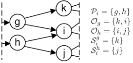
Figure 1: Illustration of predecessors, siblings and offsprings.

We make a simplifying yet plausible assumption that $\bigcup_{h\in{\cal P}_{i}}{\cal S}_{i}^{h}\cap{\cal P}_{i}=\emptyset$, i.e., no node can be both a sibling and a predecessor of any other node.

By our assumption on ${\cal G}$, $s$ is the only node without any predecessor while $w$ is the only node without any offspring. Since the pricing game to be studied can arise only if there are multiple relays competing for the traffic from their common predecessor, we assume in $\cal G$ that every node $i$ except $w$ has multiple relays in ${\cal O}_{i}$ unless ${\cal O}_{i}=\{w\}$.

Denote the rate of flow on $(i,j)\in{\cal E}$ by $f_{ij}$. A link flow vector $\boldsymbol{f}\triangleq(f_{ij})_{(i,j)\in{\cal E}}$ is a routing of the session traffic if it satisfies the flow conservation constraint: $\sum_{h\in{\cal O}_{s}}f_{sh}=R_{s}$, $\sum_{k\in{\cal P}_{w}}f_{kw}=R_{s}$, and for each relay $i$,

$$\sum_{h\in{\cal P}_{i}}f_{hi}=\sum_{j\in{\cal O}_{i}}f_{ij}\triangleq r_{i},$$

where $r_{i}$ denotes the incoming flow rate at $i$.

II-B Link Cost and Pricing Functions

Each link has a strictly increasing and strictly convex cost function $D_{ij}(f_{ij})$, which is private information to $i$ and $j$ only. For example, $D_{ij}(f_{ij})$ can represent the queuing delay incurred on $(i,j)$ with arrival rate $f_{ij}$, e.g. the average occupancy function $f_{ij}/(c_{ij}-f_{ij})$ of an M/M/1 queue with service rate $c_{ij}$. As another example, if the links are wireless, $D_{ij}(f_{ij})$ can measure the transmission power required for achieving rate $f_{ij}$. For example, if the link transmission rate $f_{ij}$ is determined by transmission power $P_{ij}$ as $f_{ij}=W\log(1+KP_{ij})$ for some constants $W,K>0$, then $P_{ij}=\frac{1}{K}\left(2^{f_{ij}/W}-1\right)\triangleq D_{ij}(f_{ij})$, which is strictly increasing and convex in $f_{ij}$. As suggested by the examples, the analytical framework presented above applies to both wireline and wireless networks.

For analytical purposes, we further assume that $D_{ij}(\cdot)$ is continuously differentiable with derivative $d_{ij}(\cdot)$. By previous assumptions, $d_{ij}(\cdot)$ is positive and strictly increasing. The socially optimal routing is the routing that minimizes the network cost $\sum_{(i,j)}D_{ij}(f_{ij})$. Because link costs are strictly convex, the socially optimal routing is uniquely characterized by the condition that every path from $s$ to $w$ with positive flow has the minimum marginal cost among all paths. For otherwise, one can reduce the total cost by shifting an infinitesimal amount of flow from a path with non-minimum marginal cost to a minimum-marginal-cost path.

We model the source and relays as selfish agents who must pay for the costs on their outgoing links. While the source has to send all its traffic out, it strives to do this with the minimum cost. On the other hand, a relay has an incentive to forward traffic for its predecessors only if it is adequately rewarded for its service in the form of payment by its predecessors. The amount of payment is determined as follows.

Suppose a node $h$ has incoming flow of rate $r_{h}>0$. Each $i\in{\cal O}_{h}$ announces a pricing function $P_{i}^{h}(\cdot)$ which specifies the payment $P_{i}^{h}(f_{hi})$ it demands should $h$ forward traffic of rate $f_{hi}$ to it. For analytical purposes, we assume that $P_{i}^{h}(t)$ is continuously differentiable with derivative $p_{i}^{h}(t)$. Note that $P_{i}^{h}(\cdot)$ provides $h$ a continuum of options, namely the rate-price pairs $(f_{hi},P_{i}^{h}(f_{hi}))$. After learning $(P_{i}^{h}(\cdot))_{i\in{\cal O}_{h}}$, $h$ decides on the allocation of $r_{h}$ and makes payments to its offsprings accordingly.

II-C Pricing Game

We assume every node is selfish and strategic. The source $s$ thus always allocates the total flow $R_{s}$ to the nodes in ${\cal O}_{s}$ so as to minimize its total cost, which includes the costs on its outgoing links and the payments to its offsprings. Specifically, given the pricing functions $P_{i}^{s}(\cdot)$ of $i\in{\cal O}_{s}$, the optimal allocation of $R_{s}$ from the perspective of $s$ is any

$$(f_{si}^{*})_{i\in{\cal O}_{s}}\in\mathop{\arg\min}_{(f_{si})\in{\cal F}_{s}(R_{s})}\sum_{i\in{\cal O}_{s}}D_{si}(f_{si})+P_{i}^{s}(f_{si}),$$ (1)

where ${\cal F}_{i}(r)$ is defined as $\{(f_{ik})_{k\in{\cal O}_{i}}\geq\boldsymbol{0}:\sum_{k}f_{ik}=r\}$.

A relay $i$ is a predecessor to some nodes, and is an offspring to some other nodes. As a predecessor, it acts just like $s$. That is, it allocates the total incoming flow in the most cost efficient way from its own perspective. Thus, the traffic allocation adopted by $i$ when it has incoming flow $r_{i}$ is any

$$(f_{ik}^{*})_{k\in{\cal O}_{i}}\in\mathop{\arg\min}_{(f_{ik})\in{\cal F}_{i}(r_{i})}\sum_{k\in{\cal O}_{i}}D_{ik}(f_{ik})+P_{k}^{i}(f_{ik}).$$ (2)

Denote the minimum value in (2) by $D_{i}(r_{i})$. Note that $D_{i}(r_{i})$ represents the minimum cost to $i$ for forwarding flow of rate $r_{i}$. It is easy to show that $D_{i}(\cdot)$ is continuous and increasing with piecewise continuous derivative denoted by $d_{i}(\cdot)$.

As an offspring, $i$ designs $P_{i}^{h}(\cdot)$ for every $h\in{\cal P}_{i}$ with the aim of maximizing its profit in competition with its siblings (discussed in depth later). It does this with the assumption that $h$ always allocates in the most cost efficient way, and that $r_{h}$ for each $h\in{\cal P}_{i}$ stays constant at the current value irrespective of its choice of $P_{i}^{h}(\cdot)$. While the first assumption is very reasonable, the second one requires some justification.

Theoretically, since $r_{h}$ of $h\in{\cal P}_{i}$ is the outcome of the optimal allocation by $h$’s predecessors, it in general cannot stay constant if $h$ changes its pricing functions. However, $h$’s pricing functions presumably are tied to $i$’s choice of $P_{i}^{h}(\cdot)$ as the total cost to $h$ is partly leveraged by the price charged by $i$. Once $h$ reacts to the change in $P_{i}^{h}(\cdot)$ by updating its own pricing functions, $r_{h}$ is inevitably adjusted by $h$’s predecessors. On the other hand, relays are usually too myopic to note this chain reaction since they have very limited knowledge of the network. Recall that we made a practical assumption that a relay is aware of only its predecessors, siblings and offsprings. As a result, it can at best predict the impact of its strategy on the traffic allocation by its predecessors, but not nodes further upstream. It is therefore reasonable for $i$ to consider only the competition with its siblings for the flow their common predecessors currently have.

We now formally define the (static) pricing game (PG) as having the following components:

• The set of players ${\cal I}={\cal N}\backslash\{s,w\}$: relays in ${\cal G}$.

• Strategy of player $i$: continuously differentiable pricing functions $P_{i}^{h}(\cdot)$ for all $h\in{\cal P}_{i}$.

• Payoff to player $i$: the profit made by servicing $(f_{hi}^{*})_{h\in{\cal P}_{i}}$:

  $$\sum_{h\in{\cal P}_{i}}P_{i}^{h}(f_{hi}^{*})-D_{i}\left(\sum_{h\in{\cal P}_{i}}f_{hi}^{*}\right),$$ (3)

  where the routing $(f_{ij}^{*})_{(i,j)\in{\cal E}}$ is most cost efficient from the perspective of every node, i.e., (1)-(2) hold for $s$ and every relay $i$ where $r_{i}=\sum_{h\in{\cal P}_{i}}f_{hi}^{*}$.

A pricing game is fully characterized by the tuple $({\cal G},(D_{ij}(\cdot)),R_{s})$. In the rest of the paper, we will study the outcome of the PG with myopic players as described above. The focus of our work is to investigate whether the PG has an equilibrium where no relay can increase its profit by unilaterally changing its pricing functions, and when an equilibrium exists, how the resulting routing compares to the socially optimal one.

II-D Best Response and Equilibrium

Each player $i$ in the PG is assumed to be myopic in the sense that it knows the pricing functions of all its competitors as well as its downstream nodes. Based on its local information $\boldsymbol{L}_{i}\triangleq((r_{h},(P_{j}^{h}(\cdot))_{j\in{\cal S}_{i}^{h}})_{h\in{\cal P}_{i}},(P_{k}^{i}(\cdot))_{k\in{\cal O}_{i}})$, player $i$ anticipates a payoff $\Gamma_{i}(\boldsymbol{P}_{i};\boldsymbol{L}_{i})$ when adopting $\boldsymbol{P}_{i}\triangleq(P_{i}^{h}(\cdot))_{h\in{\cal P}_{i}}$, where

$$\Gamma_{i}(\boldsymbol{P}_{i};\boldsymbol{L}_{i})\triangleq\sum_{h\in{\cal P}_{i}}P_{i}^{h}(f_{hi}^{*})-\sum_{k\in{\cal O}_{i}}\left[D_{ik}(f_{ik}^{*})+P_{k}^{i}(f_{ik}^{*})\right],$$

$(f_{hj}^{*})_{j\in{\cal O}_{h}}$ is the optimal allocation of $r_{h}$ by $h\in{\cal P}_{i}$ given $(P_{j}^{h}(\cdot))_{j\in{\cal O}_{h}}$, and $(f_{ik}^{*})_{k\in{\cal O}_{i}}$ is the optimal allocation of $r_{i}^{*}=\sum_{h\in{\cal P}_{i}}f_{hi}^{*}$ given $(P_{k}^{i}(\cdot))_{k\in{\cal O}_{i}}$.

Definition 1

A pricing function profile $(P_{i}^{h}(\cdot))_{h\in{\cal P}_{i}}$ is a best response to local information $\boldsymbol{L}_{i}$ if

$$\Gamma_{i}(\boldsymbol{P}_{i};\boldsymbol{L}_{i})=\max_{\boldsymbol{Q}_{i}\textrm{feasible}}\Gamma_{i}(\boldsymbol{Q}_{i};\boldsymbol{L}_{i}),$$

where $\boldsymbol{Q}_{i}=(Q_{i}^{h}(\cdot))_{h\in{\cal P}_{i}}$ is feasible if every component is a continuously differentiable function.

Denote the set of best responses to $\boldsymbol{L}_{i}$ by ${\cal B}_{i}(\boldsymbol{L}_{i})$. Before we proceed, we must prove that ${\cal B}_{i}(\boldsymbol{L}_{i})$ is non-empty.

Lemma 1

For any $\boldsymbol{L}_{i}$, the set ${\cal B}_{i}(\boldsymbol{L}_{i})$ is non-empty. Furthermore, $\boldsymbol{P}_{i}\in{\cal B}_{i}(\boldsymbol{L}_{i})$ if and only if for all $h\in{\cal P}_{i}$ and all $t\in[0,r_{h}]$,

$$B_{i}^{h}(t)\triangleq D_{hi}(t)+P_{i}^{h}(t)\geq B_{\hat{i}}^{h}(r_{h})-B_{\hat{i}}^{h}(r_{h}-t),$$ (4)

and

$$B_{i}^{h}(\tilde{f}_{hi})=B_{\hat{i}}^{h}(r_{h})-B_{\hat{i}}^{h}(r_{h}-\tilde{f}_{hi}),$$ (5)

where

$$B_{\hat{i}}^{h}(r)\triangleq\min_{\begin{subarray}{c}(f_{hj})\in{\cal F}_{h}(r)\\ f_{hi}=0\end{subarray}}\sum_{j\in{\cal S}_{i}^{h}}B_{j}^{h}(f_{hj})$$ (6)

and $(\tilde{f}_{hi})_{h\in{\cal P}_{i}}$ is a vector that maximizes

$$\bar{\Gamma}_{i}(\boldsymbol{f}_{i};\boldsymbol{L}_{i})\triangleq\sum_{h\in{\cal P}_{i}}\left[B_{\hat{i}}^{h}(r_{h})-B_{\hat{i}}^{h}(r_{h}-f_{hi})-D_{hi}(f_{hi})\right]-D_{i}\left(\sum_{h\in{\cal P}_{i}}f_{hi}\right)$$

over all the $\boldsymbol{f}_{i}=(f_{hi})$ such that $0\leq f_{hi}\leq r_{h}$ for all $h\in{\cal P}_{i}$.

Before giving the proof, we first provide some intuitive explanations for the lemma. The function $B_{i}^{h}(t)$ gives the total cost $h$ spends on routing traffic of rate $t$ to $i$. Since $D_{hi}(\cdot)$ is fixed and known to $i$, it is equivalent to treat $B_{i}^{h}(\cdot)$ as the pricing function $i$ uses to charge $h$. With this view, $h$ makes a lump-sum payment to $i$ determined by $B_{i}^{h}(\cdot)$, and lets $i$ pay for the cost $D_{hi}(\cdot)$ on link $(h,i)$. For convenience, from now on we assume each relay $i$ announces $B_{i}^{h}(\cdot)$ to $h\in{\cal P}_{i}$ and siblings $j\in{\cal S}_{i}^{h}$. By (6), $B_{\hat{i}}^{h}(r)$ represents the minimum cost $h$ can achieve by forwarding traffic of rate $r$ to offsprings other than $i$. It will become evident in the next proof that from $i$’s viewpoint, the competition from all $j\in{\cal S}_{i}^{h}$ can be aggregated into a virtual competitor $\hat{i}^{h}$ using pricing function $B_{\hat{i}}^{h}(\cdot)$. Thus, it is as if $i$ were competing with one relay $\hat{i}^{h}$ in each “market” $h\in{\cal P}_{i}$. The vector $(\tilde{f}_{hi})_{h\in{\cal P}_{i}}$ represents the “market shares” that jointly yield the maximum (anticipated) profit to $i$. Pricing functions $B_{i}^{h}(\cdot)$ which satisfy the conditions in Lemma 1 induce $h\in{\cal P}_{i}$ to allocate the ideal “market share” $\tilde{f}_{hi}$ to $i$ and give $i$ the maximum profit. This is because (5) implies that allocating $\tilde{f}_{hi}$ to $i$ and the rest to other relays yields the same cost to $h$ as allocating all the traffic to other relays. So conditions (4) and (5) combined imply that no other allocation costs less than the above two schemes.

Proof of Lemma 1: First notice that for fixed $\boldsymbol{L}_{i}$, the profit of $i$ when it adopts $(B_{i}^{h}(\cdot))_{h\in{\cal P}_{i}}$ is upper bounded as follows:

$$\Gamma_{i}((B_{i}^{h}(\cdot));\boldsymbol{L}_{i}) = \sum_{h\in{\cal P}_{i}}\left[B_{i}^{h}(f_{hi})-D_{hi}(f_{hi})\right]-D_{i}\left(\sum_{h\in{\cal P}_{i}}f_{hi}\right)$$

$$\leq \sum_{h\in{\cal P}_{i}}\left[B_{\hat{i}}^{h}(r_{h})-B_{\hat{i}}^{h}(r_{h}-f_{hi})-D_{hi}(f_{hi})\right]-D_{i}\left(\sum_{h\in{\cal P}_{i}}f_{hi}\right)$$

$$= \bar{\Gamma}_{i}(\boldsymbol{f}_{i};\boldsymbol{L}_{i})\leq\bar{\Gamma}_{i}(\boldsymbol{\tilde{f}_{i}};\boldsymbol{L}_{i}),$$

where $\boldsymbol{f}_{i}\triangleq(f_{hi})_{h\in{\cal P}_{i}}$ is the optimal amount of traffic allocated to $i$ when $i$ uses $(B_{i}^{h}(\cdot))$. The first inequality holds because for every $h\in{\cal P}_{i}$, $B_{i}^{h}(f_{hi})\leq B_{\hat{i}}^{h}(r_{h})-B_{\hat{i}}^{h}(r_{h}-f_{hi})$. For otherwise, $h$ would find the cost of allocating $r_{h}$ exclusively to all $j\in{\cal S}_{i}^{h}$ ($B_{\hat{i}}^{h}(r_{h})$) strictly less than the cost of allocating $f_{hi}$ to $i$ and $r_{h}-f_{hi}$ to $j\in{\cal S}_{i}^{h}$ ($B_{i}^{h}(f_{hi})+B_{\hat{i}}^{h}(r_{h}-f_{hi})$), a contradiction. The second inequality follows from the definition of $\tilde{{\boldsymbol{f}}_{i}}$.

Notice that the upper bound $\bar{\Gamma}_{i}(\boldsymbol{\tilde{f}_{i}};\boldsymbol{L}_{i})$ is independent of $(B_{i}^{h}(\cdot))$. It is tight if and only if both inequalities hold with equality. To make the second inequality tight, it is necessary and sufficient to have the traffic allocation $\boldsymbol{f}_{i}$ induced by $(B_{i}^{h}(\cdot))$ equal to $\boldsymbol{\tilde{f}_{i}}$. Given that, the first inequality is tight if (4)-(5) hold, since they guarantee that allocating $\tilde{f}_{hi}$ to $i$ and $r_{h}-\tilde{f}_{hi}$ to $j\in{\cal S}_{i}^{h}$ is in $h$’s best interest. They are also necessary because (5) is prerequisite for the first inequality to be tight, and consequently (4) cannot be violated either. For example, if for some $h\in{\cal P}_{i}$ and some $t\in[0,r_{h}]$, $B_{i}^{h}(t)<B_{\hat{i}}^{h}(r_{h})-B_{\hat{i}}^{h}(r_{h}-t)$. Then allocating $t$ to $i$ and $r_{h}-t$ to $j\in{\cal S}_{i}^{h}$ would incur strictly less cost to $h$ than $B_{\hat{i}}^{h}(r_{h})=B_{i}^{h}(t)(\tilde{f}_{hi})+B_{\hat{i}}^{h}(r_{h}-\tilde{f}_{hi})$. Thus, $h$ would not have allocated $\tilde{f}_{hi}$ to $i$, which is a contradiction. ∎

Note that best response $(B_{i}^{h}(\cdot))$ always exists because, for instance, $B_{i}^{h}(t)=B_{\hat{i}}^{h}(r_{h})-B_{\hat{i}}^{h}(r_{h}-t)$ for $t\in[0,r_{h}]$ satisfies (4)-(5). The (pure-strategy) Nash equilibria are defined as the fixed points of the best response mapping.

Definition 2

Pricing function profiles $\boldsymbol{P}_{i},i\in{\cal I}$ constitute an equilibrium if for all $i\in{\cal I}$, $\boldsymbol{P}_{i}\in{\cal B}_{i}(\boldsymbol{L}_{i})$ where the incoming flow vector $(r_{h})_{h\in{\cal P}_{i}}$ contained in $\boldsymbol{L}_{i}$ results from the routing $(f_{ij}^{*})_{(i,j)\in{\cal E}}$ that is most cost efficient from the perspective of every individual node, i.e., (1)-(2) hold for $s$ and all $i\in{\cal I}$,

$$r_{h}=\sum_{g\in{\cal P}_{h}}f_{gh}^{*},\quad\textrm{if}~{}h\neq s$$

and $r_{h}=R_{s}$ if $h=s$.

It is easy to see that if $(\boldsymbol{P}_{i})_{i\in{\cal I}}$ constitutes an equilibrium, $\Gamma_{i}(\boldsymbol{P}_{i};\boldsymbol{L}_{i})$ must coincide with the actual payoff of $i$.

Definition 3

An equilibrium $(\boldsymbol{P}_{i})_{i\in{\cal I}}$ is efficient if it induces the socially optimal routing. In this case, $(\boldsymbol{P}_{i})_{i\in{\cal I}}$ is said to induce the social optimum.

Before proving the existence of equilibria and analyzing their efficiency in the general setting, we first study pricing games under some simple network topologies. The analysis of these games not only provide valuable insight into the general problem but also have significant implications in their own right.

III Equilibria in Oligopoly

The simplest topologies within our framework are those including a single layer of relays, e.g. the one in Figure 2.

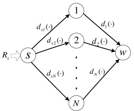
Figure 2: Oligopoly with N relays.

Here, $N$ relays each have a direct link from $s$ and a direct link to $w$. They compete for the total flow $R_{s}$ by advertising their pricing functions $\beta_{i}(\cdot)=d_{si}(\cdot)+p_{i}(\cdot),i=1,\cdots,N$. From now on, we will more often refer to the derivatives $d_{ij}(\cdot)$ and $p_{i}(\cdot)$ as link cost and pricing functions, since they appear to be more convenient for marginal cost analysis at equilibria. Also we will use simplified notation whenever appropriate, e.g. the superscript is omitted from $p_{i}(\cdot),\beta_{i}(\cdot)$ as $s$ is the only predecessor to every relay. We refer to a pricing game under such a topology as an oligopoly. Define $\lambda_{i}(t)\triangleq d_{si}(t)+d_{i}(t)$. An oligopoly PG is fully characterized by the tuple $(N,(\lambda_{i}(\cdot))_{i=1}^{N},R_{s})$.

Because all $\lambda_{i}(\cdot)$ are strictly increasing, the socially optimal routing $(r_{i}^{*})_{i=1}^{N}$ is unique and is given by

$$\lambda_{i}(r_{i}^{*})=\min_{j=1,\cdots,N}\lambda_{j}(r_{j}^{*})$$

if $r_{i}^{*}>0$.

We now analyze the routing established by the oligopoly PG. Given $(\beta_{i}(\cdot))_{i\in{\cal O}_{s}}$, the self-interest of $s$ leads it to adopt the most cost efficient routing $(f_{si}^{*})_{i=1}^{N}$ such that

$$\beta_{i}(f_{si}^{*})=\min_{j=1,\cdots,N}\beta_{j}(f_{sj}^{*})$$ (7)

whenever $f_{si}^{*}>0$. Whether $(f_{si}^{*})=(r_{i}^{*})$ or not depends on how $(\beta_{i}(\cdot))$ are chosen by the individual relays.

III-A Best Response and Existence of Equilibria

We apply Lemma 1 to the oligopoly PG. Here,

$$B_{i}(t)=\int_{0}^{t}\beta_{i}(r)~{}dr,$$

$$B_{\hat{i}}(t)=\min_{\sum_{j\neq i}f_{sj}=t}\sum_{j\neq i}\int_{0}^{f_{sj}}\beta_{j}(r)~{}dr.$$

It is easy to show that $B_{\hat{i}}(t)$ is continuous and increasing. Its derivative, denoted by $\beta_{\hat{i}}(t)$, is in general piecewise continuous. For $t\in(0,R_{s})$, let the left and right limits of $\beta_{\hat{i}}(t)$ be denoted by $\beta_{\hat{i}}(t)^{-}$ and $\beta_{\hat{i}}(t)^{+}$. By Lemma 1, the best response of $i$ given $\beta_{\hat{i}}(\cdot)$ can be simply characterized by

$$\int_{0}^{t}\beta_{i}(r)~{}dr\left\{\begin{array}[]{ll}\geq\int_{0}^{t}\beta_{\hat{i}}(R_{s}-r)~{}dr,&0\leq t\leq R_{s}\\ =\int_{0}^{t}\beta_{\hat{i}}(R_{s}-r)~{}dr,&t=f_{i}^{*},\end{array}\right.$$ (8)

where

$$f_{i}^{*}\in\mathop{\arg\max}_{0\leq f_{i}\leq R_{s}}\int_{0}^{f_{i}}\beta_{\hat{i}}(R_{s}-r)-\lambda_{i}(r)~{}dr.$$ (9)

To gain an intuitive idea of the above conditions, suppose $\beta_{\hat{i}}(R_{s}-r)$ and $\lambda_{i}(r)$ are given by the dashed and solid curves in Figure 3. A typical best response $\beta_{i}(r)$ is shown as the dotted curve.

Figure 3: Typical best response curve in oligopoly.

In particular, one can let $\beta_{i}(r)$ coincide with $\beta_{\hat{i}}(R_{s}-r)$ on $[0,f_{i}^{*}]$ and let $\beta_{i}(r)\geq\beta_{\hat{i}}(R_{s}-r)$ on $(f_{i}^{*},R_{s}]$. Such a best response will be referred to as a replicating response. As we will show, oligopoly equilibria induced by replicating responses are always efficient while equilibria induced by other best responses are not necessarily efficient.

III-B Efficient Equilibria

Theorem 1

The socially optimal routing of an oligopoly can always be induced by an equilibrium.

Proof: We prove the theorem by constructing an equilibrium that induces the socially optimal routing $(r_{i}^{*})$. Define $\lambda^{*}\triangleq\min_{j=1,\cdots,N}\lambda_{j}(r_{j}^{*})$. Let $\beta_{i}(r)\equiv\lambda^{*}$ for all $i$. Then $\beta_{i}(r)=\beta_{\hat{i}}(R_{s}-r)=\lambda^{*}$ is a best response for all $i$ with $f_{i}^{*}=r_{i}^{*}$. Thus, $(\beta_{i}(\cdot))$ constitutes an equilibrium which results in the routing $(r_{i}^{*})$. ∎

Because the socially optimal routing always exists, we can conclude that there always exists an efficient equilibrium for any oligopoly pricing game.

Although we used constant $(\beta_{i}(\cdot))$ (or linear pricing functions $(B_{i}(\cdot))$) to construct an efficient equilibrium in the proof, efficient equilibria can be established by nonlinear pricing functions as well. For instance, Figure 4 depicts an equilibrium in a duopoly PG where the two relays adopt $\beta_{1}(\cdot),\beta_{2}(\cdot)$ of a more general shape. Notice that in a duopoly, $\beta_{\hat{1}}(t)=\beta_{2}(t)$ and $\beta_{\hat{2}}(t)=\beta_{1}(t)$.

Figure 4: General (focal) equilibrium in duopoly.

To derive a simple criterion for checking the efficiency of an equilibrium, we need to make the following distinction. A routing $(f_{i})_{i=1}^{N}$ is said to be monopolistic if $f_{m}=R_{s}$ for some relay $m$ and $f_{j}=0$ for all $j\neq m$. In this case, $m$ is called the dominant relay. An equilibrium is monopolistic if it induces a monopolistic routing. A routing is said to be competitive if there are at least two relays $i,j$ such that $f_{i}>0,f_{j}>0$. An equilibrium is competitive if it induces a competitive routing.

Theorem 2

If an oligopoly equilibrium is competitive, it must be efficient.

We will need the next lemma to prove Theorem 2.

Lemma 2

At an oligopoly equilibrium $(\beta_{i}(\cdot))$ which induces routing $(f_{i}^{*})$, if $0<f_{i}^{*}\leq R_{s}$, then for all $j\neq i$,

$$\beta_{\hat{i}}(R_{s}-f_{i}^{*})^{+}\leq\beta_{j}(f_{j}^{*}).$$

If $0\leq f_{i}^{*}<R_{s}$, then for all $j\neq i$ such that $f_{j}^{*}>0$,

$$\beta_{\hat{i}}(R_{s}-f_{i}^{*})^{-}\geq\beta_{j}(f_{j}^{*}).$$

Proof: By definition, if $t<R_{s}$, $\beta_{\hat{i}}(t)^{+}=\lim_{\Delta\to 0^{+}}(B_{\hat{i}}(t+\Delta)-B_{\hat{i}}(t))/\Delta$. Therefore when $f_{i}^{*}>0$,

$$\beta_{\hat{i}}(R_{s}-f_{i}^{*})^{+} = \lim_{\Delta\to 0^{+}}\frac{1}{\Delta}\left\{B_{\hat{i}}(R_{s}-f_{i}^{*}+\Delta)-B_{\hat{i}}(R_{s}-f_{i}^{*})\right\}$$

$$\stackrel{{\scriptstyle(a)}}{{=}} \lim_{\Delta\to 0^{+}}\frac{1}{\Delta}\left\{\min_{\sum_{j\neq i}f_{j}=R_{s}-f_{i}^{*}+\Delta}\sum_{j\neq i}\int_{0}^{f_{j}}\beta_{j}(r)~{}dr-\sum_{j\neq i}\int_{0}^{f_{j}^{*}}\beta_{j}(r)~{}dr\right\}$$

$$\stackrel{{\scriptstyle(b)}}{{\leq}} \lim_{\Delta\to 0^{+}}\frac{1}{\Delta}\left\{\int_{0}^{f_{k}^{*}+\Delta}\beta_{k}(r)~{}dr+\sum_{j\neq i,k}\int_{0}^{f_{j}^{*}}\beta_{j}(r)~{}dr-\sum_{j\neq i}\int_{0}^{f_{j}^{*}}\beta_{j}(r)~{}dr\right\}$$

$$= \lim_{\Delta\to 0^{+}}\frac{1}{\Delta}\int_{f_{k}^{*}}^{f_{k}^{*}+\Delta}\beta_{k}(r)~{}dr=\beta_{k}(f_{k}^{*}).$$

Here, equation (a) follows from the fact that $(f_{j}^{*})_{j=1}^{N}$ is the equilibrium routing of $R_{s}$ induced by $(\beta_{j}(\cdot))_{j=1}^{N}$. Inequality (b) is obtained by substituting the minimum-cost routing of $R_{s}-f_{i}^{*}+\Delta$ by an arbitrary routing, namely $f_{k}^{*}+\Delta$ allocated to $k$ and $f_{j}^{*}$ to each $j\neq i,k$. The second inequality in the lemma can be proved in a similar manner.∎

Proof of Theorem 2: Let $(f_{i}^{*})$ be the routing induced by a competitive equilibrium $(\beta_{i}(\cdot))$. Let $m,n$ be any two relays such that $f_{m}^{*}>0,f_{n}^{*}>0$. It is enough to show that $\lambda_{m}(f_{m}^{*})=\lambda_{n}(f_{n}^{*})$ and that $\lambda_{m}(f_{m}^{*})\leq\lambda_{j}(f_{j}^{*})$ for any $j$ with $f_{j}^{*}=0$. By (7), $\beta_{m}(f_{m}^{*})=\beta_{n}(f_{n}^{*})$. The best response condition (9) implies that $\beta_{\hat{m}}(R_{s}-f_{m}^{*})^{-}\leq\lambda_{m}(f_{m}^{*})\leq\beta_{\hat{m}}(R_{s}-f_{m}^{*})^{+}$. By Lemma 2, $\beta_{n}(f_{n}^{*})\leq\beta_{\hat{m}}(R_{s}-f_{m}^{*})^{-}$ and $\beta_{\hat{m}}(R_{s}-f_{m}^{*})^{+}\leq\beta_{n}(f_{n}^{*})$. In conclusion, $\beta_{n}(f_{n}^{*})=\lambda_{m}(f_{m}^{*})$. By symmetry, we can show that $\beta_{m}(f_{m}^{*})=\lambda_{n}(f_{n}^{*})$. Therefore, $\lambda_{m}(f_{m}^{*})=\lambda_{n}(f_{n}^{*})$. Now suppose $f_{j}^{*}=0$. By (9) and Lemma 2, $\lambda_{j}(0)\geq\beta_{\hat{j}}(R_{s})^{-}\geq\beta_{n}(f_{n}^{*})=\lambda_{m}(f_{m}^{*})$. So the proof is complete. ∎

III-C Inefficient Equilibria

Theorem 2 does not rule out the possibility of inefficient equilibria. In fact, an equilibrium may be inefficient if it is monopolistic. For example, the socially optimal routing of the duopoly PG represented by Figure 5 is $(r_{1}^{*},R_{s}-r_{1}^{*})$ whereas the equilibrium depicted leads to a monopolistic routing $(R_{s},0)$.

Figure 5: Inefficient equilibrium in duopoly.

In this example, relay $2$ adopts a pricing function $\beta_{2}(\cdot)$ such that $\int_{0}^{R_{s}}\beta_{2}(r)~{}dr=\int_{0}^{R_{s}}\lambda_{2}(r)~{}dr$ and $\beta_{2}(R_{s}-r)>\lambda_{1}(r)$ for all $r\in[0,R_{s}]$. Given such a $\beta_{2}(\cdot)$, relay $1$ would want to acquire all the flow (cf. (9)) by using $\beta_{1}(\cdot)$ such that $\int_{0}^{t}\beta_{1}(R_{s}-r)~{}dr<\int_{0}^{t}\lambda_{2}(r)~{}dr$ and $\int_{0}^{t}\beta_{1}(r)~{}dr>\int_{0}^{t}\beta_{2}(R_{s}-r)~{}dr$ for all $t\in(0,R_{s})$ and $\int_{0}^{R_{s}}\beta_{1}(R_{s}-r)~{}dr=\int_{0}^{R_{s}}\lambda_{2}(r)~{}dr=\int_{0}^{R_{s}}\beta_{2}(r)~{}dr$. Thus, it satisfies (8) and leaves relay $2$ no incentive to acquire any traffic. So the monopolistic equilibrium holds.

In general, monopolistic equilibria in an oligopoly PG have the following property.

Theorem 3

If an oligopoly equilibrium is monopolistic with dominant relay $m$, we must have

$$\int_{0}^{R_{s}}\lambda_{m}(r)~{}dr\leq\int_{0}^{R_{s}}\lambda_{j}(r)~{}dr$$

for any other relay $j$.

Proof: Consider any $j$ with $f_{j}^{*}=0$ in a monopolistic equilibrium. The condition (9) implies that

$$\int_{0}^{R_{s}}\lambda_{j}(r)~{}dr\geq\int_{0}^{R_{s}}\beta_{\hat{j}}(R_{s}-r)~{}dr.$$

On the other hand,

$$\int_{0}^{R_{s}}\beta_{\hat{j}}(R_{s}-r)~{}dr=\int_{0}^{R_{s}}\beta_{\hat{j}}(r)~{}dr=\int_{0}^{R_{s}}\beta_{m}(r)~{}dr,$$

since from the perspective of $s$, the optimal allocation of $R_{s}$ to all the relays except $j$ still assigns all the traffic to $m$. It follows from $m$’s best response conditions (8)-(9) that

$$\int_{0}^{R_{s}}\beta_{m}(r)~{}dr=\int_{0}^{R_{s}}\beta_{\hat{m}}(R_{s}-r)~{}dr\geq\int_{0}^{R_{s}}\lambda_{m}(r)~{}dr.$$

Thus the proof is complete. ∎

The next conclusion easily follows from Theorem 3.

Corollary 1

If the socially optimal routing of an oligopoly is monopolistic, then every equilibrium of the oligopoly is monopolistic and efficient.

Proof: It can deduced from the uniqueness of the socially optimal routing and Theorem 2 that every equilibrium of such an oligopoly must be monopolistic. By Theorem 3, the dominant relay $m$ of such an equilibrium has the minimum $\int_{0}^{R_{s}}\lambda_{m}(r)~{}dr$ among all relays. But such an $m$ must be the dominant relay in the socially optimal routing. ∎

It is shown next that there always exists a monopolistic equilibrium in an oligopoly. Thus, we have the following conclusion.

Corollary 2

If the socially optimal routing of an oligopoly is competitive, then there exists an inefficient (monopolistic) equilibrium.

Proof: We need only show that there exists a monopolistic equilibrium in such an oligopoly. Let all $\beta_{j}(\cdot)$ be the same strictly decreasing function $\beta(\cdot)$ such that $\int_{0}^{t}\beta(R_{s}-r)dr\leq\int_{0}^{t}\lambda_{j}(r)dr$ for all $j$ and $t\in[0,R_{s})$ but $\int_{0}^{R_{s}}\beta(R_{s}-r)dr=\int_{0}^{R_{s}}\lambda_{m}(r)dr$ where $m\in\arg\min_{j}\int_{0}^{R_{s}}\lambda_{j}(r)dr$. Since $\beta(\cdot)$ is strictly decreasing, $\beta_{\hat{j}}(r)=\beta(r)$ for all $j$. By construction, $f_{j}^{*}=0$ is an ideal flow to $j\neq m$ (cf. (9)) whereas $\beta_{m}(\cdot)=\beta(\cdot)$ and $f_{m}^{*}=R_{s}$ jointly satisfy $m$’s best response conditions (8)-(9). So the monopolistic equilibrium is established. ∎

When an oligopoly has inefficient equilibria, it is of interest to compare the worst-case network cost under an inefficient equilibrium to the optimal cost.

III-D Price of Anarchy

The price of anarchy, as a measure of loss of social efficiency due to selfish behavior of individual agents, was studied in the literature on selfish routing [8, 9]. In this work, the price of anarchy of a general PG is defined as follows.

Definition 4

The price of anarchy $\rho({\cal G},(D_{ij}(\cdot)),R_{s})$ of a pricing game $({\cal G},(D_{ij}(\cdot)),R_{s})$ is the ratio of the maximum cost at an equilibrium to the socially optimal cost, i.e.,

$$\rho({\cal G},(D_{ij}(\cdot)),R_{s})\triangleq\frac{\max_{(f_{ij})\in{\cal F}^{E}}\sum_{(i,j)\in{\cal E}}D_{ij}(f_{ij})}{\sum_{(i,j)\in{\cal E}}D_{ij}(f_{ij}^{*})},$$

where ${\cal F}^{E}$ is the collection of all routings that can be induced by an equilibrium of $({\cal G},(D_{ij}(\cdot)),R_{s})$ and $(f_{ij}^{*})_{(i,j)\in{\cal E}}$ is the socially optimal routing of the game.

In this section, we study the price of anarchy specifically for oligopolies. As we will show, $\rho(N,(\lambda_{i}(\cdot)),R_{s})$ is equal to $N$ when marginal cost functions are concave, e.g. when cost functions are quadratic. However, the price of anarchy can be arbitrarily large when when marginal cost functions are convex, as is the case for the cost functions discussed in Section II-B.

Theorem 4

If the cost derivatives $(\lambda_{i}(\cdot))$ are concave, $\rho(N,(\lambda_{i}(\cdot)),R_{s})$ of an oligopoly pricing game is upper bounded by the number of relays $N$. The upper bound is achieved when the cost derivatives are linear.

Proof: Let the socially optimal routing be $(r_{i}^{*})_{i=1}^{N}=(\alpha_{i}R_{s})_{i=1}^{N}$ where the coefficients $(\alpha_{i})$ are nonnegative and sum to one. The optimal cost then is

$$D^{*}=\sum_{i=1}^{N}\int_{0}^{\alpha_{i}R_{s}}\lambda_{i}(r)~{}dr.$$

Since $\lambda_{i}(r)$ is concave, it can be shown that $\int_{0}^{\alpha_{i}R_{s}}\lambda_{i}(r)dr\geq\alpha_{i}^{2}\int_{0}^{R_{s}}\lambda_{i}(r)dr$ where equality holds when $\lambda_{i}(r)$ is linear. Therefore, $D^{*}$ is lower bounded as

$$D^{*}\geq\sum_{i=1}^{N}\alpha_{i}^{2}\int_{0}^{R_{s}}\lambda_{i}(r)~{}dr.$$

Recall that inefficient equilibria in an oligopoly are monopolistic such that the dominant relay $m$ satisfies Theorem 3. The price of anarchy, which is the ratio of the cost at any monopolistic equilibrium (ME) to $D^{*}$, is upper bounded as

$$\frac{D^{ME}}{D^{*}}\stackrel{{\scriptstyle(a)}}{{\leq}}\frac{\int_{0}^{R_{s}}\lambda_{m}(r)~{}dr}{\sum_{i=1}^{N}\alpha_{i}^{2}\int_{0}^{R_{s}}\lambda_{i}(r)~{}dr}\stackrel{{\scriptstyle(b)}}{{\leq}}\frac{\int_{0}^{R_{s}}\lambda_{m}(r)~{}dr}{\sum_{i=1}^{N}\alpha_{i}^{2}\int_{0}^{R_{s}}\lambda_{m}(r)~{}dr}=\frac{1}{\sum_{i=1}^{N}\alpha_{i}^{2}}\stackrel{{\scriptstyle(c)}}{{\leq}}N.$$

Next we specify the condition under which the upper bound is achieved. Notice that (a) holds with equality if and only if $\int_{0}^{\alpha_{i}R_{s}}\lambda_{i}(r)dr=\alpha_{i}^{2}\int_{0}^{R_{s}}\lambda_{i}(r)dr$ for all $i$. This requires each $\lambda_{i}(r)$ to be a linear function. Inequality (b) is tight when $\int_{0}^{R_{s}}\lambda_{i}(r)dr=\int_{0}^{R_{s}}\lambda_{m}(r)dr$ for every $i\neq m$. Hence, all the relays must have the same linear $\lambda_{i}(r)$. Thus, $(r_{i}^{*})$ must be the uniform, hence competitive, allocation, i.e., $\alpha_{i}=1/N$ for all $i$. This is exactly what is needed to make (c) tight.

Now it remains to find the pricing functions which can induce the monopolistic equilibrium attaining the upper bound. Let $\beta_{i}(r)=\lambda(R_{s}-r)\triangleq\beta(r)$ for every $i$. Since $\beta_{i}(r)$ is strictly decreasing for every $i$, $\beta_{\hat{i}}(r)=\beta(r)=\lambda(R_{s}-r)$. Since $\beta_{\hat{i}}(R_{s}-r)=\lambda(r)$, every relay is indifferent to having any amount of flow. Thus, the monopolistic equilibrium can be sustained. ∎

Unlike the selfish routing games considered in [8, 9], for which the price of anarchy is independent of the topology [18], Theorem 4 indicates that $\rho(N,(\lambda_{i}(\cdot)),R_{s})$ of an oligopoly PG explicitly depends on topology through $N$. Such a conclusion implies that the more intensive (larger $N$) the competition is, the more inefficient the market becomes if it is monopolized. The situation is even worse if the relays in an oligopoly have convex $\lambda_{i}(\cdot)$. In this case, the price of anarchy can be arbitrarily large.

Theorem 5

For a fixed number $N\geq 2$ of relays and for any $M>0$, there exists an oligopoly $(N,(\lambda_{i}(\cdot))_{i=1}^{N},R_{s})$ with convex $(\lambda_{i}(\cdot))$ such that $\rho(N,(\lambda_{i}(\cdot)),R_{s})\geq M$.

Sketch of Proof: We can construct an oligopoly with $N$ relays such that the socially optimal routing is competitive. By Corollary 2, inefficient monopolistic equilibria exist. However, within the class of convex functions, $\lambda_{m}(\cdot)$ of the dominant relay $m$ can be designed so that $\int_{0}^{R_{s}}\lambda_{m}(\cdot)\geq MD^{*}$, where $D^{*}$ is the optimal cost. ∎

III-E Focal Equilibria

Although possible, inefficient equilibria in an oligopoly are very unlikely to happen. The example in Figure 5 represents a highly pathological situation. Such an equilibrium is reached only if the subtle relationships between $\beta_{2}(\cdot)$ and $\lambda_{1}(\cdot)$ and between $\beta_{1}(\cdot)$ and $\lambda_{2}(\cdot)$ are satisfied. These relationships, however, can be established only by coincidence, since relay $2$ cannot observe $\lambda_{1}(\cdot)$ and relay $1$ cannot observe $\lambda_{2}(\cdot)$. In a general PG, it is arguably most rational for a relay to use a replicating response as described in Section III-A.

Definition 5

A focal equilibrium of a general pricing game is an equilibrium where every relay $i$ adopts the replicating response to its local information $\boldsymbol{L}_{i}=((r_{h},(B_{j}^{h}(\cdot))_{j\in{\cal S}_{i}^{h}})_{h\in{\cal P}_{i}},(B_{k}^{i}(\cdot))_{k\in{\cal O}_{i}})$, i.e., for all $h\in{\cal P}_{i}$,

$$B_{i}^{h}(t)\left\{\begin{array}[]{ll}=B_{\hat{i}}^{h}(r_{h})-B_{\hat{i}}^{h}(r_{h}-t),&t\in[0,f_{hi}^{*}]\\ \geq B_{\hat{i}}^{h}(r_{h})-B_{\hat{i}}^{h}(r_{h}-t),&t\in(f_{hi}^{*},r_{h}]\end{array}\right.,$$ (10)

where $(B_{\hat{i}}^{h}(\cdot),f_{hi}^{*})_{h\in{\cal P}_{i}}$ are as specified in Lemma 1.

In this section, we investigate focal equilibria in oligopolies. Such equilibria are not only reasonable for implementation, but also, more importantly, always efficient. The next theorem establishes the existence of focal equilibria in an oligopoly.

Theorem 6

The socially optimal routing of an oligopoly is always induced by a focal equilibrium.

Proof: Note that the equilibrium constructed in the proof of Theorem 1 is a focal equilibrium. ∎

Figure 4 illustrates a focal equilibrium in a duopoly induced by nonlinear pricing functions $B_{1}(\cdot),B_{2}(\cdot)$. The linear pricing equilibrium used in the proof is a special case of Figure 4 such that the curves of $\beta_{1}(r)$ and $\beta_{2}(r)$ are the same horizontal line that passes the point where $\lambda_{1}(r)$ and $\lambda_{2}(R_{s}-r)$ intersect. Notice that the focal equilibria encompassed by the above example have a common property. That is, the curves $\beta_{i}(\cdot)$ and $\lambda_{i}(\cdot)$ of all $i$ intersect at the point that corresponds to the social optimum. The next theorem states that such a phenomenon is no coincidence.

Theorem 7

Every focal equilibrium of an oligopoly is efficient.

Proof: In light of Theorem 2, we only need to show that any monopolistic focal equilibrium is efficient. Let $(\beta_{i}(\cdot))$ be the pricing functions that induce such an equilibrium where $m$ is the dominant relay. By the best response condition (9) and the fact that $\beta_{m}(\cdot)$ is a replicating response to $\beta_{\hat{m}}(\cdot)$, at $f_{m}^{*}=R_{s}$,

$$\lambda_{m}(R_{s})\leq\beta_{\hat{m}}(0)^{+}=\beta_{m}(R_{s})^{-}.$$

Applying (9) and Lemma 2 to any $j\neq m$, we have

$$\lambda_{j}(0)\geq\beta_{\hat{j}}(R_{s})^{-}\geq\beta_{m}(R_{s})^{-}.$$

Therefore, $\lambda_{m}(R_{s})\leq\lambda_{j}(0)$ for any $j\neq m$, which implies that the monopolistic routing is efficient. ∎

To summarize, as the most reasonable outcomes of a pricing game, focal equilibria always exist and are always efficient in oligopolies. We have yet to find out whether these properties hold in general PGs. In the remainder of the paper, we focus on the class of focal equilibria when we study pricing games in multi-hop networks. For brevity, we will drop the qualifier “focal” henceforth.

IV Equilibria in General Pricing Game

In this section, we consider a general multi-hop relay network with one source-destination pair as described in Section II. As in Section III, we assume that in every local competition, a relay $i$ declares $\beta_{i}^{h}(\cdot)=p_{i}^{h}(\cdot)+d_{hi}(\cdot)$ to an $h\in{\cal P}_{i}$ and all $j\in{\cal S}_{i}^{h}$.

Notice that if $h\in{\cal P}_{i}$ has $r_{h}=0$, then technically any $\beta_{i}^{h}(\cdot)$ is a best response since the local competition involving $i$ and $j\in{\cal S}_{i}^{h}$ is vacuous. To prevent absurd equilibria resulting from such arbitrary pricing, however, we assume that $i$ uses honest pricing $\beta_{i}^{h}(t)=d_{hi}(t)+d_{i}(t+\sum_{h^{\prime}\in{\cal P}_{i}\backslash h}f_{h^{\prime}i}^{*})$ when $r_{h}=0$. Here, $f_{h^{\prime}i}^{*}$ is the flow $i$ intends to acquire from $h^{\prime}\in{\cal P}_{i}\backslash h$, $d_{i}(t+\sum_{h^{\prime}\in{\cal P}_{i}\backslash h}f_{h^{\prime}i}^{*})$ is the derivative of the minimum cost incurred by $i$ in forwarding traffic to its offsprings. Thus, $\beta_{i}^{h}(t)$ exactly matches the actual cost of $i$ for forwarding flow from $h$. Honest pricing, though restrictive, is in line with $i$’s self interest. Being honest with its own cost, $i$ maximally alleviates the burden of $h$, whose cost is partly leveraged by $\beta_{i}^{h}(\cdot)$. Therefore, honest pricing can be seen as the best effort by $i$ to help improve the competitiveness of $h$, in the hope of earning profit from $h$ should $h$ later receive positive $r_{h}$ from its predecessors.

We will frequently use the following terms. A path is a concatenation of links from $s$ to $w$, while a sub-path is a contiguous segment of a path from a relay to $w$. Given a routing $(f_{ij})_{(i,j)\in{\cal E}}$, a path/sub-path is said to have positive flow if $f_{mn}>0$ for every $(m,n)$ in that path/sub-path. Otherwise, the path/sub-path is said to have zero flow. The marginal cost on a path/sub-path is the sum of $d_{mn}(f_{mn})$ over all $(m,n)$ on that path/sub-path.

Theorem 8

The socially optimal routing of a general PG can be induced by an equilibrium.

Due to its length, the proof of the theorem is deferred to Appendix -A.

IV-A Inefficient Equilibria and Price of Anarchy

Unlike the oligopoly case, in a general PG, not all focal equilibria are efficient. The inefficiency of an equilibrium in general PG’s is caused not only by the manipulative behavior of dominant relays but also by the myopia of nodes. We illustrate this point by the game depicted in Figure 6.

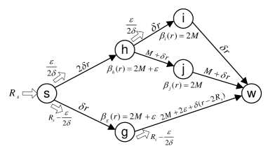
Figure 6: Arbitrarily bad equilibrium of a general PG.

The derivative of link cost functions are marked above each link, e.g. $d_{gw}(r)=2M+2\varepsilon+\delta(r-2R_{s})$, where $M$, $\varepsilon$ and $\delta$ are positive constants such that $M\gg\varepsilon R_{s}$ and $M\gg\delta R_{s}$. The pricing function of each node is marked above the node. There are three paths from $s$ to $w$, of which $(s,h,i,w)$ has the smallest marginal cost $4\delta r$ even when $r=R_{s}$. So the socially optimal routing should allocate $R_{s}$ entirely to the path $(s,h,i,w)$. However, the equilibrium shown in Figure 6 leads to only $\varepsilon/(2\delta)$ being routed on $(s,h,i,w)$ while the rest is routed on $(s,g,w)$. In fact, $s$ is indifferent among all allocations of $R_{s}$ to $h$ and $g$ since $\beta_{h}(\cdot)=\beta_{g}(\cdot)\equiv 2M+\varepsilon$. Figure 7 explains why such $\beta_{h}(\cdot)$ and $\beta_{g}(\cdot)$ are $h$ and $g$’s best responses in their competition.

Figure 7: Competition between $h$ and $g$.

Notice that $h$ is able to win only $\varepsilon/(2\delta)$ of the total flow because it has cost $\lambda_{h}(r)=d_{sh}(r)+d_{h}(r)=2M+2\delta r$. This inflated cost is a consequence of $i$’s myopic pricing. Since $i$ has superior cost ($\lambda_{i}(r)=2\delta r$) relative to $j$ ($\lambda_{j}(r)=2M+2\delta r$), $i$ can afford to match $j$’s pricing function $\beta_{j}(\cdot)\equiv 2M$. Neither $i$ nor $j$ has any incentive to deviate from $2M$ since $i$ has acquired all the flow $\varepsilon/(2\delta)$ while making the maximum possible profit while $j$ would suffer a loss if it tried to win a positive share by bidding lower than $2M$. Although $i$ could have made more profit if it cut its price, thereby making $h$ more competitive, it is unable to discover this opportunity as it lacks “global vision”.

To conclude, although focal equilibria of a general PG rule out the manipulative pricing by a superior relay (cf. Sec.III-C), the equilibria are susceptible to the inefficiency caused by the dominant relays’ myopic pricing. Such a source of inefficiency is intrinsic to networks consisting of selfish nodes who are aware of their neighbors only. The price of anarchy caused by myopic inefficiency can be arbitrarily large. For the example in Figure 6, the equilibrium holds for all large enough $M$ and results in a total cost

$$D^{E}=\int_{0}^{\frac{\varepsilon}{2\delta}}4\delta r~{}dr+\int_{0}^{R_{s}-\frac{\varepsilon}{2\delta}}2(M+\varepsilon-\delta R_{s})+2\delta r~{}dr=\frac{\varepsilon^{2}}{2\delta}+2(M+\varepsilon-\delta R_{s})\left(R_{s}-\frac{\varepsilon}{2\delta}\right)+\delta\left(R_{s}-\frac{\varepsilon}{2\delta}\right)^{2},$$

whereas the optimal cost is

$$D^{*}=\int_{0}^{R_{s}}4\delta r~{}dr=2\delta R_{s}^{2}.$$

Therefore, the price of anarchy is at least $D^{E}/D^{*}$, which can be made arbitrarily large by increasing $M$.

Although in a multi-hop network equilibria can be arbitrarily inefficient, we will show in the following that there is a class of equilibria which are always efficient.

IV-B Everywhere Competitive Equilibria

Definition 6

An equilibrium of a general PG is everywhere competitive if it induces a routing $(f_{ij})_{(i,j)\in{\cal E}}$ such that $f_{hi}>0$ for at least two $i\in{\cal O}_{h}$ whenever $r_{h}>0$ unless $w\in{\cal O}_{h}$ and $f_{hw}>0$.

Notice that the equilibrium in Figure 6 is not everywhere competitive as $i$ is dominant to $j$. One would expect that when no relay is unrivalled, mistakes such as the one made by $i$ could be avoided. The next theorem validates this intuition. Its proof is contained in the Appendix -B.

Theorem 9

If an equilibrium of a general PG is everywhere competitive, it must be efficient.

V Pricing Game with Elastic Source

So far we have assumed that $s$ has a fixed, inelastic demand. In this section, we show that pricing games with an elastic source can be studied within the same framework we have developed for the inelastic case.

We consider a source $s$ with elastic traffic demand. The source’s preference over different admitted rates $r_{s}$ is measured by a utility function $U_{s}(r_{s})$ such that $U_{s}(r_{s})=U_{s}(R_{s})$ for all $r_{s}\geq R_{s}$. In other words, $R_{s}$ is the maximum desired service rate of $s$. In the interval $[0,R_{s}]$, $U_{s}(\cdot)$ is assumed to be strictly increasing, concave with continuous derivative $u_{s}(\cdot)$. Taking the approach of [19], we define the overflow rate as $f_{sw}\triangleq R_{s}-r_{s}$. Thus, at $s$ we have

$$\sum_{i\in{\cal O}_{s}}{f_{si}}+f_{sw}=R_{s}.$$ (11)

Let $D_{sw}(f_{sw})\triangleq U_{s}(R_{s})-U_{s}(r_{s})$ denote the utility loss to $s$ resulting from having a rate of $f_{sw}$ rejected from the network. Equivalently, if we imagine that the blocked flow $f_{sw}$ is routed on a virtual overflow link directly from $s$ to $w$ [19], then $D_{sw}(f_{sw})$ can simply be interpreted as the cost incurred on the overflow link when its flow rate is $f_{sw}$. Moreover, as defined, $D_{sw}(f_{sw})$ is strictly increasing, continuously differentiable, and convex in $f_{sw}$ on $[0,R_{s}]$. Denote the derivative of $D_{sw}(\cdot)$ by $d_{sw}(\cdot)$. Thus, we can treat the pricing game with an elastic source as one with an inelastic source and an overflow link $(s,w)$. An oligopoly pricing game with an overflow link is illustrated in Figure 8, where the overflow link $(s,w)$ is represented by a dashed arrow.

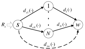
Figure 8: Oligopoly with an overflow link.

Such an oligopoly is essentially the same as those studied in Section III with the exception that $s$ now has the additional option of sending traffic on link $(s,w)$. From a pricing perspective, we can think of $w$ as directly competing with relays by using a uniformly-zero pricing function.

In a general pricing game, the introduction of the overflow link affects only the local competition faced by $i\in{\cal O}_{s}$. Now $w$ becomes a new competitor to all $i\in{\cal O}_{s}$ whose presence changes each $i$’s perception of the competition. Specifically, the pricing function of $i$’s virtual competitor is derived as

$$B_{\hat{i}}^{s}(r)=\min\sum_{j\in{\cal S}_{i}^{s}}B_{j}^{h}(f_{sj})+D_{sw}(f_{sw}),$$

where the minimization is taken with respect to nonnegative $((f_{sj})_{j\in{\cal S}_{i}^{s}},f_{sw})$ such that $\sum_{j}f_{sj}+f_{sw}=r$. The conclusions for pricing games with an elastic source are almost verbatim to those for inelastic pricing games. Limited by space, we do not elaborate further.

VI Conclusion

This work presented a game-theoretic analysis of price competition in multi-hop relay networks. The introduction of possibly nonlinear pricing functions to the game enabled us to develop a much richer set of results than if we allowed only constant unit prices. While the socially optimal routing can always be induced by an equilibrium, the game may have inefficient equilibria as well. Furthermore, the existence of competition turns out to be a two-sided coin. On the one side, any competitive equilibrium in oligopoly pricing games and any everywhere competitive equilibrium in general pricing games must be efficient. On the other side, the conclusion that the price of anarchy of an oligopoly is equal to the number of competitors seems to suggest that more intense competition only makes inefficient (monopolistic) equilibria even worse. Unlike the case of oligopolies, the inefficiency of equilibria in a general pricing game can be attributed not only to manipulative pricing by dominant relays, but also more fundamentally, to the myopia of dominant relays. We showed that the price of anarchy attributed to both the monopolistic and myopic effects is unbounded.

-A Proof of Theorem 8

We prove the theorem by constructing an equilibrium that supports the socially optimal routing. Let $(f_{hi}^{*})$ be the link flows of the socially optimal routing. Denote the total incoming flow at node $i$ by $r_{i}^{*}\triangleq\sum_{h\in{\cal P}_{i}}f_{hi}^{*}$. Note that under the socially optimal routing, a path/sub-path has positive flow only if it has the minimum marginal cost among all paths/sub-paths with the same origin. Let $\lambda_{i}^{*}$ denote the minimum marginal cost of any path/sub-path from $i$ to $w$ (for $i=w$, $\lambda_{i}^{*}=0$). Consider the following pricing scheme. Each relay $i$ adopts $\beta_{i}^{h}(t)\equiv\lambda_{h}^{*}$ for any $h\in{\cal P}_{i}$ unless $r_{h}^{*}=0$, in which case honest pricing $\beta_{i}^{h}(t)=d_{hi}(t)+d_{i}(r_{i}^{*}+t)$ is enforced. Such a pricing scheme will be referred to as marginal cost pricing. We show that marginal cost pricing supports the socially optimal routing. That is, for any relay $i$, given that each $h\in{\cal P}_{i}$ has total traffic $r_{h}^{*}$ to allocate and every relay $j\in{\cal S}_{i}^{h}$ adopts $\beta_{j}^{h}(t)\equiv\lambda_{h}^{*}$ (if $w\in{\cal S}_{i}^{h}$, it always adopts $\beta_{w}^{h}(t)=d_{hw}(t)$), (1) $\beta_{i}^{h}(t)\equiv\lambda_{h}^{*}$ for each $h\in{\cal P}_{i}$ is a best response and (2) the traffic allocation $(f_{hi}^{*})_{h\in{\cal P}_{i}}$ is the most profitable allocation from $i$’s perspective (cf. Lemma 1).

We will need the following lemmas to prove the theorem.

Lemma 3

Under marginal cost pricing, for each relay $i$, its virtual competitor’s pricing function $B_{\hat{i}}^{h}(\cdot)$ and its minimum outgoing cost function $D_{i}(\cdot)$ are convex.

Lemma 3 is a special case of the next general observation.

Lemma 4

For any $K\in\mathbb{N}$, the function

$$g(x)\triangleq\min_{\begin{subarray}{c}\sum_{i=1}^{K}x_{i}=x\\ x_{i}\in{\cal G}_{i},i=1,\cdots,K\end{subarray}}\sum_{i=1}^{K}g_{i}(x_{i})$$

is convex if every $g_{i}(\cdot)$ with domain ${\cal G}_{i}$ is convex.

Proof: Let $y,z$ be two distinct points in the domain of $g(\cdot)$. For any $\lambda\in[0,1]$, let $\bar{\lambda}$ denote $1-\lambda$. We have

$$\lambda g(y)+\bar{\lambda}g(z) = \lambda\min_{\begin{subarray}{c}\sum_{i}y_{i}=y\\ y_{i}\in{\cal G}_{i}\end{subarray}}\sum_{i}g_{i}(y_{i})+\bar{\lambda}\min_{\begin{subarray}{c}\sum_{i}z_{i}=z\\ z_{i}\in{\cal G}_{i}\end{subarray}}\sum_{i}g_{i}(z_{i})$$

$$\stackrel{{\scriptstyle(a)}}{{=}} \lambda\sum_{i}g_{i}(y_{i}^{*})+\bar{\lambda}\sum_{i}g_{i}(z_{i}^{*})$$

$$\stackrel{{\scriptstyle(b)}}{{\geq}} \sum_{i}g_{i}(\lambda y_{i}^{*}+\bar{\lambda}z_{i}^{*})$$

$$\stackrel{{\scriptstyle(c)}}{{\geq}} \min_{\begin{subarray}{c}\sum_{i}x_{i}=\lambda y+\bar{\lambda}z\\ x_{i}\in{\cal G}_{i}\end{subarray}}\sum_{i}g_{i}(x_{i})=g(\lambda y+\bar{\lambda}z).$$

For equality (a), we assume $(y_{i}^{*})=\arg\min_{\sum_{i}y_{i}=y}\sum_{i}g_{i}(y_{i})$ and $(z_{i}^{*})=\arg\min_{\sum_{i}z_{i}=z}\sum_{i}g_{i}(z_{i})$. Inequality (b) follows from the convexity of each $g_{i}(\cdot)$. Because $\sum_{i}\lambda y_{i}^{*}+\bar{\lambda}z_{i}^{*}=\lambda y+\bar{\lambda}z$ and $\lambda y_{i}^{*}+\bar{\lambda}z_{i}^{*}\in{\cal G}_{i}$ for $i=1,\cdots,K$, we have inequality (c). ∎

Proof of Lemma 3: By definition,

$$B_{\hat{i}}^{h}(t)=\min_{\sum_{j\in{\cal S}_{i}^{h}}f_{hj}=t}\sum_{j\in{\cal S}_{i}^{h}}B_{j}^{h}(f_{hj}),$$

where $B_{j}^{h}(t)=\int_{0}^{t}\beta_{j}^{h}(r)~{}dr$. Under marginal cost pricing $\beta_{j}^{h}(r)\equiv\lambda_{h}^{*}$ if $j$ is a relay or $\beta_{j}^{h}(r)=d_{hj}(r)$ if $j$ is the destination, in either case $B_{j}^{h}(t)$ is convex. So $B_{\hat{i}}^{h}(t)$ is convex by Lemma 4. Similarly, we have

$$D_{i}(t)=\min_{\sum_{k\in{\cal O}_{i}}f_{ik}=t}\sum_{k\in{\cal O}_{i}}B_{k}^{i}(f_{ik}),$$

which is convex also because each $B_{k}^{i}(t)$ is convex. ∎

Lemma 3 implies that under marginal cost pricing, $\beta_{\hat{i}}^{h}(t)=\frac{d}{dt}B_{\hat{i}}^{h}(t)$ and $d_{i}(t)=\frac{d}{dt}D_{i}(t)$ are nondecreasing for all relays $i$ and all $h\in{\cal P}_{i}$. In fact, $\beta_{\hat{i}}^{h}(t)$ and $d_{i}(t)$ have the following characterization.

Lemma 5

Under marginal cost pricing, $\beta_{\hat{i}}^{h}(t)$ of any relay $i$ and any $h\in{\cal P}_{i}$ with positive incoming traffic can be expressed as

$$\beta_{\hat{i}}^{h}(t)=\left\{\begin{array}[]{ll}\lambda_{h}^{*},&\textrm{if}~{}w\notin{\cal S}_{i}^{h}\\ \min(d_{hw}(t),\lambda^{*}_{h}),&\textrm{otherwise}\end{array}\right.,$$ (12)

and if $i$ has positive incoming traffic, then $d_{i}(t)$ can be expressed as

$$d_{i}(t)=\left\{\begin{array}[]{ll}\lambda_{i}^{*},&\textrm{if}~{}w\notin{\cal O}_{i}\\ d_{iw}(t),&\textrm{if}~{}{\cal O}_{i}=\{w\}\\ \min(d_{iw}(t),\lambda^{*}_{i}),&\textrm{otherwise}\end{array}\right..$$ (13)

Proof: First, by assumption, ${\cal S}_{i}^{h}$ contains at least one relay and every relay $j$ in ${\cal S}_{i}^{h}$ applies $\beta_{j}^{h}(t)\equiv\lambda_{h}^{*}$. If $w\notin{\cal S}_{i}^{h}$, the (marginal) pricing function of $i$’s virtual competitor is nothing but $\beta_{\hat{i}}^{h}(t)\equiv\lambda_{h}^{*}$. However, if $w\in{\cal S}_{i}^{h}$, it always adopts $\beta_{w}^{h}(t)=d_{hw}(t)$. Thus, the pricing function of $i$’s virtual competitor is

$$B_{\hat{i}}^{h}(t)=\min_{x+y=t}\int_{0}^{x}d_{hw}(r)~{}dr+\int_{0}^{y}\lambda_{h}^{*}~{}dr.$$

Because $d_{hw}(r)$ is increasing, $\beta_{\hat{i}}^{h}(t)=\frac{d}{dt}B_{\hat{i}}^{h}(t)=\min(d_{hw}(t),\lambda_{h}^{*})$. The derivation of (13) is almost verbatim, and we we skip it for brevity. ∎

While Lemma 5 provides general expressions for $\beta_{\hat{i}}^{h}(t)$ and $d_{i}(t)$ under marginal cost pricing, the following lemma specifies the values of the two functions evaluated at the optimal routing configuration, i.e., $\beta_{\hat{i}}^{h}(r_{h}^{*}-f_{hi}^{*})$ and $d_{i}(r_{i}^{*})$. These values are crucial to determining a best response $\beta_{i}^{h}(\cdot)$ for all $h\in{\cal P}_{i}$.

Lemma 6

Under marginal cost pricing and at the socially optimal routing $(f_{mn}^{*})_{(m,n)\in{\cal E}}$ with $r_{n}^{*}=\sum_{m\in{\cal P}_{n}}f_{mn}^{*}$, $n\in{\cal N}$, we have for any relay $i$ and any $h\in{\cal P}_{i}$, $\beta_{\hat{i}}^{h}(r_{h}^{*}-f_{hi}^{*})=\lambda_{h}^{*}$ and $d_{i}(r_{i}^{*})=\lambda_{i}^{*}$. Furthermore, $\beta_{\hat{i}}^{h}(t)\equiv\lambda_{h}^{*}$ for $t\in[r_{h}^{*}-f_{hi}^{*},r_{h}^{*}]$.

Proof: By (12), $\beta_{\hat{i}}^{h}(r_{h}^{*}-f_{hi}^{*})$ can be evaluated as follows:

$$\beta_{\hat{i}}^{h}(r_{h}^{*}-f_{hi}^{*})=\left\{\begin{array}[]{ll}\lambda_{h}^{*},&\textrm{if}~{}w\notin{\cal S}_{i}^{h}\\ \min(d_{hw}(r_{h}^{*}-f_{hi}^{*}),\lambda^{*}_{h})=\lambda^{*}_{h},&\textrm{otherwise}\end{array}\right.,$$

where the second equality holds since $d_{hw}(r_{h}^{*}-f_{hi}^{*})\geq d_{hw}(f_{hw}^{*})\geq\lambda_{h}^{*}$. So in summary, $\beta_{\hat{i}}^{h}(r_{h}^{*}-f_{hi}^{*})=\lambda^{*}_{h}$ under all circumstances. Moreover, (12) also implies that $\beta_{\hat{i}}^{h}(t)\leq\lambda_{h}^{*}$ for all $t\in[0,r_{h}^{*}]$. However, $\beta_{\hat{i}}^{h}(t)$ is nondecreasing as a result of Lemma 3. Thus, $\beta_{\hat{i}}^{h}(t)\equiv\lambda_{h}^{*}$ for $t\in[r_{h}^{*}-f_{hi}^{*},r_{h}^{*}]$.

Next we show that under marginal cost pricing, $d_{i}(r_{i}^{*})=\lambda_{i}^{*}$ for all nodes $i$. Let’s first assume $r_{i}^{*}>0$ and use the expression (13). If ${\cal O}_{i}=\{w\}$, $d_{i}(t)=\beta_{w}^{i}(t)=d_{iw}(t)$. In this case, $f_{iw}^{*}=r_{i}^{*}$ and so $d_{i}(r_{i}^{*})=d_{iw}(f_{iw}^{*})=\lambda_{i}^{*}$. If $w\notin{\cal O}_{i}$, then all the offsprings of $i$ announce $\beta_{j}^{i}(\cdot)\equiv\lambda_{i}^{*}$, thus $d_{i}(\cdot)\equiv\lambda_{i}^{*}$. Finally, if both $w$ and some relay $j$ are in ${\cal O}_{i}$, then $d_{i}(t)=\min(d_{iw}(t),\lambda_{i}^{*})$. Because $d_{iw}(r_{i}^{*})\geq d_{iw}(f_{iw}^{*})\geq\lambda_{i}^{*}$, we have $d_{i}(r_{i}^{*})=\min(d_{iw}(r_{i}^{*}),\lambda_{i}^{*})=\lambda_{i}^{*}$. So we are done with the case $r_{i}^{*}>0$.

If $r_{i}^{*}=0$, every offspring $j$ of $i$ adopts honest pricing $\beta_{j}^{i}(t)=d_{ij}(t)+d_{j}(r_{j}^{*}+t)$ (and $\beta_{w}^{i}(t)=d_{iw}(t)$ if $w\in{\cal O}_{i}$). Thus, by defining $d_{w}(\cdot)\equiv 0$, we can express $d_{i}(r_{i}^{*})$ as

$$d_{i}(r_{i}^{*})=d_{i}(0)=\min_{j\in{\cal O}_{i}}\beta_{j}^{i}(0)=\min_{j\in{\cal O}_{i}}d_{ij}(0)+d_{j}(r_{j}^{*}).$$

If $d_{j}(r_{j}^{*})=\lambda_{j}^{*}$ for all $j\in{\cal O}_{i}$, $d_{i}(r_{i}^{*})$ must be equal to $\lambda_{i}^{*}$. So far we have shown that $d_{j}(r_{j}^{*})=\lambda_{j}^{*}$ if $r_{j}^{*}>0$. Should $r_{j}^{*}=0$ for some $j\in{\cal O}_{i}$, we can evaluate $d_{j}(r_{j}^{*})$ by $d_{j}(r_{j}^{*})=d_{j}(0)=\min_{k\in{\cal O}_{j}}d_{jk}(0)+d_{k}(r_{k}^{*})$. If $r_{k}^{*}>0$ for all $k\in{\cal O}_{j}$, then we will be able to show that $d_{j}(r_{j}^{*})=\lambda_{j}^{*}$. Otherwise, we further expand those $d_{k}(r_{k}^{*})$ such that $r_{k}^{*}=0$. Because the routing topology is loop-free, eventually the recursive evaluation will terminate (either when all offsprings have positive incoming traffic or when the destination is the only offspring). Then calculating in the reverse order of the recursive expansion, we can in the end show that $d_{i}(r_{i}^{*})=\lambda_{i}^{*}$ even if $r_{i}^{*}=0$. So the proof is complete. ∎

Now we are ready to apply Lemma 1 to show that (1) using $\beta_{i}^{h}(t)\equiv\lambda_{h}^{*}$ for all $h\in{\cal P}_{i}$ is a best response of $i$ given each $h\in{\cal P}_{i}$ has total traffic $r_{h}^{*}$ and its competitors all adopt marginal cost pricing and (2) this best response induces traffic allocation $(f_{hi}^{*})_{h\in{\cal P}_{i}}$.

Proof of Theorem 8:

Step 1: Referring to Lemma 1, we first show that $(f_{hi}^{*})_{h\in{\cal P}_{i}}$ maximizes

$$\bar{\Gamma}_{i}(\boldsymbol{f}_{i};\boldsymbol{L}_{i}) = \sum_{h\in{\cal P}_{i}}\left[B_{\hat{i}}^{h}(r_{h}^{*})-B_{\hat{i}}^{h}(r_{h}^{*}-f_{hi})-D_{hi}(f_{hi})\right]-D_{i}\left(\sum_{h\in{\cal P}_{i}}f_{hi}\right)$$

$$= \sum_{h\in{\cal P}_{i}}\int_{0}^{f_{hi}}\beta_{\hat{i}}^{h}(r_{h}^{*}-t)-d_{hi}(t)~{}dt-\int_{0}^{\sum_{h\in{\cal P}_{i}}f_{hi}}d_{i}(t)~{}dt$$

over all the $\boldsymbol{f}_{i}=(f_{hi})$ such that $0\leq f_{hi}\leq r_{h}^{*}$ for all $h\in{\cal P}_{i}$.

Note that if $f_{hi}^{*}>0$, $i$ must be on a sub-path from $h$ to $w$ with the minimum marginal cost, so $\lambda_{h}^{*}=d_{hi}(f_{hi}^{*})+\lambda_{i}^{*}$. Otherwise, $\lambda_{h}^{*}\leq d_{hi}(f_{hi}^{*})+\lambda_{i}^{*}$. Therefore, we can conclude that

$$(f_{hi}^{*})_{h\in{\cal P}_{i}} = \mathop{\arg\max}_{\begin{subarray}{c}0\leq f_{hi}\leq r_{h}^{*}\\ h\in{\cal P}_{i}\end{subarray}}\left\{\sum_{h\in{\cal P}_{i}}\int_{0}^{f_{hi}}\beta_{\hat{i}}^{h}(r_{h}^{*}-t)-d_{hi}(t)-d_{i}(r_{i}^{*}-f_{hi}^{*}+t)~{}dt\right\}$$

$$= \mathop{\arg\max}_{\begin{subarray}{c}0\leq f_{hi}\leq r_{h}^{*}\\ h\in{\cal P}_{i}\end{subarray}}\left\{\bar{\Gamma}_{i}(\boldsymbol{f}_{i};\boldsymbol{L}_{i})+\int_{0}^{\sum_{h\in{\cal P}_{i}}f_{hi}}d_{i}(t)~{}dt-\sum_{h\in{\cal P}_{i}}\int_{0}^{f_{hi}}d_{i}(r_{i}^{*}-f_{hi}^{*}+t)~{}dt\right\}$$

$$\triangleq \mathop{\arg\max}_{\begin{subarray}{c}0\leq f_{hi}\leq r_{h}^{*}\\ h\in{\cal P}_{i}\end{subarray}}\left\{\bar{\Gamma}_{i}(\boldsymbol{f}_{i};\boldsymbol{L}_{i})+\Delta(\boldsymbol{f}_{i})\right\}.$$

The first equality follows from the fact that $\beta_{\hat{i}}^{h}(r_{h}^{*}-t)-d_{hi}(t)-d_{i}(r_{i}^{*}-f_{hi}^{*}+t)$ is nonincreasing in $t$ (by Lemma 3) and that

$$\beta_{\hat{i}}^{h}(r_{h}^{*}-f_{hi}^{*})-d_{hi}(f_{hi}^{*})-d_{i}(r_{i}^{*})\left\{\begin{array}[]{ll}\leq 0,&f_{hi}^{*}=0\\ =0,&0<f_{hi}^{*}\leq r_{m}^{*}\end{array}\right.,$$ (14)

which follows from Lemma 6. The second and third equalities are by regrouping terms and defining the terms other than $\bar{\Gamma}_{i}(\boldsymbol{f}_{i};\boldsymbol{L}_{i})$ to be $\Delta(\boldsymbol{f}_{i})$. We can rewrite $\Delta(\boldsymbol{f}_{i})$ as

$$\Delta(\boldsymbol{f}_{i})=\int_{0}^{r_{i}}d_{i}(t)~{}dt-\sum_{h\in{\cal P}_{i}}\int_{r_{i}^{*}-f_{hi}^{*}}^{r_{i}^{*}-f_{hi}^{*}+f_{hi}}d_{i}(t)~{}dt.$$

Now consider the difference

$$\Delta(\boldsymbol{f}_{i})-\Delta(\boldsymbol{f}_{i}^{*})=\int_{r_{i}^{*}}^{r_{i}}d_{i}(t)~{}dt-\sum_{h\in{\cal P}_{i}}\int_{r_{i}^{*}}^{r_{i}^{*}-f_{hi}^{*}+f_{hi}}d_{i}(t)~{}dt.$$

Recall that $d_{i}(\cdot)$ is positive and nondecreasing. If $f_{hi}\geq f_{hi}^{*}$ for all $h\in{\cal P}_{i}$, then the difference is easily seen to be nonnegative. If $f_{hi}\leq f_{hi}^{*}$ for all $h\in{\cal P}_{i}$, we can rewrite the difference as

$$\Delta(\boldsymbol{f}_{i})-\Delta(\boldsymbol{f}_{i}^{*})=\sum_{h\in{\cal P}_{i}}\int_{r_{i}^{*}-f_{hi}^{*}+f_{hi}}^{r_{i}^{*}}d_{i}(t)~{}dt-\int_{r_{i}}^{r_{i}^{*}}d_{i}(t)~{}dt,$$

which, by the same reason, is nonnegative.

To summarize, the function $\Delta(\boldsymbol{f}_{i})$ is minimized at $\boldsymbol{f}_{i}^{*}$ within the region ${\cal F}(\boldsymbol{f}_{i}^{*})\triangleq\{\boldsymbol{f}_{i}:f_{hi}\geq f_{hi}^{*},\forall h\in{\cal P}_{i}~{}\textrm{or}~{}f_{hi}\leq f_{hi}^{*},\forall h\in{\cal P}_{i}\}$. Thus, it can be concluded that $\bar{\Gamma}_{i}(\boldsymbol{f}_{i};\boldsymbol{L}_{i})$ must be maximized at $\boldsymbol{f}_{i}^{*}$ within ${\cal F}(\boldsymbol{f}_{i}^{*})$. Recall that the feasible region for the maximization of $\bar{\Gamma}_{i}(\boldsymbol{f}_{i};\boldsymbol{L}_{i})$ is ${\cal F}_{i}=\{\boldsymbol{f}_{i}:0\leq f_{hi}\leq r_{h}^{*},\forall h\in{\cal P}_{i}\}$. Next we show that the maximizer of $\bar{\Gamma}_{i}(\boldsymbol{f}_{i};\boldsymbol{L}_{i})$ cannot lie in ${\cal F}^{c}(\boldsymbol{f}_{i}^{*})\triangleq{\cal F}_{i}\backslash{\cal F}(\boldsymbol{f}_{i}^{*})$.

Suppose $\bar{\Gamma}_{i}(\boldsymbol{f}_{i};\boldsymbol{L}_{i})$ is maximized at $\bar{\boldsymbol{f}_{i}}$. Then at the maximum it must hold for all $h\in{\cal P}_{i}$ that

$$\frac{\partial}{\partial f_{hi}}\bar{\Gamma}_{i}(\bar{\boldsymbol{f}_{i}};\boldsymbol{L}_{i})=\beta_{\hat{i}}^{h}(r_{h}^{*}-\bar{f}_{hi})-d_{hi}(\bar{f}_{hi})-d_{i}(\bar{r}_{i})\left\{\begin{array}[]{ll}\leq 0,&\bar{f}_{hi}=0\\ =0,&0<\bar{f}_{hi}<r_{h}^{*}\\ \geq 0,&\bar{f}_{hi}=r_{h}^{*}\end{array}\right.,$$

or equivalently

$$\beta_{\hat{i}}^{h}(r_{h}^{*}-\bar{f}_{hi})-d_{hi}(\bar{f}_{hi})\left\{\begin{array}[]{ll}\leq d_{i}(\bar{r}_{i}),&\bar{f}_{hi}=0\\ =d_{i}(\bar{r}_{i}),&0<\bar{f}_{hi}<r_{h}^{*}\\ \geq d_{i}(\bar{r}_{i}),&\bar{f}_{hi}=r_{h}^{*}\end{array}\right.,$$ (15)

where $\bar{r}_{i}=\sum_{h}\bar{f}_{hi}$. It is straightforward to verify that $\boldsymbol{f}_{i}^{*}$ is a solution to the above simultaneous formulas (cf (14)). Next we demonstrate that there is no other solution in ${\cal F}^{c}(\boldsymbol{f}_{i}^{*})$. First, if $f_{hi}^{*}=0$ for all $h\in{\cal P}_{i}$ or if $f_{hi}^{*}=r_{h}^{*}$ for all $h\in{\cal P}_{i}$, then ${\cal F}^{c}(\boldsymbol{f}_{i}^{*})$ is empty, so we are done. Otherwise, let ${\cal P}_{i}^{0}\triangleq\{h\in{\cal P}_{i}:f_{hi}^{*}=0\}$, ${\cal P}_{i}^{+}\triangleq\{h\in{\cal P}_{i}:f_{hi}^{*}=r_{h}^{*}\}$. Hence, for those $h\in{\cal P}_{i}\backslash({\cal P}_{i}^{0}\cup{\cal P}_{i}^{+})$, $f_{hi}^{*}$ is in the interior of $[0,r_{h}^{*}]$. Accordingly, the simultaneous formulas satisfied by $\boldsymbol{f}_{i}^{*}$ are

$$\beta_{\hat{i}}^{h}(r_{h}^{*})-d_{hi}(0) \leq d_{i}(r_{i}^{*}),\quad h\in{\cal P}_{i}^{0},$$

$$\beta_{\hat{i}}^{h}(r_{h}^{*}-f_{hi}^{*})-d_{hi}(f_{hi}^{*}) \geq d_{i}(r_{i}^{*}),\quad h\in{\cal P}_{i}^{+},$$

$$\beta_{\hat{i}}^{h}(0)-d_{hi}(r_{h}^{*}) = d_{i}(r_{i}^{*}),\quad\textrm{otherwise}.$$

Now suppose there is a different solution $\boldsymbol{f}_{i}^{\prime}$ in ${\cal F}^{c}(\boldsymbol{f}_{i}^{*})$ such that for some $a,b\in{\cal P}_{i}$, $f_{ai}^{\prime}>f_{ai}^{*}$ and $f_{bi}^{\prime}<f_{bi}^{*}$. It follows that $a\notin{\cal P}_{i}^{+}$ and $b\notin{\cal P}_{i}^{0}$. Hence, $\beta_{\hat{i}}^{a}(r_{a}^{*}-f_{ai}^{*})-d_{ai}(f_{ai}^{*})\leq\beta_{\hat{i}}^{b}(r_{b}^{*}-f_{bi}^{*})-d_{bi}(f_{bi}^{*})$. Because $\beta_{\hat{i}}^{h}(r_{h}^{*}-f_{hi})-d_{hi}(f_{hi})$ is strictly decreasing with $f_{hi}$ for all $h\in{\cal P}_{i}$, we must have $\beta_{\hat{i}}^{a}(r_{a}^{*}-f_{ai}^{\prime})-d_{ai}(f_{ai}^{\prime})<\beta_{\hat{i}}^{b}(r_{b}^{*}-f_{bi}^{\prime})-d_{bi}(f_{bi}^{\prime})$. However, since $f_{ai}^{\prime}>0$, $f_{bi}^{\prime}<r_{b}^{*}$, and they satisfy the respective formulas in (15), it follows that

$$\beta_{\hat{i}}^{a}(r_{a}^{*}-f_{ai}^{\prime})-d_{ai}(f_{ai}^{\prime})\geq d_{i}(r_{i}^{\prime})\geq\beta_{\hat{i}}^{b}(r_{b}^{*}-f_{bi}^{\prime})-d_{bi}(f_{bi}^{\prime}),$$

thus, a contradiction. Therefore, we have shown that no solution exists in ${\cal F}^{c}(\boldsymbol{f}_{i}^{*})$.

To recap, the maximizer of $\bar{\Gamma}_{i}(\boldsymbol{f}_{i};\boldsymbol{L}_{i})$ must fall in ${\cal F}(\boldsymbol{f}_{i}^{*})$. Moreover, we have found that $\boldsymbol{f}_{i}^{*}$ maximizes $\bar{\Gamma}_{i}(\boldsymbol{f}_{i};\boldsymbol{L}_{i})$ within ${\cal F}(\boldsymbol{f}_{i}^{*})$. So we can conclude that

$$\boldsymbol{f}_{i}^{*}=\mathop{\arg\max}_{{\cal F}_{i}}\bar{\Gamma}_{i}(\boldsymbol{f}_{i};\boldsymbol{L}_{i}).$$

Step 2: Next we show that condition (4) holds with $\beta_{i}^{h}(t)\equiv\lambda_{h}^{*}$, i.e,

$$B_{i}^{h}(t)\geq B_{\hat{i}}^{h}(r_{h}^{*})-B_{\hat{i}}^{h}(r_{h}^{*}-t)$$

for all $h\in{\cal P}_{i}$ and all $t\in[0,r_{h}^{*}]$. Since $\beta_{i}^{h}(t)\equiv\lambda_{h}^{*}$, LHS is $B_{i}^{h}(t)=\int_{0}^{t}\beta_{i}^{h}(r)~{}dr=\lambda_{h}^{*}t$. By the expression (12), $\beta_{\hat{i}}^{h}(t)\leq\lambda_{h}^{*}$ under all circumstances. So the RHS of the above inequality is $B_{\hat{i}}^{h}(r_{h}^{*})-B_{\hat{i}}^{h}(r_{h}^{*}-t)=\int_{r_{h}^{*}-t}^{r_{h}^{*}}\beta_{\hat{i}}^{h}(r)~{}dr\leq\lambda_{h}^{*}t$. And this proves (4).

Step 3: Finally, we prove that condition (5) is established by the combination of the pricing function $\beta_{i}^{h}(t)\equiv\lambda_{h}^{*}$ and the traffic allocation $f_{hi}^{*}$, i.e., for all $h\in{\cal P}_{i}$,

$$B_{i}^{h}(f_{hi}^{*})=B_{\hat{i}}^{h}(r_{h}^{*})-B_{\hat{i}}^{h}(r_{h}^{*}-f_{hi}^{*}).$$

Note that the LHS is equal to $B_{i}^{h}(f_{hi}^{*})=\int_{0}^{f_{hi}^{*}}\beta_{i}^{h}(r)~{}dr=\lambda_{h}^{*}f_{hi}^{*}$. By Lemma 6, $\beta_{\hat{i}}^{h}(t)\equiv\lambda_{h}^{*}$ for $t\in[r_{h}^{*}-f_{hi}^{*},r_{h}^{*}]$. It follows that $B_{\hat{i}}^{h}(r_{h}^{*})-B_{\hat{i}}^{h}(r_{h}^{*}-f_{hi}^{*})=\int_{r_{h}^{*}-f_{hi}^{*}}^{r_{h}^{*}}\beta_{\hat{i}}^{h}(r)~{}dr=\lambda_{h}^{*}f_{hi}^{*}$. So (5) is proved.

Conclusion: With all the necessary and sufficient conditions in Lemma 1 satisfied, we can conclude that $\beta_{i}^{h}(t)\equiv\lambda_{h}^{*}$ for all $h\in{\cal P}_{i}$ is a best response of $i$ given that all its competitors also adopt marginal cost pricing. Furthermore, the socially optimal routing $(f_{hi}^{*})$ is the traffic allocation induced by the equilibrium under marginal cost pricing. Therefore, the proof for Theorem 8 is complete. ∎

-B Proof of Theorem 9

We use the following lemmas to prove the theorem.

Lemma 7

Given any (focal) equilibrium with induced link flows $(f_{hi})$ and node total incoming rates $(r_{i})$, for any node $i$ with $r_{i}\in(0,R_{s})$, its actual marginal cost $\lambda_{i}^{h}(\cdot)$ of forwarding traffic for any $h\in{\cal P}_{i}$ (with $f_{h^{\prime}i}$ of all other $h^{\prime}\in{\cal P}_{i}$ fixed) satisfies

$$\lambda_{i}^{h}(f_{hi})^{+}\leq\lambda_{i}^{h}(f_{hi})^{-},$$ (16)

where $\lambda_{i}^{h}(f_{hi})^{+}$ and $\lambda_{i}^{h}(f_{hi})^{-}$ are the right and left limits of $\lambda_{i}^{h}(\cdot)$ at $f_{hi}$.

Proof: First assume that $i$ has only one offspring, which by our assumption must be the destination. Thus, $\lambda_{i}^{h}(t)=d_{hi}(t)+d_{iw}(t)$. Since both $d_{hi}(\cdot)$ and $d_{iw}(\cdot)$ are continuous everywhere, $\lambda_{i}^{h}(\cdot)$ must also be continuous everywhere. The inequality (16) holds with equality.

Next assume that $i$ has multiple offsprings. By the same reasoning as used in the proof of Lemma 2, for any $j\in{\cal O}_{i}$ with $f_{ij}>0$, we have

$$\lambda_{i}^{h}(f_{hi})^{+}\leq d_{hi}(f_{hi})+\beta_{\hat{j}}^{i}(r_{i}-f_{ij})^{+}=d_{hi}(f_{hi})+\beta_{j}^{i}(f_{ij})^{-}\leq\lambda_{i}^{h}(f_{hi})^{-},$$

where the equality follows from the replicating response $\beta_{j}^{i}(t)=\beta_{\hat{j}}^{i}(r_{i}-t),~{}t\in[0,f_{ij}]$, assumed by a focal equilibrium. ∎

Lemma 8

Given any (focal) equilibrium with induced link flows $(f_{hi})$ and node total incoming rates $(r_{i})$, for any $h\neq w$ such that $f_{hi}>0$ and $f_{hj}>0$ for two different relays $i,j\in{\cal O}_{h}$, it holds that

(i) the actual marginal cost $\lambda_{i}^{h}(\cdot)$, $\lambda_{j}^{h}(\cdot)$ of $i$ and $j$ forwarding traffic for $h$ are continuous at $f_{hi}$ and $f_{hj}$, respectively;

(ii) the marginal pricing functions $\beta_{\hat{i}}^{h}(\cdot)$, $\beta_{\hat{j}}^{h}(\cdot)$ of $i$ and $j$’s virtual competitors are continuous at $r_{h}-f_{hi}$ and $r_{h}-f_{hj}$, respectively;

(iii)

$$\lambda_{i}^{h}(f_{hi})=\lambda_{j}^{h}(f_{hj})=\beta_{\hat{i}}^{h}(r_{h}-f_{hi})=\beta_{\hat{j}}^{h}(r_{h}-f_{hj})\triangleq\eta_{h}.$$

Proof: The replicating response implies $\beta_{i}^{h}(f_{hi})^{-}=\beta_{\hat{i}}^{h}(r_{h}-f_{hi})^{+}$. The fact that

$$f_{hi}=\mathop{\arg\max}_{0\leq f\leq r_{h}}\int_{0}^{f}\beta_{\hat{i}}^{h}(r_{h}-r)-\lambda_{i}^{h}(r)~{}dr$$

implies $\beta_{\hat{i}}^{h}(r_{h}-f_{hi})^{+}\geq\lambda_{i}(f_{hi})^{-}$ and $\lambda_{i}(f_{hi})^{+}\geq\beta_{\hat{i}}^{h}(r_{h}-f_{hi})^{-}$. By the same reasoning as used in the proof of Lemma 2, it can be shown that $\beta_{\hat{i}}^{h}(r_{h}-f_{hi})^{-}\geq\beta_{j}^{h}(f_{hj})^{-}$. Invoking Lemma 7, we have

$$\beta_{i}^{h}(f_{hi})^{-}=\beta_{\hat{i}}^{h}(r_{h}-f_{hi})^{+}\geq\lambda_{i}^{h}(f_{hi})^{-}\geq\lambda_{i}^{h}(f_{hi})^{+}\geq\beta_{\hat{i}}^{h}(r_{h}-f_{hi})^{-}\geq\beta_{j}^{h}(f_{hj})^{-}.$$ (17)

By symmetry,

$$\beta_{j}^{h}(f_{hj})^{-}=\beta_{\hat{j}}^{h}(r_{h}-f_{hj})^{+}\geq\lambda_{j}^{h}(f_{hj})^{-}\geq\lambda_{j}^{h}(f_{hj})^{+}\geq\beta_{\hat{j}}^{h}(r_{h}-f_{hj})^{-}\geq\beta_{i}^{h}(f_{hi})^{-}.$$

Thus, it can be concluded that all terms involved in the above two inequalities must be equal to each other. So the proof is complete. ∎

Lemma 9

Given any (focal) equilibrium with induced link flows $(f_{hi})$ and node total incoming rates $(r_{i})$, for any $h\neq w$ such that $f_{hw}>0$ and $f_{hi}>0$ for a relay $i\in{\cal O}_{h}$, it holds that

(i) the actual marginal cost $\lambda_{w}^{h}(\cdot)$, $\lambda_{i}^{h}(\cdot)$ of $w$ and $i$ forwarding traffic for $h$ are continuous at $f_{hw}$ and $f_{hi}$, respectively;

(ii) the marginal pricing functions $\beta_{\hat{i}}^{h}(\cdot)$ of $i$’s virtual competitor is continuous at $r_{h}-f_{hi}$;

(iii)

$$\lambda_{i}^{h}(f_{hi})=\beta_{\hat{i}}^{h}(r_{h}-f_{hi}).$$

Proof: First of all, $w$ always uses honest pricing, i.e., $\beta_{w}^{h}(\cdot)=\lambda_{w}^{h}(\cdot)=d_{hw}(\cdot)$. So $\lambda_{w}^{h}(\cdot)$ and $\beta_{w}^{h}(\cdot)$ are continuous everywhere. For the relay $i$, the inequality (17) holds with $j$ being replaced by $w$. Also notice that $\beta_{i}^{h}(f_{hi})^{-}\leq\beta_{w}^{h}(f_{hw})^{+}$. For otherwise, $h$ would be able to strictly reduce its total cost by shifting an infinitesimal amount of flow from $(h,i)$ to $(h,w)$. However, since $\beta_{w}^{h}(\cdot)$ is continuous, $\beta_{w}^{h}(f_{hw})^{+}=\beta_{w}^{h}(f_{hw})^{-}$. It follows that all the inequalities in (17) must hold with equality. So the proof is complete. ∎

Lemma 10

At an everywhere competitive equilibrium, all the paths with positive flow have equal marginal cost.

Proof: Let $s,n_{1},n_{2},\cdots,n_{k},w$ be the nodes on a path ${\cal R}$ with positive flow at the equilibrium. For simplicity, denote $s$ by $n_{0}$ and $w$ by $n_{k+1}$. So $f_{n_{i}n_{i+1}}>0$ for all $i=0,1,\cdots,k$.

At the equilibrium we must have for all $i=1,\cdots,k-1$,

$$\lambda_{n_{i}}^{n_{i-1}}(f_{n_{i-1}n_{i}})^{-}\stackrel{{\scriptstyle(a)}}{{\geq}}d_{n_{i-1}n_{i}}(f_{n_{i-1}n_{i}})+\beta_{n_{i+1}}^{n_{i}}(f_{n_{i}n_{i+1}})^{-} \stackrel{{\scriptstyle(b)}}{{=}} d_{n_{i-1}n_{i}}(f_{n_{i-1}n_{i}})+\beta_{\hat{n}_{i+1}}^{n_{i}}(r_{n_{i}}-f_{n_{i}n_{i+1}})^{+}$$

$$\stackrel{{\scriptstyle(c)}}{{\geq}} d_{n_{i-1}n_{i}}(f_{n_{i-1}n_{i}})+\lambda_{n_{i+1}}^{n_{i}}(f_{n_{i}n_{i+1}})^{-}.$$

We have seen inequality $(a)$ in the proof of Lemma 7. The equality $(b)$ follows from the replicating response. The inequality $(c)$ is due to the fact that $f_{n_{i}n_{i+1}}$ is the ideal flow rate to $n_{i+1}$ given $\beta_{\hat{n}_{i+1}}^{n_{i}}(\cdot)$. Using the above relation successively from $i=1$ to $i=k-1$, we obtain

$$\lambda_{n_{1}}^{s}(f_{sn_{1}})^{-}\geq d_{sn_{1}}(f_{sn_{1}})+d_{n_{1}n_{2}}(f_{n_{1}n_{2}})+\cdots+d_{n_{k-2}n_{k-1}}(n_{k-2}n_{k-1})+\lambda_{n_{k}}^{n_{k-1}}(f_{n_{k-1}n_{k}})^{-}.$$

Finally notice that $\beta_{w}^{n_{k}}(\cdot)=d_{n_{k}w}(\cdot)$, so

$$\lambda_{n_{k}}^{n_{k-1}}(f_{n_{k-1}n_{k}})^{-}\geq d_{n_{k-1}n_{k}}+\beta_{w}^{n_{k}}(f_{n_{k}w})^{-}=d_{n_{k-1}n_{k}}+d_{n_{k}w}(f_{n_{k}w}).$$

Therefore, the marginal cost of path ${\cal R}$ is upper bounded as

$$d_{sn_{1}}(f_{sn_{1}})+d_{n_{1}n_{2}}(f_{n_{1}n_{2}})+\cdots+d_{n_{k-1}n_{k}}(f_{n_{k-1}n_{k}})+d_{n_{k}w}(f_{n_{k}w})\leq\lambda_{n_{1}}^{s}(f_{sn_{1}})^{-}.$$

Furthermore, since the equilibrium is everywhere competitive, there exists a node $n_{i}^{\prime}\neq n_{i}$ for every $i=1,\cdots,k$ such that $f_{n_{i-1}n_{i}^{\prime}}>0$. Using the results of Lemma 8 and 9, we can show that

$$d_{n_{i-1}n_{i}}(f_{n_{i-1}n_{i}})+\lambda_{n_{i+1}}^{n_{i}}(f_{n_{i}n_{i+1}})=d_{n_{i-1}n_{i}}(f_{n_{i-1}n_{i}})+\beta_{\hat{n}_{i+1}}^{n_{i}}(r_{n_{i}}-f_{n_{i}n_{i+1}})\geq\lambda_{n_{i}}^{n_{i-1}}(f_{n_{i-1}n_{i}}),$$

for $i=1,\cdots,k-1$. Applying the above inequality successively from $i=k-1$ to $i=1$, we have

$$d_{sn_{1}}(f_{sn_{1}})+d_{n_{1}n_{2}}(f_{n_{1}n_{2}})+\cdots+d_{n_{k-1}n_{k}}(f_{n_{k-1}n_{k}})+d_{n_{k}w}(f_{n_{k}w})$$

$$= d_{sn_{1}}(f_{sn_{1}})+d_{n_{1}n_{2}}(f_{n_{1}n_{2}})+\cdots+d_{n_{k-1}n_{k}}(f_{n_{k-1}n_{k}})+\beta_{w}^{n_{k}}(f_{n_{k}w})$$

$$\geq d_{sn_{1}}(f_{sn_{1}})+d_{n_{1}n_{2}}(f_{n_{1}n_{2}})+\cdots+\lambda_{n_{k}}^{n_{k-1}}$$

$$\vdots$$

$$\geq \lambda_{n_{1}}^{s}(f_{sn_{1}}).$$

Also by Lemma 8, $\lambda_{n_{1}}^{s}(\cdot)$ is continuous at $f_{sn_{1}}$. Thus, the lower and upper bounds of the total marginal cost of ${\cal R}$ are both equal to $\lambda_{n_{1}}^{s}(f_{sn_{1}})=\eta_{s}$. Since ${\cal R}$ is chosen arbitrarily, we can conclude that all the paths with positive flow have the same marginal cost $\eta_{s}$. ∎

Proof of Theorem 9: By Lemma 10, at an everywhere competitive equilibrium, every path with positive flow has the same marginal cost $\eta_{s}$. To prove that the routing is socially optimal, it remains to show that any path with zero flow has marginal cost greater than or equal to $\eta_{s}$. Let $s,z_{1},\cdots,z_{m},w$ be the nodes on a zero-flow path ${\cal Z}$. To simplify notation, write $s$ as $z_{0}$ and $w$ as $z_{m+1}$. Recall that the flow rate of a path is the minimum of the flow rates on all its links. So there exist link(s) $(z_{i},z_{i+1})$ on ${\cal Z}$ such that $f_{z_{i}z_{i+1}}=0$. Next we show that on path ${\cal Z}$,

$$d_{z_{i-1}z_{i}}(f_{z_{i-1}z_{i}})+\lambda_{z_{i+1}}^{z_{i}}(f_{z_{i}z_{i+1}})^{+}\geq\lambda_{z_{i}}^{z_{i-1}}(f_{z_{i-1}z_{i}})^{+},$$ (18)

where $i=1,\cdots,m$.

Notice that for $i=m$,

$$d_{z_{m-1}z_{m}}(f_{z_{m-1}z_{m}})+\lambda_{z_{m+1}}^{z_{m}}(f_{z_{m}z_{m+1}})^{+}=d_{z_{m-1}z_{m}}(f_{z_{m-1}z_{m}})+d_{z_{m}w}(f_{z_{m}w})\geq\lambda_{z_{m}}^{z_{m-1}}(f_{z_{m-1}z_{m}})^{+}.$$

Now consider any $i=1,\cdots,m-1$. At an everywhere competitive equilibrium, if $f_{z_{i}z_{i+1}}>0$, then there must exist $z_{i+1}^{\prime}\neq z_{i+1}$ for which $f_{z_{i}z_{i+1}^{\prime}}>0$. Applying Lemma 8 or 9, we have

$$d_{z_{i-1}z_{i}}(f_{z_{i-1}z_{i}})+\lambda_{z_{i+1}}^{z_{i}}(f_{z_{i}z_{i+1}})=d_{z_{i-1}z_{i}}(f_{z_{i-1}z_{i}})+\beta_{\hat{z}_{i+1}}^{z_{i}}(r_{z_{i}}-f_{z_{i}z_{i+1}})\geq\lambda_{z_{i}}^{z_{i-1}}(f_{z_{i-1}z_{i}})^{+}.$$

This is a special case of (18) as $\lambda_{z_{i+1}}^{z_{i}}(\cdot)$ is continuous at $f_{z_{i}z_{i+1}}$. If $f_{z_{i}z_{i+1}}=0$, however, we have to consider the following two cases. In the first case, $r_{z_{i}}>0$, so $z_{i}$ has at least two offsprings $z_{i+1}^{\prime}$, $z_{i+1}^{\prime\prime}$ such that $f_{z_{i}z_{i+1}^{\prime}}>0$ and $f_{z_{i}z_{i+1}^{\prime\prime}}>0$. Assume $z_{i+1}^{\prime}\neq w$, we therefore have

$$d_{z_{i-1}z_{i}}(f_{z_{i-1}z_{i}})+\lambda_{z_{i+1}}^{z_{i}}(f_{z_{i}z_{i+1}})^{+} = d_{z_{i-1}z_{i}}(0)+\lambda_{z_{i+1}}^{z_{i}}(0)^{+}$$

$$\stackrel{{\scriptstyle(a)}}{{\geq}} d_{z_{i-1}z_{i}}(0)+\beta_{\hat{z}_{i+1}}^{z_{i}}(r_{z_{i}})^{-}$$

$$\stackrel{{\scriptstyle(b)}}{{\geq}} d_{z_{i-1}z_{i}}(0)+\beta_{z_{i+1}^{\prime}}^{z_{i}}(f_{z_{i}z_{i+1}^{\prime}})^{-}$$

$$\stackrel{{\scriptstyle(c)}}{{=}} d_{z_{i-1}z_{i}}(0)+\beta_{\hat{z}_{i+1}^{\prime}}^{z_{i}}(r_{z_{i}}-f_{z_{i}z_{i+1}^{\prime}})\geq\lambda_{z_{i}}^{z_{i-1}}(f_{z_{i-1}z_{i}})^{+}.$$

Here, inequality $(a)$ holds because $f_{z_{i}z_{i+1}}=0$ is the ideal amount of flow to $z_{i+1}$. We applied the same reasoning as used in the proof of Lemma 2 to get $(b)$. Inequality $(c)$ follows from the replicating response of $z_{i+1}^{\prime}$ and from using Lemma 8 or 9 (depending on whether $z_{i+1}^{\prime}=w$ or not). Next we consider the case where $r_{z_{i}}=0$ and consequently all offsprings of $z_{i}$ adopt honest pricing to $z_{i}$. It follows that

$$d_{z_{i-1}z_{i}}(f_{z_{i-1}z_{i}})+\lambda_{z_{i+1}}^{z_{i}}(f_{z_{i}z_{i+1}})^{+}=d_{z_{i-1}z_{i}}(f_{z_{i-1}z_{i}})+\beta_{z_{i+1}}^{z_{i}}(f_{z_{i}z_{i+1}})^{+}\geq\lambda_{z_{i}}^{z_{i-1}}(f_{z_{i-1}z_{i}})^{+}.$$

So far we have proved (18). Using (18) we can lower bound the marginal cost of ${\cal Z}$ as

$$d_{z_{0}z_{1}}(f_{z_{0}z_{1}})+\cdots+d_{z_{m-1}z_{m}}(f_{z_{m-1}z_{m}})+d_{z_{m}w}(f_{z_{m}w})$$

$$= d_{z_{0}z_{1}}(f_{z_{0}z_{1}})+\cdots+d_{z_{m-1}z_{m}}(f_{z_{m-1}z_{m}})+\lambda_{w}^{z_{m}}(f_{z_{m}w})$$

$$\vdots$$

$$\geq \lambda_{z_{1}}^{s}(f_{sz_{1}})^{+}.$$

If $f_{sz_{1}}>0$, by Lemma 8, $\lambda_{z_{1}}^{s}(\cdot)$ is continuous at $f_{sz_{1}}$ and is equal to $\eta_{s}$. So we are done. If $f_{sz_{1}}=0$, $s$ must have two other offsprings $z_{1}^{\prime}$, $z_{1}^{\prime\prime}$ for which $f_{sz_{1}^{\prime}}>0$, $f_{sz_{1}^{\prime\prime}}>0$. Then we can apply the same argument as we used in inequalities $(a)$-$(c)$ to show that

$$\lambda_{z_{1}}^{s}(f_{sz_{1}})^{+}\geq\beta_{\hat{z}_{1}^{\prime}}^{s}(R_{s}-f_{sz_{1}^{\prime}})=\lambda_{z_{1}^{\prime}}^{s}(f_{sz_{1}^{\prime}}),$$

where $\lambda_{z_{1}^{\prime}}^{s}(f_{sz_{1}^{\prime}})=\eta_{s}$. So we are done.

To summarize, we have shown that at an everywhere competitive equilibrium, every path with positive flow has the same marginal cost $\eta_{s}$; moreover, every path with zero flow has marginal cost greater than or equal to $\eta_{s}$. Therefore, the routing pattern of such an equilibrium is socially optimal. ∎

References

• [1] O. Ileri, S. Mau, and N. Mandayam, “Pricing for enabling forwarding in self-configuring ad hoc networks,” IEEE Journal on Selected Areas in Communications, vol. 23, no. 1, pp. 151–162, 2005.
• [2] A. Blanc, Y. Liu, and A. Vahdat, “Designing incentives for peer-to-peer routing,” in Proceedings of IEEE INFOCOM 2005, vol. 1, Mar. 2005.
• [3] J. Crowcroft, R. Gibbens, F. Kelly, and S. Östring, “Modelling incentives for collaboration in mobile ad hoc networks,” Performance Evaluation, vol. 57, no. 4, pp. 427–439, 2004.
• [4] P. Marbach and Y. Qiu, “Cooperation in wireless ad hoc networks: a market-based approach,” IEEE/ACM Transactions on Networking, vol. 13, pp. 1325–1338, Dec. 2005.
• [5] L. Buttyan and J.-P. Hubaux, Security and Cooperation in Wireless Networks. Cambridge University Press, 2007.
• [6] F. Kelly, A. Maulloo, and D. Tan, “Rate control in communication networks: shadow prices, proportional fairness and stability,” Journal of the Operational Research Society, vol. 49, 1998.
• [7] R. Cole, Y. Dodis, and T. Roughgarden, “Pricing network edges for heterogeneous selfish users.,” in Proceedings of the 35th Annual ACM Symposium on Theory of Computing, pp. 521–530, Jun. 2003.
• [8] T. Roughgarden and E. Tardos, “How bad is selfish routing,” Journal of the ACM, vol. 49, no. 2, pp. 236–259, 2002.
• [9] T. Roughgarden, “Selfish routing with atomic players,” in Proceedings of the sixteenth annual ACM-SIAM symposium on Discrete algorithms, pp. 1184–1185, 2005.
• [10] J. Shu and P. Varaiya, “Pricing network services,” in Proceedings of IEEE INFOCOM 2003, vol. 2, Mar. 2003.
• [11] L. He and J. Walrand, “Pricing differentiated internet services,” in Proceedings of IEEE INFOCOM 2005, vol. 1, Mar. 2005.
• [12] T. Basar and R. Srikant, “Revenue-maximizing pricing and capacity expansion in a many-users regime,” in Proceedings of IEEE INFOCOM 2002, vol. 1, 2002.
• [13] L. He and J. Walrand, “Pricing and revenue sharing strategies for internet service providers,” in Proceedings of IEEE INFOCOM 2005, vol. 1, Mar. 2005.
• [14] S. Shakkottai and R. Srikant, “Economics of network pricing with multiple isps,” in Proceedings of IEEE INFOCOM 2005, vol. 1, Mar. 2005.
• [15] D. Acemoglu and A. Ozdaglar, “Competition in parallel-serial networks.” To appear in IEEE Journal of Selected Areas of Communication, Special Issue on Non-Cooperative Behavior in Networking, 2006.
• [16] R. Wilson, Nonlinear Pricing. Oxford University Press Inc, USA, 1993.
• [17] B. Bernheim and M. Whinston, “Menu auctions, resource allocation, and economic influence,” Quarterly Journal of Economics, vol. 101, no. 1, pp. 1–32, 1986.
• [18] T. Roughgarden, “The price of anarchy is independent of the network topology,” Journal of Computer and System Sciences, vol. 67, no. 2, pp. 341–364, 2003.
• [19] D. P. Bertsekas and R. Gallager, Data Networks. Prentice Hall, second ed., 1992.