Autocorrelations and Thermal Fragility of Anyonic Loops
in
Topologically Quantum Ordered Systems
Abstract
Are systems that display Topological Quantum Order (TQO), and have a gap to excitations, hardware fault-tolerant at finite temperatures? We show that in models that display low -dimensional Gauge-Like Symmetries, such as Kitaev’s and its generalizations, the expectation value of topological symmetry operators vanishes at any non-zero temperature, a phenomenon that we coined thermal fragility. The autocorrelation time for the non-local topological quantities in these systems may remain finite even in the thermodynamic limit. We provide explicit expressions for the autocorrelation functions in Kitaev’s Toric code model. If temperatures far below the gap may be achieved then these autocorrelation times, albeit finite, can be made large. The physical engine behind the loss of correlations at large spatial and/or temporal distance is the proliferation of topological defects at any finite temperature as a result of a dimensional reduction. This raises an important question: How may we best quantify the degree of protection of quantum information in a topologically ordered system at finite temperature?
pacs:
05.30.-d, 03.67.Pp, 05.30.Pr, 11.15.-qI Introduction
The perseverance of information over long times in the simplest of memory devices is related to the existence of large associated autocorrelation times. The storage of information is intimately tied to the breaking of ergodicity at scales much smaller than the autocorrelation time. Classical information can be reliably stored in magnetically or in electrically (permanently) polarized materials. From the physicist’s perspective, this reliability is directly linked to the existence of an order parameter (its macroscopic magnetization or polarization) which characterizes a collective and robust property of the material below an ordering transition temperature. At its core, non-ergodicity implies the existence of a generalized order parameter (e.g. the overlap parameter of spin glasses).
The reliable storage of quantum information is a real challenge. The uncontrolled interactions between a quantum system and its environment or measurement apparatus introduce noise (errors) in the system leading to decoherence of pure quantum superposition states. Fortunately, quantum states can, in principle, be encoded fault tolerantly and be protected against decoherence, thus preventing loss of information Shor . This idea lies at the heart of TQO systems as first advanced by Kitaev kitaev . Assuming that errors are of a local nature, topological quantum memories (e.g. surface codes kitaev ) seem to be intrinsically stable because of physical fault-tolerance to weak quasi-local perturbations. However, are these quantum memories robust to thermal effects?
In this work, we analyze the effect of temperature on zero-temperature () topologically ordered quantum systems wenbook ; wen_plaq , such as Kitaev’s Toric Code kitaev and Honeycomb models Kitaev2006 and generalizations thereof. To this end we need to present two concepts that were introduced for the first time in our previous work NOLong . One is the concept of finite- Topological Quantum Order (TQO), and the other of rank- TQO. In that same work we studied the thermal fragility of topological operators in lattice models. Our results NOLong concerning the singular character of the TQO in one notable system (Kitaev’s Toric code model) have later been reaffirmed in work by Castelnovo and Chamon CC in their study of the topological entanglement entropy. In the present work we will present extensions of our ideas to higher spatial dimensions and expand on the physical reasons leading to thermal fragility. In particular, we show that a general gauge theory in spatial dimensions in a system with periodic boundary conditions displays rank- TQO. Nevertheless, although a thermodynamic phase transition may occur, the system is thermally fragile. We investigate not only the thermodynamic but also the dynamical aspects of thermal fragility, and in cases such as Kitaev’s Toric Code model we also obtain exact analytic time-dependent results thanks to our duality mappings NOLong .
II Landau Orders vs TQO
Before defining TQO, and to put this latter concept in perspective, let us briefly review the rudiments of a Landau order parameter. The Landau order parameter is customarily associated with the breaking of a global symmetry. The existence of an order parameter, a macroscopic property measuring the degree of order in a state of matter, is directly associated to the phenomenon of spontaneous symmetry breaking (SSB). This concept, that involves an infinite number of degrees of freedom, is so fundamental to condensed matter and particle physics that many excellent textbooks (see, for example, anderson ) have spent entire chapters (or even a full book strocchi ) describing it. For the present purposes, we illustrate the concept in the simple case of a ferromagnet. A piece of iron at high temperatures it is in a disordered paramagnetic phase. Below a certain temperature the system orders, i.e. it magnetizes, and with the appearance of the order parameter (magnetization) there is a breaking of the rotational symmetry phase_trans . In the (ferro)magnetic phase there is a net magnetization that persists all the way to zero temperature (where it attains its maximal value). The magnetization can, mathematically, be written as a linear combination of quasi-local operators (e.g. is the local spin operator in a Heisenberg model). The main point to stress here is that the operator may distinguish between different ground states (GSs) and of the material
| (1) |
and equivalently at finite temperatures,
| (2) |
Here and throughout the angular brackets refer to a thermodynamic average: for any quantiry- say we have that . The density matrix with where is the inverse temperature. Similarly, we define a (trace-class) density matrix (with the partition function) corresponding to the Hamiltonian endowed with terms which favor order in the state . These subscripts () are those appearing in the thermodynamic averages of Eq.(2). A particular realization of for the problems that will interest us will be given below (Eq.(11)).
Symmetry plays a key role in dictating the fundamental properties of matter. Symmetry often generally implies the existence of conserved charges with unique physical consequences. Most Landau orders are inherently tied to broken global symmetries. There are symmetries other than global. For instance, the symmetries in gauge theories are local; such local symmetries cannot be broken Elitzur . Recently, a general classification (and their physical consequences) of these and other types of symmetries was proposed NOLong . A symmetry is termed a -dimensional Gauge-Like-Symmetry (-GLS) if the minimal non-empty set of symmetry operations operate on a -dimensional spatial volume BN ; NOLong . Thus, global symmetries - those of the usual Landau-type - correspond to (here the symmetry operators act non-trivially on the entire -dimensional system), and gauge symmetries (which are local in nature) correspond to (as the symmetry operators act non-trivially only on quasi-local (or -dimensional) regions). General symmetries may lie anywhere in between these two extremes: . The groups associated with such symmetries can be denoted as BN ; NOLong . (In the following we will only consider unitary representations.) The statements that we will make below pertain to general systems, both in the continuum and on lattices. For explicit forms, in what follows, we will often provide expressions and refer to systems defined on -dimensional hypercubic lattices of size .
Let us now define TQO. Given a set of orthonormal GSs , with where is the total number of GSs of a given Hamiltonian , rank- TQO exists iff for any bounded operator with compact support (i.e. any quasi-local operator ),
| (3) |
where is a constant and is a correction that vanishes in the thermodynamic limit. This is indeed a condition on non-distinguishability of GSs through local measurements. Here and throughout, we will employ Greek letters and to denote orthogonal states in the GS manifold. Note that Eq. (3) applies only to systems with degenerate GSs. Following standard conventions, will also be employed for the inverse temperature where is the Boltzmann constant.
General error detection in TQO systems, motivated by quantum error detection conditions elsewhere, is given by
| (4) |
where is the protected subspace, and ’s represent the logical operators which are not part of the code’s stabilizer explain_stabilizer . These operators are non-trivial symmetries of , i.e.
| (5) |
and encode the braiding operations that ensure topological degeneracy of the GS manifold. In the anyonic schemes, these operators represent braiding opeations. We will reserve the use of the Greek indices and to the operators . It is important to emphasize that the TQO quantum error detection condition, Eq. (4), applies for systems with degenerate and non-degenerate GSs (unlike Eq. (3) which only applies to systems with degenerate GSs).
Clearly, when condition (3) implies (4). To see this, we write the commutator of Eq. (4) longhand to find that
| (6) |
identically (regardless of the specific symmetry operator ). This follows from Eq. (5) whenever Eq. (3) holds with . Thus, condition (3) is sufficient (but not necessary) to ensure the general error detection condition of Eq. (4).
A finite- () generalization of TQO is provided by the condition NOLong
| (7) |
with a correction that tends to zero in the thermodynamic limit. TQO systems NOLong satisfy both the as well as the finite- conditions of Eqs. (3) and (7).
Motivated by the conditions for quantum error detection one can propose an extension of (4) to finite temperatures. The finite temperature error detection condition that we will focus on in this work Manny is
| (8) |
for all quasi-local operators . Here, the propagation of a local error at finite temperatures () causes no harm to the logical operators . In the ”typical finite temperature subspace”, the local errors () do not alter the algebra of the operators . What we will ultimately measure at thermal equilibrium are objects of the form . [For finite times (in which equilibration has not set in yet), we will measure finite time correlations of a similar form.] If the appearance of the local operators does not alter the algebra of the symmetry operators . Eq.(8) is the simplest caricature ensuring such invariances. In anyonic schemes, the algebra of such non-local operators– the algebra of – is what enables quantum memories. Similarly the algebra of related non-local operators encodes the braiding operators that may perform topological quantum computing. In the Appendix, we will show that Eq. (8) generally cannot be satisfied for any system of a finite size nor, more generally, in any other system which does not display a finite- transition. The existence of a finite- phase transition is a necessary but not sufficient condition for Eq. (8) to hold. We will now briefly relate a weaker version of the finite- detection condition of Eq. (8) to our earlier finite- TQO condition of Eq. (7). This will suggest that although finite- transitions (singularities in the free energy) are mandated to ensure finite temperature error detection, these transitions cannot be accompanied by SSB. Thus, these transitions may be more akin to those in gauge theories. To this end, we note that if Eq. (8) holds then, in particular, the finite- expectation value
| (9) |
We now consider an extension of Eq. (9) that is valid in the thermodynamic limit for all quasi-local
| (10) |
stating that there is no SSB of the symmetries spanned by - at least insofar as any local observable can detect. It is worth emphasizing that in Eq.(10), the indices and generally need not be the same. The absence of SSB detectable by local observables is the physical content of Eq. (7) with
| (11) |
where .
In our recent work NOLong , we further developed a symmetry principle for TQO. We related certain symmetry transformations of a system to the existence of TQO as defined by Eqs. (3, 7). We emphasized the fundamental role -GLSs play in establishing that order and disallowing SSB of local quantities. We basically proved sufficient symmetry conditions for a system to be topologically quantum ordered: When in a gapped system of finite interaction range and strength, the GSs (each of which can be chosen by the application of an infinitesimal field) may be linked by discrete or by continuous GLSs , then a system that satisfies the conditions of Eq. (3) exhibits finite- TQO [in the sense of Eqs. (3, 7)]. We refer the reader to NOLong for a comprehensive explanation. The quantum error detection conditions of Eq. (8) are far more restrictive than the finite- TQO conditions regarding the robustness of the system to all quasi-local perturbations .
Although it is possible in many cases NOLong to satisfy the weaker version of Eq. (8) [that is Eq. (10)] by the use of -GLSs, unless they are biased by hand, the logical operators always have a vanishing expectation value at any long-time equilibrium finite- state (i.e. any possible Gibbs state) in a system with finite range interactions
| (12) |
A related, more practical, consequence is that may generally exhibit finite autocorrelation times. That is, at all positive temperatures,
| (13) |
with as ; there is an inherently finite autocorrelation time , whose size is limited by thermal fluctuations (but not by system size). This autocorrelation time remains finite even in the thermodynamic limit. An indefinitely self-correcting TQO surface code can only exist at exactly zero temperature. However, it may be that by setting parameters we can tune to be very large.
In Section III.1 we will show how this is explicitly realized in the Kitaev’s Toric code model [Eqs. (39, 40, III.1)]. Before embarking on an analysis of specific cases, let us first analyze general relations.
In several specific cases, such as Kitaev’s Toric code model, which we will analyze below, it is possible to find a new representation in which an initial local Hamiltonian remains local yet the non-local topological anyonic loops become objects of low effective dimensionality. For instance, in Kitaev’s Toric code model, the non-local Toric cycle loops become point ) fields. In such cases of low effective dimensionality, the absence of finite temperature SSB in low dimensions guarantees that Eq. (12) holds even without performing more details expansions or bounds.
Below, we prove this result for the particular case of a symmetry operator which is independent not only of the code’s stabilizer but also of the Hamiltonian itself. Later on, we will show how this follows also when the symmetry operator (or, in fact, any non-local operator) is not independent of the the arguments on which the Hamiltonian depends. When the symmetry operator is independent of the Hamiltonian, a transformation exists which turns the symmetry into a -dimensional operator. Similar to Eq.(11), we may define
| (14) |
with no summation over repeated indices () implicit. If the logical operator is independent of the argument of a local Hamiltonian (here are local operators), then the partition function of Eq. (14) simply factorizes
| (15) |
From Eq. (15), the expectation value
| (16) | |||||
The expectation value evaluated with that encompasses only one site, cannot exhibit SSB (in formal terms, is the partition function of a -dimensional system). Thus, quite universally, the expectation value of any such logical operator vanishes. We emphasize that this holds for all systems (both in the thermodynamic limit and finite size systems). All that matters in the derivation of Eqs. (15, 16) is that is independent of the variables that are added to form the code’s Hamiltonian. In Section III we will work out these and related expectation values in detail for Kitaev’s Toric code model.
Equation (12) may be extended more generally to non-local high-dimensional operators () that need not (i) lie outside the code’s stabilizer or (ii) be symmetries of . For instance, in lattice gauge theories, can pertain to a Wilson loop of a divergent perimeter. explain_14.5 By performing a low temperature series expansion about the ordered state, one generally finds that, similar to Eq. (12), all non-local operators of dimension have a vanishing expectation value at finite temperatures,
| (17) |
Equation (17) follows from an asymptotic perimeter law type bound (see, e.g. kogut )
| (18) |
with the number of local fields that lie in the support of and positive constants. explain_15.5 As seen from Eq. (18), for (as befits any non-local ), this expectation value vanishes. Hand in hand,
| (19) |
Related results (for both the commutator in Eq. (8) as well as the commutator between topological quantities are afforded by simple extensions (carried in the Appendix) of the Lieb-Robinson bounds known to apply for local quantities in spin systems with local interactions LR .
Consider next symmetries, i.e. operators that span only a zero-dimensional volume (or a finite number of points on a lattice). For the operators to realize a non-trivial ray representation which leads to a topological degeneracy, these local symmetry operators cannot commute with one another. Elitzur’s theorem Elitzur states that any quantity which is not invariant under all local symmetries must vanish at any finite temperature. Thus, for any quasi-local symmetry operator (including all operators which may be defined on any finite size lattice), there can never be a SSB of and once again Eq. (12) follows. Considerations similar to those of Eq.(16) can be enacted. explain_15.75 Couched in the language more commonly used by researchers in anyonic quantum computing, we can say that in this case- the case of general local () operators (which includes any finite lattice as a special realization of symmetries which are here enforced by the limited physical extent of the system)- if we given a set of symmetry group operators , i.e. , such that they form a non-Abelian group or an Abelian group with a ray (non-vector) representation, then we can prove that . For example, in the case of a ray representation , . From the dimension of the irreducible representation we infer the degeneracy of the GS subspace. (We remind the reader that for a continuous connected group of symmetries all finite-dimensional ray representations are equivalent to vector representations.)
We conclude this section with a general remark and reiterate one of our earlier comments regarding autocorrelation times: Although indefinite quantum error detection may be ruled out by a system that violates the simplest finite T error detection condition of Eq.(8)) or for which Eq.(12) holds, our results do not rule out quantum error correction over time scales that can be made quite large (albeit still finite) by a judicial choice of parameters. In the next section, we will show how although Eq.(12) is realized in thermal equilibrium, the autocorrelation time may be made large at very low temperatures.
III Thermal Fragility: worked-out examples
In earlier work kitaev , the presence of a gap in the energy spectrum together with the existence of TQO as defined above (Eq. (3) with ) were suggested to be sufficient to guarantee the protection of quantum information. The physical intuition behind this was that properties of the protected (GS) subspace are stable with respect to weak local perturbations. How does temperature affect this conclusion? Is there any other additional requirement needed for protection? We just mentioned that the simple generalization of the quantum error detection condition, Eq. (8), may generally fail at all temperatures . It is commonly believed that the existence of a finite gap between the ground and first excited states protects properties associated with TQO up to a finite energy scale smaller than the gap since thermal fluctuations are suppressed by the Boltzmann factor . Our results NOLong showed that this assumption is, in general, incorrect for long times. We originally coined the term thermal fragility to describe this state of affairs NOLong . We showed that in some prominent TQO models, the entropic weight associated with defects outweights their Boltzmann penalty of at any finite temperature: the equilibrium states are always disordered. In what follows, we expand on these concepts, determine the equilibration time in one solvable case, and consider extensions of previous examples to higher spatial dimensions . In Section III.1, we derive the autocorrelation function for Kitaev’s Toric code model. We then review [in Section III.2] a new high-dimensional extension of Kitaev’s Toric code model and prove that this system displays TQO and a finite autocorrelation time. Finally, in Section III.3 we discuss the situation for Kitaev’s Honeycomb Model.
III.1 Kitaev’s Toric Code Model
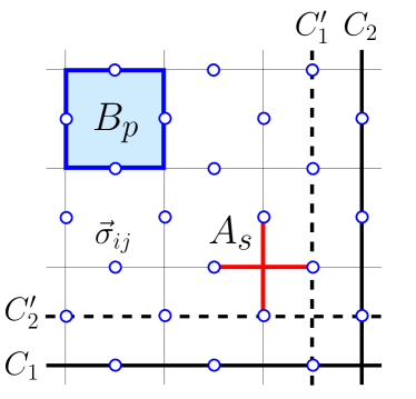
For the sake of clarity and because of historical importance we start by summarizing the main findings of Ref. NOLong regarding Kitaev’s Toric Code model kitaev in . The model is defined on a square lattice with sites, where on each bond (or link) it is defined a degree of freedom indicated by a Pauli matrix , thus defining a Hilbert space of dimension (see Fig. 1). The model Hamiltonian is given by
| (20) |
with Hermitian operators (whose eigenvalues are )
| (21) |
and () representing Pauli matrices. and describe the plaquette (or face) and star (or vertex) operators, respectively, with ()
| (22) |
thus generating an Abelian group called code’s stabilizer kitaev . In the presence of periodic boundary conditions, the plaquette and star operators satisfy the constraint
| (23) |
and the two symmetries are given by kitaev
| (24) |
where are horizontal and vertical closed contours (i.e. loops on the lattice(dual lattice)). The logical operators and commute with the code’s stabilizer but are not part of it, thus acting non-trivially on the two encoded Toric code qubits.
As shown in Ref. NOLong is related to Wen’s plaquette model wen_plaq and to two Ising chains by exact duality mappings. Therefore, these three models share the same spectrum. The GS (protected subspace of the code) is 4-fold degenerate (Abelian symmetry) and there is a gap to excitations. The spectrum is basically that of two uncoupled circular Ising chains ( is the total number of links of the original lattice)
| (25) |
with GS energy and a gap to the first excited state equals to 4 (this value of 4 and not 2 arises as in the presence of periodic boundary conditions, only an even number of domain walls are possible). This example clearly illustrates the fact that TQO is a property of states and not of the Hamiltonian spectrum NOLong .
The elementary excitations of are of two types kitaev
| (26) |
where is an open string on the lattice(dual lattice) and is a GS. (If would be closed contours which circumscribe an entire Toric cycle then the string operators would become the Toric symmetries of Eq. (24).) In the case of the open contours of Eq. (26), the operators generate excitations at the end points of these strings (thus always coming in pairs) with Abelian Fractional Statistics (anyons). Excitations living on the vertices represent electric charges while the ones living on the plaquettes are magnetic vortices. These magnetic and electric type excitations obey fusion rules that enable Abelian quantum computation. Due to the exact equivalence between Kitaev’s model and the Ising chains, no non-trivial finite temperature SSB or other transitions can take place. The spectrum exhibits a multitude of low-energy states. At any finite temperature, no matter how small, entropic contributions to the free energy overwhelm energy penalties and lead to a free energy which is everywhere analytic NOLong .
The operators of Eqs. (26) are not symmetries of and, for divergent loop size, are specific examples of the non-local operators that we considered earlier (see, e.g. Eq. (18)). In the one-dimensional Ising duality mapping of Eq. (25), we may represent the string operators of Eq. (26) as the creation operators for domain walls in the Ising model. When and intersect at any even number of bonds, a representation is
| (27) |
In Eq. (27), and denote the endpoints of the string of Eq. (26). Similarly, are the plaquettes which form the endpoints of the string on the dual lattice. When and share an odd number of bonds, we can represent the string operators as follows
| (28) |
For any finite lattice and
| (29) | |||||
where we have used the property and the cyclic invariance of the trace , which is performed over the eigenstates of with eigenvalues . Similarly, . Indeed, this is a special case of the more general argument depicted in Section II.
This does not, in principle, preclude SSB in the thermodynamic limit. One needs to restrict the configurations over which the trace is performed. In the thermodynamic limit, derivatives of the partition function and associated free energy need not be analytic single-valued functions (when SSB occurs the expectation values depend on how the limit is taken). To this end, let us define the (generating) partition function of the model with the constraint (23)
where . Thus, the free energy per bond, , is analytic for all finite , and displays a singularity at (inherited from the Ising chain). That means that no finite- phase transition occurs in Kitaev’s model. Moreover, from Eq. (III.1), we can compute the expectation values of the topological operators with the result
| (31) | |||||
This indicates that the existence of a gap in this system may not protect a finite expectation value of the Toric code operators or for any finite temperature NOLong ; alicki . At these expectation values are finite and equal to unity, reflecting the non-analyticity of at . The physical reason behind this result is the proliferation of topological defects (solitons) at any finite . The Boltzmann suppression becomes ineffective at sufficiently long times and this might be bad news for a robust quantum memory dennis . In the presence of additional fields (see last terms in Eq. (III.1)), with the two component vector at site , we may define the two component vector
| (32) |
and set ()
| (33) |
to be the counterparts of two single Ising spins and which are located at site numbers and of the two respective Ising chains (that of the and that of the varieties). and can be chosen to be any integers such that . These two spins (along with the spins appearing in Eq. (25) satisfy precisely the same algebra and set of constraints as the original variables in Kitaev’s model [Eqs. (20, 21, 24)]. The vanishing expectation values of Eq. (31) for both the finite and infinite system can be understood as the statement that for any one-dimensional Ising system when the single on-site magnetic fields .
The entropy associated with type domain walls is logarithmic in the system size . By contrast, the energy penalty for these domain walls is finite and size independent. As a result, for sufficiently large systems, entropic gains will outweigh energy penalties. In particular, in the thermodynamic limit, there is no SSB of the GLSs at any temperature . In NOLong , we showed how all static correlation functions may be computed via our mapping to the Ising chain.
We can now address the dynamical aspects of thermal fragility in Kitaev’s Toric code model. From its mapping to two uncoupled Ising chains, we can immediately determine the time autocorrelation functions of the Toric code operators. As we have shown, Kitaev’s Toric code operators map into single spins in an Ising chain. Thus, we can employ the results obtained in Glauber ; BP concerning autocorrelation of spins in Ising chains in a system with Glauber-type dynamics. In the Appendices (Eqs. (93, 94)), we will outline standard master equations which used to determine the dynamics. When these equations depend only on the system’s spectra (and not the precise real-space form of the GSs) then we can use our mapping of Eq. (33) to relate the dynamics of the non-local topological quantities of Kitaev’s Toric code model to single spin dynamics in Ising chains. We find that
| (34) |
obeys, for , the relation
| (35) |
Here, is a constant setting the time scale for the evolution of the system and is the modified Bessel function. For low temperatures, at short times, BP
| (36) |
the autocorrelation is given by
| (37) |
At intermediate times, BP
| (38) |
the autocorrelation of the topological string operators is well approximated by a Cole-Davidson form CD in the frequency domain and stretched exponential in time,
| (39) |
with the equilibration time
| (40) |
The constant is independent of the system size (for large systems) and is finite for all temperatures . If the temperature can be made much smaller than the gap, i.e. if , then , albeit being finite, can be made large (). We recall that in Kitaev’s Toric code model on the torus (the system with periodic boundary conditions) the gap between the GS and lowest excited energy levels is equal to four: [see the discussion after Eq. (25)]. (Similarly, the gap for the model on an open surface (open boundary conditions) is given by .) Thus, for Kitaev’s Toric code model on a torus, in the limit of small temperatures the inverse Botzmann factor scales in the same fashion as the equilibration time . The important feature of the scaling of the autocorrelation time in the Kitaev’s model is that, for large systems, it is system size independent at all temperatures. Similarly, in the long-time limit,
| (41) |
the autocorrelation function is well approximated by
| (42) | |||||
Identical relations hold for the autocorrelators . Thus, as we increase the system size the error rate will always be finite at any . In other words, any topological quantum memory at finite (non-zero) temperatures might not sustain self-correction indefinitely.
We now discuss Eq. (8). It is readily seen that this condition is violated here. For instance, if we choose , and with we have, for any finite , that
| (43) |
as . This is, of course, a particular realization of the general result of Appendix A. The Kitaev’s Toric code model has a transition and thus cannot satisfy the equilibrium thermal detection condition of Appendix A. It cannot be ruled out however that Kitaev’s Toric code model may nevertheless satisfy quantum error detection at finite temperature up to a small discrepancy nor that error detection may work well for finite time intervals.
On the other hand, by choosing , which has the property that
| (44) |
and realizing that the GS projection operator is given by
| (45) |
the detection condition, Eq. (4), is trivially satisfied. Similarly, if one chooses since
| (46) |
and, in general, for Kitaev’s model Eq. (4) is satisfied. That the conditions of Eq. (4) are satisfied also follows from the fact that Eq. (3) implies that Eq. (4), and as we proved in Ref. NOLong Kitaev’s model, satisfies the conditions of Eq. (3).
III.2 Generalizations of Kitaev’s Toric Code Model
There is obviously no connection between the lack of thermodynamic phase transition (as in Kitaev’s model) and the existence of TQO as defined in the Introduction. Indeed, we will now explore two models that have TQO yet display finite- phase transitions as signaled by non-analyticities in the free energy . The first model we will consider is a extension of Kitaev’s model and the second a gauge theory. In both of these systems, no SSB occurs (and TQO is indeed materialized). Nevertheless, the system’s free energy displays singularities at finite temperatures.
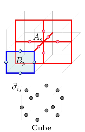
The Kitaev’s extended model (KE) in a cubic lattice has a Hamiltonian formally written as Eq. (20) with star (or vertex) operators , each comprising the 6 nearest-neighbors to a site, and planar plaquette operators , each involving 4 spins (see Fig. 2). This Hamiltonian is basically a Ising gauge theory () augmented by the sum of all local symmetry generators (). The constraints of Eq. (23) get replaced by
| (47) |
where Cube includes the six plaquettes which form the cube. Since no constraint couples the vertex and plaquette operators, the partition functions is simply
| (48) |
Let us first show that KE does show a thermodynamic phase transition at . From Eq. (48) the free energy is given by , where with the dual satisfying . Clearly, the free energy of KE displays a singularity coming from and a finite- singularity resulting from at .
We now show that the Ising Gauge theory displays (at least) rank TQO. [See the definition of rank- TQO given in the Introduction.] Let us start by writing 8 GSs of the Ising gauge theory on a cubic lattice of size which is endowed with periodic boundary conditions
| (49) |
In Eqs. (49), the states span all states in the basis which (i) have for each plaquette [see the definition of in Eq. (21)] and (ii) lie in a specific topological sector and is a uniform normalization constant. The eight topological sectors [] are labeled by three Toric invariants ()
| (50) |
Each of the eigenstates is an eigenstate of the three Toric operators . In Eq. (50), each of the three cycles is a path which circumscribes one Toric cycle (e.g. a cycle along each of the three cubic axes). Each of the states in Eq. (49) transforms as a singlet under all of the cubic lattice star operations
| (51) |
with the product above performed over all 6 bonds which have the vertex as one of their endpoints. This is so as the star operations of Eq. (51) link states within the same topological sector. That is, if
| (52) |
then, as for all and ,
| (53) |
Given the invariance of the 8 GSs of Eq. (49) [and thus of any superpositions thereof] under all of the symmetries , we may proceed to demonstrate TQO. To this end, let us decompose any quasi-local operator into the component invariant under all of the GLSs of Eq. (51) (labeled by ) and component which does not transform as a singlet under all of these operations: . For any state which lies in the 8-dimensional space spanned by the states of Eq. (49), and which transforms as a singlet under all GLSs , we have
| (54) |
All that we need to consider are thus the local () symmetry invariant components of the quasi-local operator . The quasi-local operators invariant under all of the symmetries of Eq. (51) are built out of product of a finite number of operators and plaquette operators (see Eq. (21)). We must now show that any such quasi-local operator attains the same expectation value in each of the states of Eq. (49). To this end, we consider the following three connecting operators
| (55) |
These operators are the extension of the operators of the gauge theory [Eq. (24)].
In Eq. (55), the product is taken over all bonds which lie in planes perpendicular to the cubic direction . These operators commute with one another and are symmetries of the Ising gauge Hamiltonian: . Acting with a particular on any state (e.g. any vortex-less eigenbasis state ) which is an eigenstate of all operators with unit eigenvalue leads to states which are eigenvectors of with unit eigenvalue. More generally, for any operators and , we have
| (56) |
As a consequence of Eq. (56) and the fact that all quasi-local operators are multinomials in , we have that
| (57) |
Moreover, these operators satisfy the following algebra with respect to the Toric symmetries :
| (58) |
As a consequence of Eq. (58), we see that the 8 states of Eq. (49) are related to one another by these operators. For instance,
| (59) |
etc.. Therefore, the 8 GLS operators with form a group (of a character). These operators suffice to link all of the states of Eq. (49) with one another. By unitarity, these generators also link any set of 8 orthogonal states in the space spanned by Eq. (49).
By Eqs. (54, 57), the expectation value of any quasi-local operator is the same in all GSs spanned by the GSs of Eq. (49). Thus, the Ising gauge theory exhibits (at least) rank- TQO.
We note, in passing, that considerations similar to those above may be enacted for general gauge theories () on a hypercubic -dimensional lattice. This theory is defined by
| (60) |
where, on every link , a parallel transporter
| (61) |
with an arbitrary integer. The elements of Eq. (61) satisfy a algebra. Here, instead of Eq. (55), we set
| (62) |
In Eq. (62), is the generator of rotation of the variable on bond . Replicating the proof given above, we find that the gauge theory on the -dimensional lattice exhibits (at least) rank- TQO.
It remains to prove that at any finite no topological symmetry operator may acquire a non-vanishing expectation value. For example,
| (63) |
for loops around the Toric cycles. [Equation (63) is a particular realization of Eq. (12).] Due to the decoupling of the plaquette ) and vertex () operators, the expectation value is given by its value for a classical Ising gauge theory. However, as seen by large and small coupling expansions kogut , the correlator vanishes in the Ising gauge theory as the bounding contours are taken to be infinite. [For finite size systems, vanishes as no SSB is possible.] In (i) the confined phase [] this correlator vanishes exponentially in the area of the minimal surface bounded by the Toric cycles while in (ii) the deconfined phase [], the pair correlator vanishes exponentially in the total length of the contours and . In the limit of far separated contours and , both (i) and (ii) reaffirm Eq. (63). Equation (63) is suggestive of a finite autocorrelation time at all positive temperatures.
III.3 Kitaev’s Honeycomb Model
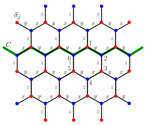
Kitaev’s model on the honeycomb lattice Kitaev2006 is defined by the following Hamiltonian (Fig. 3)
| (64) |
Here, we find that Elitzur’s theorem mandates that all non-vanishing expectation values must be of the form CN
| (65) |
with any contour (set of contours) drawn on the lattice and is the bond direction which is orthogonal to the path . Let us consider embedding this system on a torus with handles (a torus of genus ). For closed contours which do not span an entire Toric cycle, is not independent of the code’s stabilizer. In fact, there is a rather simple connection between these operators and the local anyon charge which measures the number of local high energy defects. For a closed contour which is an elementary closed hexagonal loop, we have which is the anyon charge associated with a given hexagon . Rather specifically,
| (66) |
with labeling the vertices of any given hexagon of Fig. 3. The spin polarization directions for all spins in the product of Eq. (66) have been chosen to correspond to the single bond direction ( or ) that is attached to the site and does not lie on the hexagonal path.
As shown by Kitaev, within the GS sector, for all . Extending the arguments of the strong and weak coupling expansions of gauge theories kogut , we now find that the correlator between any two contours scales as (i) at high temperatures with the area bounded by and and a positive constant and, if an ordered phase exists, scales at low temperatures as (ii) with the total perimeter of the two loops and another positive constant. Thus, for cycles which span the entire lattice we find as before that no loops of the form of Eq. (65) can attain a finite expectation value.
Let us now consider closed contours which span the same Toric cycle. For a system with periodic boundary conditions, at , we now have for closed contours ,
| (67) |
Here, is the domain bounded by two contours which go around an entire cycle of the torus [see e.g. the thick solid line in Fig. 3]. Taking the separation between the two contours and to be very large, we have that, at ,
| (68) |
This implies that, at ,
| (69) |
At , no SSB may occur (also in the thermodynamic limit, see Eq. (18)) and all quantities of the form Eq. (69) must be zero.
We now write down a formal finite temperature solution to the partition function and comment on low- and high- series expansions. Using fermionization CN , Kitaev’s Honeycomb model can be cast as a model for fermions on a square lattice with a site-dependent chemical potential .
| (70) | |||||
The fermionization of CN has been recently invoked to attain very interesting results in extensions of Kitaev’s Honeycomb model Yu . In Eq. (70), denote the centers of the vertical bonds. The unit vector connects two -bonds and crosses a -bond, see Fig. 3. A similar definition holds for CN . The form of Eq. (70) is very similar to the Fermi representation of the Ising model. In the last line of Eq. (70),
| (71) |
With Pan and
| (74) |
the partition function for the Fermi bilinear of Eq. (70) is easy to write down
| (75) |
Within the GS sector (the one with no anyons), the system is translationally invariant and its spectrum Kitaev2006 is that of a -wave type BCS pairing problem CN ; Yu .
Due to the sum over all of the Ising configurations , the complete partition function of Eq. (75) is non-trivial. The existence of a transition as temperature is varied is not as immediate as in Kitaev’s Toric code model. Translational invariance appears only for uniform or for all and by a simple unitary transformation to a system in which is constant on entire horizontal lines CN . Nevertheless, bounds on correlators are easily established: any fermionic correlator computed with the full partition function of Eq. (75) is bounded from above by its value when computed within the sector which maximizes its value. The finite fixed sector correlators for the quadratic Hamiltonian of Eq. (70) can be computed with the aid of Wick’s theorem. If the GS sector (that with everywhere) is gapped then at all temperatures, the correlation functions exhibit exponentially decaying correlations.
We may expand Eq. (75) in low- and high- series. A high- series may be derived by an expansion of in powers of . At low temperatures, the GS terms correspond to the phase for all which just reproduces the -wave type BCS result of Kitaev2006 ; CN . At finite temperatures, we allow for . The lowest energy terms correspond to a few vortex pairs () which are tightly bound. We may diagonalize the Hamiltonian to determine the spectrum for these vortex patterns and find the low- corrections to the GS results. In such a manner, we may write down a low- series expansion for the correlation function between fermion pairs (which corresponds to string correlators in terms of the spin variables of Kitaev’s model). The explicit high- and low- series expansions will be provided elsewhere. For now, let us note that within the gapped phase, the system exhibits a finite correlation length for these string correlators CN . It is clear that if a low- series expansion about the GSs is possible, then at sufficiently low temperatures, corrections to the result for the string correlators can be made arbitrarily small. In particular, when such an expansion is carried out about the GSs of the gapped phase, the string type correlators of BN still display a finite correlation length. [As we discussed above, that these string correlators must indeed display a finite correlation length also follows from the form of the fermionic correlator in the sector which maximizes its value; this value of the correlator provides an upper bound on the correlation function of the complete (unpinned ) system]. The correlation function on the righthand side of Eq. (69) is related to a limiting form of such string correlators in which the string (defined here by the contour ) wraps around an entire Toric cycle.
In what follows, we comment on the prospect of finite- phase transitions in Kitaev’s Honeycomb model as it follows from our expansions. As we show in the Appendix, in the absence of a phase transition, the topological quantum error detection condition of Eq. (8) [and its equivalent Eq. (81)], cannot be satisfied. If no transitions exist, then hardware fault-tolerance at finite temperatures may be impossible to achieve. The gapless phase - the phase which is not robust - seems to be amenable to a phase transition as the temperature of the system is increased. In the gapless phase, a transition from a system with oscillatory algebraic correlation between fermions at to one with exponential correlations at high temperatures is suggested by the low- and high- expansions. For states deep inside the gapless region Kitaev2006 ; CN a low- expansion (that includes sectors with a non-vanishing number of anyons) suggests that low-energy states may still carry a vanishing gap and lead to a phase with algebraic correlations. Thus, a finite- transition between a high- phase with exponentially decaying correlations between fermions to a low- stripe type phase with oscillatory algebraic correlations may exist.
In the absence of applied external fields which introduce a gap, the gapless sector of the theory is, however, unstable to perturbations. Of greater promise – insofar as stability to local perturbations – is the gapfull region of the Kitaev model. Regretfully, no transition of the type found for the gapless phase is evident for the gapfull sector of the Honeycomb model. Thus, albeit satisfying the condition of Eq. (4), in the absence of a finite- phase transition, the condition of Eq. (8) cannot be satisfied at any finite temperature.
Our results on the low- and high- expansions, which suggest that the gapfull sector of the Kitaev model does not exhibit a finite- phase transition, can be further fortified and linked to expansions carried by earlier works. These expansions elucidate how the gapfull phase will not break ergodicity and cannot achieve hardware fault-tolerance. The correspondence to our earlier results concerning Kitaev’s Toric code model is made clear by a simple mapping. In the parameter region , a perturbative expansion gives the following effective Hamiltonian Kitaev2006
| (76) |
In other words, we recover Kitaev’s Toric code model of Eq. (20). As a result, we have as before that the logical operators ( and ) have a finite (system-size independent) autocorrelation time [Eq. (39)].
IV Thermally stable orders in the case of high-dimensional broken symmetries - A case of simple non-TQO
Some systems with non-local symmetries exhibit a robustness to thermal fluctuations. These systems are natural contenders for satisfying the conditions of Eq. (8). In all of the cases that we examined, however, thermal fragility still appears.
Let us start with the simple orbital compass model. Its Hamiltonian is given by
| (77) |
which emulates the direction dependent interactions resulting from the anisotropy of electronic orbitals. In this model, exchange interactions involving the component of the spin occur only along the spatial -direction of the lattice. Similar spatial direction dependent spin exchange interactions appear for the components of the spin. Apart from a global reflection which only appears for the isotropic point (and which may be broken at low ), the anisotropic orbital compass model has the following symmetry operators for . denotes any line orthogonal to the axis. As involves sites, they constitute symmetries. The spectrum of the orbital compass model is gapless mila in the thermodynamic limit due to the existence of the symmetries that it possesses NOLong ; NF ; BN . What is important for relaxation processes (much as was evident in the analysis of Kitaev’s model) is not at all the energy spectrum but rather the free energy. It was found that the large renditions of the isotropic -dimensional orbital compass model, although highly degenerate in the low-energy spectra in the thermodynamic limit, exhibits free energy barriers. An entropic stabilization sets in which at sufficiently low yet finite leads to a sharp phase transition with a divergent relaxation time NBC . It is noteworthy, however, that at the isotropic point, the system is not topologically ordered as a global inversion symmetry
| (78) |
can be broken. It is this very symmetry which is broken below . Here, the local nematic order parameter operator
| (79) |
attains a finite expectation value at low NOLong ; NBC ; NF ; BN
| (80) |
Thus, measurements of this quasi-local order parameter within the GS sector lead to different answers for different contending low-energy Gibbs states (labeled by and ). Thus, is not a contending logical operator - it does not satisfy Eq. (10). For all non-local operators we have that at any finite , on any lattice (whether it is finite and no SSB is possible or on the infinite size lattice where the perimeter law scaling implies a vanishing ).
Similar arguments apply for the orbital compass model, meaning that the symmetries (as well as a three-dimensional reflection symmetry) will render the TQO non-existent at finite temperatures, although the relaxation time is obviously divergent. We recently became aware of a paper by Bacon bacon where he provides evidence (by using a mean-field approach) of a self-correcting system in a relative of the orbital compass model. The reason why this system is claimed to be a high-temperature self-correcting quantum memory (i.e. one without additional quantum error correction) is because, at the mean-field level, low-energy excitation energies may scale with the perimeter of the defected domain. As in the orbital compass model, Bacon’s model display (discrete) -GLSs. The problem we see with this argument is that these symmetries can be broken giving rise to an ordered phase (i.e. one with a Landau order parameter). Then, condition (3) is going to be violated and no TQO will be present. As in other cases in which symmetries can be broken, here Eq. (10) - a version of which is related to the weaker version [Eq. (9)] of the finite- error detection condition of Eq. (8) - will be violated.
V Can thermal fragility be defeated?
It is clear that a physical system that is in an ordered thermodynamic phase, i.e. having a non-vanishing Landau order parameter (i.e. breaking a global symmetry), displays some sort of robustness against local errors due to the collective nature of the resulting order. This property is used to build robust classical memories. We have seen that topological quantum memories seem to be thermally fragile, therefore, it seems plausible that by building systems that display an order parameter we could defeat it and obtain robust quantum memories. In general, there seems to be a catch regarding stable quantum topological memories. According to Eq. (8), in order to ensure error detection of local perturbations at finite temperatures, the system must display at least one finite temperature phase transition (see Appendix A). We generally find that . As a matter of principle, even if we allow for operators of a topological character (that is, non-local operators) which are not independent of the code’s stabilizer, unless a low- series expansion about the state is void, we will always get a perimeter-law type scaling for the quantum topological observables, see e.g. Eq. (18). This expansion for local Hamiltonians [see e.g. Ref. kogut ] always gives us the result that the topological observables vanish for large loops (for which local errors can be avoided at ). The expansion about can be void if there is a transition on an infinite size system. Such an occurrence matters worse once again as it implies that the robustness at does not obviously imply a robustness at any finite temperature (even at temperatures ). On any finite size system, there is no SSB and as before identically. We illustrated that the same also occurs in the thermodynamic limit of these systems. Ergodicity cannot be broken insofar as the logical operators can detect it.
We do not see an obvious way to avoid this conundrum both for the viable logical operators which are independent of the code’s stabilizer and more generally also for general non-local operators that can encode topological operations. It should be emphasized that all of our results pertain to rigorous bounds. Although finite (and size-independent) autocorrelation times seem to be mandated, if situations exist in which may be realized then the autocorrelation times can be made large (see e.g. the explicit form of Eq. (40)). Based on heuristics and static arguments, a recent review provides estimates on these ratios in some candidate systems ds .
VI Summary
In the present article we expanded on the concept of thermal fragility and applied it to several case examples including Kitaev’s Honeycomb model and extensions to higher spatial dimensions. Our main results are
(i) We introduced and discussed quantum error detection at finite temperature as it applies to topologically ordered systems [Eq. (8)].
(ii) We find that a system cannot satisfy the finite temperature error detection criteria of Eq. (8) unless it displays a finite temperature phase transition. It is important to emphasize that the existence of a finite temperature transition (or several finite temperature transitions) is a necessary but not sufficient condition for Eq. (8) to hold.
(iii) In general TQO systems, whether they display finite- phase transitions or not, and whether they have a finite size or are systems taken in the thermodynamic limit, all non-trivial topological operators may have a vanishing expectation value at all non-zero temperatures: . This suggests that the code might self-correct only up to finite cutoff times that are governed by temperature dependent effects. Depending on the relative size of the gaps to the temperature, this autocorrelation time can practically be made very large. This may go hand in hand with (system size independent) finite bounds on the autocorrelation times as adduced from the values of . For times , tends to zero [Eqs. (13, 39, 40, III.1)]. Information stored in the correlators of may be lost. Insofar as the non-local topological operators can detect, the system becomes ergodic at large time. Although of, apparently, less pertinence to ideal quantum memories, the same result is found for general operators which encode (non-local) topological operations on infinite-size systems but are not necessarily independent of the code’s stabilizer, Eq. (18), or correspond to symmetries.
(iv) Kitaev’s Toric code model can be solved exactly. At all non-zero temperatures, the autocorrelation function exhibits a finite equilibration beyond which ergodicity sets in and all information is lost. The explicit forms for the autocorrelation functions of Kitaev’s Toric code model are given in Eqs. (39, 40, III.1).
(v) Kitaev’s Honeycomb model can formally be solved at finite temperatures. The main utility of this formal solution is that it enables low- and high-temperature series expansions. These expansions suggest that this model may not be stable to thermal fluctuations (in the sense of Eq. (8)).
(vi) We showed that some candidate systems which are stable to thermal fluctuations often display local orders. These local orders render the system unstable to errors from local perturbations and the topological protection is lost.
A vexing question is how to quantify topological quantum error conditions at finite temperatures. The connection between rigorous bounds on quantum error detection and the more physical (although rigorous) results presented in our work is far from clear. In our opinion, this question needs to be quantitatively addressed. Given the physical results that we derived in our work, it is unclear to us if there is no way to overcome thermal fluctuations and still maintain quantum self-correction that is immune to local perturbations. We hope that our work will stimulate further studies which will address many related questions: Can GLSs lead to robust quantum memories? What is the relation between a finite lifetime and the vanishing expectation value of the logical operators ? What happens when a certain amount of disorder is present and thus, in general, -GLSs are not (exactly) present? In that case it is not true that for a finite system the expectation value of the logical operators vanishes since, for example for Kitaev’s Toric code model where represents the disorder. We conjecture that, nevertheless, in the thermodynamic limit those expectation values vanish, for example , and more importantly the autocorrelation times can generally remain finite as long as is an arbitrary quasi-local operator (and the amount of disorder is not big). Indeed, in our earlier work NOLong , we showed that system’s thermodynamic behavior and response functions may remain adiabatic even when their -GLSs may be broken.
The main message is that we need to be careful when designing a topological quantum memory. We are forced to consider finite temperature effects since a real system is subjected to temperature effects. The common lore that a finite gap can indefinitely protect states (and thus quantum information) is not always correct. The limiting size of the autocorrelation time can often be system independent. If very low temperatures may indeed be achieved relative to the gap ds then the autocorrelation time cutoff (e.g. Eq. (40)) can be made large (albeit still finite). It may also be that systems with a well crafted environment can be constructed; such environments will disallow rapid thermal equilibration and thus keep the autocorrelation times high. Possible realizations of such environments can include a frequency mismatch between the natural resonant frequencies of the TQO system and the environment in which it is embedded Loss .
In some of the Appendices that follow, we elaborate on points related to the main results reported here. In Appendix A, we prove that in the absence of a phase transition (a singularity in the free energy), the finite temperature error detection condition of Eq. (8) might not hold. In Appendix B, we discuss a trivial consequence of the Lieb-Robinson bounds to topological quantities. In Appendix C, we sketch how rigorous bounds for the excitation of anyons may be derived in some disorder free systems in thermal equilibrium. The derivation outlined here is intimately linked to Kitaev’s Honeycomb model of Section III.3. However, the result is far more general. In Appendix D, we discuss thermal equilibration time (the time for the system to become ergodic) in cases when the system displays or is close to a critical point and general scaling laws become apparent.
Note added in proof. After completing the current work and much after NOLong , we became aware of the interesting independent work of Ref. alicki which raised concerns about the reliable storage of quantum information at finite temperature. Reference alicki invoked the KMS equations in the study of Kitaev’s Toric code model to independently also arrive at and fortify one of the conclusions of Ref. NOLong (that of the last line of Eq. (31)) from a different approach.
Acknowledgements.
We thank the Perimeter Institute and the IQC for their hospitality. Manny Knill and John Preskill are acknowledged for helpful discussions. This work was sponsored, in part, by the CMI at Washington University, St. Louis (ZN).Appendix A Topological quantum error detection at finite temperatures
We show that any system that does not exhibit a finite temperature () phase transition (regardless of whether it exhibits TQO or not) necessarily violates the quantum error detection condition of Eq. (8) at all temperatures . In other words, for all
| (81) |
Here, we recall that with with the free energy. In the absence of a phase transition, the free energy may be expanded about its high temperature (small ) limit
| (82) |
All terms in the series of Eq. (82) are -numbers. If the system displays a phase transition the expansion of Eq. (82) has a finite radius of convergence (). If the system displays no phase transition, the series of Eq. (82) is everywhere convergent.
The proof of the assertion of Eq. (81) for the case a divergent (a system with no finite temperature transitions) is trivial. For any finite system at temperatures , the density matrix can be expanded to all orders in . We have that ()
| (83) |
At any fixed chosen for which is non-singular, the expansion of in powers of , with held at its fixed value at the chosen , has an infinite radius of convergence. In Eq. (83), we collect terms of a fixed power of when we use the expansion of Eq. (82). In the absence of a finite temperature phase transition, the series of Eq. (83) converges for all . If vanishes on a dense set of points along the real axis with arbitrary then as is an analytic function then it must also vanish everywhere in the complex -plane. All of the derivatives of and, in particular, its zeroth order value must vanish. However, is independent of the system in question (it is independent of , although ). For any non-trivial algebra captured by the operators , there exists quasi-local operators that (i) have their support on the same region where are defined, and (ii) do not commute with . Eq. (81) does not preclude a commutator which vanishes in the thermodynamic limit. The impossibility of Eq. (8) in the thermodynamic limit in all systems which exhibit SSB detectable by quasi-local operators follows from Eq. (9). In all finite size systems, there is no SSB (and the free energy is analytic - ) and Eq. (81) cannot be satisfied at any non-zero temperature. A similar conclusion holds for systems which, even in their thermodynamic limit, do not exhibit transitions. Kitaev’s Toric code model is precisely such a system. It is important to emphasize that the appearance of one (or more) transitions is a necessary but not sufficient condition for Eq. (8) to hold.
Appendix B Extensions of the Lieb-Robinson bound to non-local topological quantities
Locality in quantum spin systems is often well captured by a bound on the commutator of local observables with disjoint supports. Early on, Lieb and Robinson provided estimates and bounds on precisely such commutators on nearest-neighbor spin systems on general graphs. These naturally provide bounds for the speed of propagation of quantum information. Additional works elaborated on the initial findings of Lieb and Robinson and examined extensions to several bosonic and fermionic systems LR .
Stated formally, the Lieb-Robinson bound asserts that given two local operators and in different regions ( and ), the operator norm of the commutator in gapped systems
| (84) |
In Eq. (84), is the distance of the shortest path linking regions and (more precisely the number of links on such a path), denotes the number of vertices in the smaller of the two sets and . The constants and depend on the maximal coordination of a given vertex of the lattice and the largest local terms which appear in the argument of a nearest neighbor Hamiltonian system
| (85) |
Similar results are found to pertain to finite temperature correlators for systems with local Hamiltonians.
The extension of Eq. (84) to non-local quantities is straightforward. Let us consider the general product of local operators over an -dimensional volume
| (86) |
If the operator norm of all s is bounded from above by unity then the operator norm of the commutator
| (87) |
with and . In Eq. (87), denotes the smallest distance between two points - one which belongs in and the other in . The first line of Eq. (87) follows from a long-hand form of the expansion of the commutator. As contains terms and has terms, there are a total of terms each containing a string of length of local operators which bracket a single commutator between two local operators in the disjoint regions . If the operator norm of all s is bounded from above by unity then the bound of the last line of Eq. (87) follows from Eq. (84).
As , the equal time commutator between two distant topological operators vanishes. In some cases, the speed of propagation could be related to the velocity of defect motion (e.g. domain walls).
We can similarly bound the operator norm of the commutator which appears in Eq. (8). Here, we simply have that
| (88) |
Although the influence of events far away from the support of (region ) can become nil (as seen from Eq. (88), the cumulative effect of fluctuations on and proximate to can (and indeed generally does) lead to a vanishing .
Appendix C The probability of observing anyons
We now sketch how rigorous bounds on the probability of observing anyons may be derived in one of the models that we discussed in this work (Section III.3) - Kitaev’s Honeycomb model Kitaev2006 . Although some of the expressions given below are special, the result seems to be of greater applicability.
As shown by Kitaev, the GS configuration is the anyon-free configuration in which for all plaquettes (hexagons) . is the product of the two quantities which live on the center of two vertical bonds which appear in CN . As (i) this system exhibits reflection positivity (RP) RP for the Ising-type free energy () in the argument of Eq. (75),
| (89) |
(ii) the minimum of the spectrum of an slab of the system [of the square lattice of CN ] with open boundary conditions within a given topological sector is discrete, and as (iii) within the GS the system is anyon free, there must exist a length such that in all slabs of size the lowest free energy attainable over all states which are not anyon free is larger by a finite gap than the free energy within the anyon free infinite size system endowed with periodic boundary conditions. As, for example, in Ref. bcn and in particular zrp , this implies that the probability of finding anyons (or vortices in zrp ) is exponentially suppressed at sufficiently low temperatures. This is done by tiling the lattice with all blocks and noting that the probability for a given configuration is bounded from above by
| (90) |
where is a constant of order unity, is the number of bad blocks which contain (at least) one anyon and is the number of blocks to which a given bond is common. Combined with RP of the Ising-type Gibbs weight of Eq. (89), we can prove that the probability of anyons is exponentially damped in . Thus, although a gap is generally required for quantum protection from perturbations it may render the probability of excitations of such anyons exponentially small. Equation (90) is a rigorous result for any uniform RP system [including that of Eq. (64)]. It is noteworthy that the introduction of disorder may introduce anyons (and general defects) even at low temperatures. This has implications for impurities in Quantum Hall systems.
Appendix D Thermal Equilibration time in systems with discrete symmetries
We can use the following heuristic metastability argument to address the important question: How long does it take for a TQO system with -GLSs which has been prepared in the GS (protected subspace) to equilibrate at a temperature in the presence of -dimensional defects? Stated alternatively, we now address the following question: how long can the system retain information before it is lost due to ergodicity? The general answer to this question is quite complex. One can use qualitative ideas borrowed from the theory of metastable states, where the thermal equilibrium state is the global minimum of the free energy while the GS manifold is the suitable subspace which does not minimize but is supposed to be locally stable. The lifetime of the protected subspace is clearly determined by the dynamics of the system when coupled to a thermal reservoir. The basic problem then reduces to characterizing the free energy barrier that obstructs the escape from the GS manifold. The crucial observation is that for a system of size for a discrete symmetry of dimension , the free energy barrier follows the form
| (91) |
with a positive constant and the tension. The point is that the presence of low-dimensional symmetries lower the height of the barrier because of dimensional reduction. The case was considered in Section III (although the energy cost was finite in that case the entropy scaled logarithmically with the system size).
Let us assume that the probability to occupy an eigenstate of ,
| (92) |
with the initial state and a unitary evolution that includes the coupling to the thermal bath, follows a master equation
| (93) |
with transition probabilities satisfying the detailed balance condition (with equilibrium in a canonical ensemble)
| (94) |
It is clear that the whole complexity of the dynamical problem is in the functional form of the transition probabilities. Let us assume that there is only one possible channel for the system to escape from the local minima.
Kitaev’s model is quite special in that it displays a critical point. What can we say about systems that have a finite transition temperature?
Typically, in systems with a finite critical temperature, the equilibration time follows the Arrhenius form
| (95) |
with the free energy barrier for the defects. This, along with Eq. (91) leads to the usual form
| (96) |
In what follows, we address forms of this equilibration time and the surface tension which governs it in several regimes.
D.1 Equilibration time scaling near a critical point
The considerations presented below apply general scaling arguments (see e.g. glassme ) to general systems with discrete symmetries. For such systems, next to the critical point,
| (97) |
with the correlation length. Near the critical temperature the equilibration time scales as
| (98) |
with another positive constant. We can insert the scaling of with the reduced temperature near
| (99) |
to obtain the relaxation time near the critical point
| (100) |
D.1.1 Finite surface tension when
D.1.2 Temperature dependent surface tension
A temperature dependent surface tension may appear in the orbital compass model and other systems which exhibit an order-out-of-disorder phenomenon NBC ; bcn . Here, we can prove that at sufficiently low temperatures
| (101) |
This, then, enables the proof of a finite- phase transition by the usual Peierls argument. However, although the relaxation time is divergent in system size it does not, for a finite fixed , diverge as the temperature .
References
- (1) P. Shor, Proceedings of the Symposium on the Foundations of Computer Science, Los Alamitos, CA IEEE Press (1996).
- (2) A. Kitaev, Ann. Phys. 303, 2 (2003).
- (3) X-G. Wen, Quantum Field Theory of Many-Body Systems (Oxford University Press, Oxford, 2004), and references therein.
- (4) X-G. Wen, Phys. Rev. Lett. 90, 016803 (2003).
- (5) A. Yu. Kitaev, Ann. Phys. 321, 2 (2006).
- (6) Z. Nussinov and G. Ortiz, cond-mat/0605316 and cond-mat/0702377.
- (7) C. Castelnovo and C. Chamon, arXiv:0704.3616.
- (8) P.W. Anderson, Basic Notions of Condensed Matter Physics (Addison-Wesley, Redwood City, 1992).
- (9) F. Strocchi, Symmetry Breaking (Springer Verlag, Berlin, 2005).
- (10) In an SSB phase transition a Landau order parameter emerges at the transition. There are other type of phase transitions where there is no SSB of a global symmetry. However, in both cases, the existence of the phase transition is signaled by a non-analyticity of their free energies.
- (11) S. Elitzur, Phys. Rev. D 12 , 3978 (1975).
- (12) C. D. Batista and Z. Nussinov, Phys. Rev. B 72, 045137 (2005).
-
(13)
A working definition of the stabilizer of a code is the following. Let
be a subspace of an -qubit Hilbert space. The stabilizer of
is given by
Here, denote projection operators and is the projection operator onto the -qubit subspace .(102) - (14) E. Knill, private communication.
- (15) Wilson loops can be expressed as the products of the very same plaquette operators that appear in the lattice stabilizer codes that are generalizations of gauge theory Hamiltonians. [For instance, in the case of the Kitaev model which we will discuss in Section III.1, Wilson loops that circumscribe a region can be expressed where the operator of Eq. (21) was invoked.] Here, condition (i) applies. As such, in lattice gauge theory variants, the logical operators cannot be taken as Wilson loops and other general non-local operators .
- (16) J. B. Kogut, Rev. Mod. Phys. 51, 659 (1979).
-
(17)
If an expansion
about the (TQO) ordered state is void - if the system exhibits a
transition - then may vanish even
more rapidly as soon as temperature is made finite. The inequality of
Eq. (18) may be saturated (i.e. hold as an equality)
whenever an expansion about the ordered state is possible. If no
low- ordered state exists and no expansion about the state is
possible, then generally
with the size of the spatial support of even faster
then the ”perimeter law” bound of Eq.(18).
The simplest example is afforded by the two dimensional Ising
gauge theory kogut where for non-local
operators which are Wilson loops, the expectation
values do not fall off as Eq.(18) but
rather by, generally, a much faster decay. Here, unless
the spatial support of forms a closed loop,
identically by Elitzur’s theorem.
For spatial supports of that bound a given
”Area”,
we have that
where is a positive constant. In the two dimensional ) Ising gauge theory, an expansion about the state is void. Here, instead of Eq.(18), the much more dramatic fall-off of Eq.(103) always holds. As before, in the limit of an infinite spatial support of . Similarly, as we showed in NOLong , Kitaev’s Toric Code model exhibits a transition. In Kitaev’s Toric Code model an area law of the form of Eq.(103) holds at all positive temperatures. Here, once again, in the limit of an infinite spatial support of .(103) - (18) E.H. Lieb, D.W. Robinson, Commun. Math. Phys. 28, 251 (1972); B. Nachtergaele, and R. Sims, Commun. Math. Phys., 265, 119 (2006); B. Nachtergaele, Y. Ogata, and R. Sims, J. Stat. Phys. 124, 1 (2006); Jens Eisert and Tobias J. Osborne, Phys. Rev. Lett. 97, 150404 (2006); S. Bravyi, M. B. Hastings, and F. Verstraete, Phys. Rev. Lett. 97, 050401 (2006).
- (19) In lattice gauge theories in which such are realized, all Wilson loops kogut are invariant under all local (i.e. ) symmetries and may thus attain a finite expectation value at positive temperatures. However, as noted above Wilson loops are part of the code’s stabilizer. A Wilson loop is related to the product of all of the plaquette variables of all plaquettes inside the loop. Wilson loops and all local symmetries further commute with one another and do not realize the non-trivial algebra necessary for topological degeneracy: the operators are not Wilson loops. The absence of a SSB of detectable by any local measurement is the physical content of Eq. (10).
- (20) R. Alicki, M. Fannes, and M. Horodecki, quant-ph/0702102; J. Phys. A 40, 6451 (2007).
- (21) E. Dennis, A. Kitaev, A. Landahl, and J. Preskill, J. Math. Phys. 43, 4452 (2002).
- (22) R. J. Glauber, J. Math. Phys. 4, 294 (1963).
- (23) J. Javier Brey and A. Prados, Phys. Rev. E 53, 458 (1996).
- (24) D. W. Davidson and R. H. Cole, J. Chem. Phys. 19, 1484 (1951); D. W. Davidson and R. H. Cole, J. Chem. Phys. 18, 1417 (1950); K. S. Cole and R. H. Cole, J. Chem. Phys. 9, 341 (1941).
- (25) H-D. Chen and Z. Nussinov, cond-mat/0703633.
- (26) Y. Yu and Z. Wang, arXiv:0708.0631.
- (27) J-W. Pan et al., Phys. Rev. E 56, 2553 (1997).
- (28) J. Dorier, F. Becca, and F. Mila, Phys. Rev. B 72, 024448 (2005).
- (29) Z. Nussinov and E. Fradkin, Phys. Rev. B 71, 195120 (2005).
- (30) Z. Nussinov, M. Biskup, L. Chayes, and J. van den Brink, Europhysics Letters 67, 990-996 (2004); M. Biskup, L. Chayes, and S. Starr, Comm. Math. Phys. 269, 611 (2007).
- (31) D. Bacon, Phys. Rev. A 72, 012340 (2006).
- (32) S. Das Sarma, M. Freedman, C. Nayak, S. H. Simon, and A. Stern, arXiv:0707.1889, and references therein.
- (33) We are grateful to D. Loss for suggesting this possibility.
- (34) J. Frölich et al., Comm. Math. Phys. 62, 1 (1978).
- (35) M. Biskup, L. Chayes, and Z. Nussinov, Comm. Math. Phys. 255, 253 (2005).
- (36) Z. Nussinov, cond-mat/0107339.
- (37) D. Kivelson, S. A. Kivelson, X. L. Zhao, Z. Nussinov, and G. Tarjus, Physica A 219, 27 (1995); Z. Nussinov, Phys. Rev. B 69, 014208 (2004).