Non-relativistic limit in the 2+1 Dirac Oscillator: A Ramsey Interferometry Effect

Abstract

We study the non-relativistic limit of a paradigmatic model in Relativistic Quantum Mechanics, the two-dimensional Dirac oscillator. Remarkably, we find a novel kind of Zitterbewegung which persists in this non-relativistic regime, and leads to an observable deformation of the particle orbit. This effect can be interpreted in terms of a Ramsey Interferometric phenomenon, allowing an insightful connection between Relativistic Quantum Mechanics and Quantum Optics. Furthermore, subsequent corrections to the non-relativistic limit, which account for the usual spin-orbit Zitterbewegung, can be neatly understood in terms of a Mach-Zehnder interferometer.

I Introduction

The natural relativistic extension of the quantum harmonic oscillator, known as the Dirac oscillator moshinsky , has become a cornerstone in Relativistic Quantum Mechanics. It was initially introduced as a relativistic effective model to describe mesons, since it presents interesting quark-confinement properties ito ; cook . Moreover, subsequent studies have revealed several amazing properties of the Dirac oscillator in different contexts. Beyond its exact solvability, the energy spectrum presents certain peculiar degeneracies which can be related to a non-trivial symmetry Lie algebra moshinsky_lie . Furthermore, its solvability can be traced back to an exact Foldy-Wouthuysen transformation moreno , and its special properties are related to a hidden supersymmetry benitez_susy . Additionally, the positive- and negative-energy solutions are associated to supersymmetrical partners, which ensures the stability of the Dirac sea under the Dirac oscillator coupling matinez_romero_dirac_sea .

Some analogies between the dynamics of this relativistic model and the typical Jaynes-Cummings (JC) dynamics in Quantum Optics jaynes_cummings have been discussed in rozmej_1 , and some of its non-relativistic properties in rozmej_2 ; rozmej_3 ; rozmej_4 . Remarkably, in a two-dimensional setup this analogy becomes an exact equivalence between the 2+1 Dirac oscillator Hamiltonian and the Anti-Jaynes-Cummings (AJC) interaction wineland_review , which builds a bridge between two unrelated fields, Quantum Optics and Relativistic Quantum Mechanics, and favors a fruitful exchange of ideas between both communities bermudez_do_2D . Relativistic effects such as the Zitterbewegung, a helicoidal motion performed by the average position of a free relativistic fermion, can be reinterpreted with the language of Quantum Optics. This dynamical phenomenon also becomes observable in the spin and orbital degrees of freedom, where it can be surprisingly interpreted in terms of optical Rabi oscillations. In this work we shall be concerned with the extension of this novel perspective onto the non-relativistic limit of the two-dimensional Dirac oscillator. In this manner, we are able to identify a novel feature of the Zitterbewegung, which is interpreted as a Ramsey interferometry effect Ramsey . This remarkable effect shows that the standard non-relativistic limit described in Relativistic Quantum Mechanics textbooks should be reconsidered in this unusual scenario greiner .

This paper is organized as follows: in Sect. II, we review the properties of the two-dimensional Dirac oscillator and the exact mapping onto an AJC Hamiltonian. In Sect. III the non-relativistic limit is considered from a Quantum Optics perspective, which allows the prediction of a novel kind of Zitterbewegung which is interpreted as a Ramsey interferometric phenomenon in Sect. IV. In this section we also discuss how the effects of this interference process have strong consequences in the electron trajectory. In Sect. V, the analysis of additional corrections to the non-relativistic limit is discussed in terms of a Mach-Zehnder interferometer. There, we find that the first order non-trivial correction already shows a perturbative spin-orbit Zitterbewegung bermudez_do_2D . Finally, we conclude reviewing the consequences of our work in Sect.VI. In appendices A and  B we give detailed derivations of the standard non-relativistic limit and its complete perturbative series, respectively.

II Two-dimensional Dirac Oscillator

The physical laws that describe the properties of microscopic particles are accurately described by Quantum Mechanics, and in particular by the Schrödinger equation. Nonetheless, quantum phenomena occurring at high energies cannot be properly addressed by such theory, and one must employ Relativistic Quantum Mechanics greiner . A relativistic spin-1/2 particle of mass $m$ is described by the Dirac equation

$${\rm i}\hbar\frac{\partial|\Psi\rangle}{\partial t}=\left[c\bm{\alpha}\cdot\textbf{p}+\beta mc^{2}\right]|\Psi\rangle,$$ (1)

where $|\Psi\rangle$ is the four-component Dirac spinor, $\alpha_{i}:=\text{off-diag}(\sigma_{i},\sigma_{i})$ , and $\beta:=\text{diag}(\mathbb{I}_{2},-\mathbb{I}_{2})$ are known as the Dirac matrices which can be expressed in terms of the usual Pauli matrices $\sigma_{i}$, p is the momentum operator, and $c$ stands for the speed of light.

The Dirac oscillator is obtained after the introduction of a peculiar coupling in the above equation (1)

$${\rm i}\hbar\frac{\partial|\Psi\rangle}{\partial t}=\left[c\bm{\alpha}\cdot\left(\textbf{p}-{\rm i}m\beta\omega\textbf{r}\right)+\beta mc^{2}\right]|\Psi\rangle,$$ (2)

where $\omega$ stands for the Dirac oscillator frequency, and r represents the particle position. The relativistic coupling $\textbf{p}-{\rm i}m\beta\omega\textbf{r}$, known as a Dirac string, cannot be understood as a simple minimal coupling procedure, and is responsible for the special properties of this relativistic system. In particular, the non-relativistic limit of the aforementioned Dirac oscillator (2) leads to the usual non-relativistic harmonic oscillator with an additional spin-orbit coupling which shows the intrinsic spin structure of the relativistic theory moshinsky .

The restriction to two-spatial dimensions appreciably simplifies the relativistic problem, since the Dirac matrices become $2\times 2$ matrices which can be identified with the so-called Pauli matrices $\alpha_{x}=\sigma_{x},\alpha_{y}=\sigma_{y},\beta=\sigma_{z}$. In this manner, $|\Psi\rangle$ can be described by a 2-component spinor, and the Dirac oscillator model now takes the form

$${\rm i}\hbar\frac{\partial|\Psi\rangle}{\partial t}=\left[\sum_{j=1}^{2}c\sigma_{j}\left(p^{j}-{\rm i}m\sigma_{z}\omega r^{j}\right)+\sigma_{z}mc^{2}\right]|\Psi\rangle.$$ (3)

This two-dimensional system was algebraically solved bermudez_do_2D by introducing chiral creation and annihilation operators

$$\begin{array}[]{c}a_{r}:=\frac{1}{\sqrt{2}}(a_{x}-{\rm i}a_{y}),\hskip 8.61108pta_{r}^{\dagger}:=\frac{1}{\sqrt{2}}(a_{x}^{\dagger}+{\rm i}a_{y}^{\dagger}),\\ a_{l}:=\frac{1}{\sqrt{2}}(a_{x}+{\rm i}a_{y}),\hskip 8.61108pta_{l}^{\dagger}:=\frac{1}{\sqrt{2}}(a_{x}^{\dagger}-{\rm i}a_{y}^{\dagger}),\\ \end{array}$$ (4)

where $a_{x},a_{x}^{\dagger},a_{y},a_{y}^{\dagger}$, are the usual annihilation-creation operators $a^{\dagger}_{j}=\frac{1}{\sqrt{2}}\left(\frac{1}{\Delta}r^{j}-{\rm i}\frac{\Delta}{\hbar}p^{j}\right)$, and $\Delta=\sqrt{\hbar/m\omega}$ represents the ground state oscillator width. These operators allow an insightful derivation of the energy spectrum

$$E=\pm E_{n_{l}}=\pm mc^{2}\sqrt{1+4\xi n_{l}},$$ (5)

where the integer $n_{l}$ stands for the number of left-handed orbital quanta, and $\xi:=\hbar\omega/mc^{2}$ is an important parameter that specifies the importance of relativistic effects in the Dirac oscillator. A different approach, based on the solution of differential equations, has also been discussed in villalba .The associated eigenstates are found to be

$$\begin{array}[]{c}|+E_{n_{l}}\rangle=\alpha_{n_{l}}|n_{l}\rangle|\chi_{\uparrow}\rangle-{\rm i}\beta_{n_{l}}|n_{l}-1\rangle|\chi_{\downarrow}\rangle,\\ |-E_{n_{l}}\rangle=\beta_{n_{l}}|n_{l}\rangle|\chi_{\uparrow}\rangle+{\rm i}\alpha_{n_{l}}|n_{l}-1\rangle|\chi_{\downarrow}\rangle,\\ \end{array}$$ (6)

where $|\chi_{\uparrow}\rangle:=(1,0)^{t}$ and $|\chi_{\downarrow}\rangle:=(0,1)^{t}$ are known as the Pauli spinors, and $\alpha_{n_{l}}:=\sqrt{(E_{n_{l}}+mc^{2})/2E_{n_{l}}}$ and $\beta_{n_{l}}:=\sqrt{(E_{n_{l}}-mc^{2})/2E_{n_{l}}}$ are real normalization constants.

The notation in Eq. (6) clearly shows that the relativistic eigenstates exhibit entanglement between the orbital and spin degrees of freedom. This entanglement property is essential in order to obtain the relativistic effect of spin-orbit Zitterbewegung, where certain oscillations in the orbital and spin angular momentum are unambiguously identified with the interference of positive- and negative-energy components. Introducing the spin and angular momentum operators $S_{z}=\textstyle\frac{1}{2}\hbar\sigma_{z}$ and $L_{z}=\hbar(a^{\dagger}_{r}a_{r}-a^{\dagger}_{l}a_{l})$, and considering the initial state $|\Psi(0)\rangle:=|n_{l}-1\rangle|\chi_{\downarrow}\rangle$, one immediately finds the so-called spin-orbit oscillations associated to the Zitterbewegung

$$\begin{array}[]{l}\langle L_{z}\rangle_{t}=-\frac{4\xi n_{l}}{1+4\xi n_{l}}\hbar\sin^{2}\omega_{n_{l}}t-\hbar(n_{l}-1),\\ \langle S_{z}\rangle_{t}=\hskip 8.61108pt\frac{4\xi n_{l}}{1+4\xi n_{l}}\hbar\sin^{2}\omega_{n_{l}}t-\frac{\hbar}{2},\\ \langle J_{z}\rangle_{t}=\hskip 8.61108pt\hbar(\textstyle\frac{1}{2}-n_{l}),\end{array}$$ (7)

where $J_{z}=L_{z}+S_{z}$ stands for the $z$-component of the total angular momentum and is obviously a conserved quantity.

Finally, we recall the interesting mapping between the two-dimensional Dirac oscillator and the AJC model bermudez_do_2D , where the relativistic hamiltonian can be written as

$$\begin{split}H&=\hbar(g\sigma^{+}a_{l}^{\dagger}+g^{*}\sigma^{-}a_{l})+\delta\sigma_{z},\end{split}$$ (8)

with $\sigma^{+}:=|\chi_{\uparrow}\rangle\langle\chi_{\downarrow}|$, $\sigma^{-}:=|\chi_{\downarrow}\rangle\langle\chi_{\uparrow}|$ as the spin raising and lowering operators, $g:=2{\rm i}mc^{2}\sqrt{\xi}/\hbar$ as the coupling strength between orbital and spin degrees of freedom, and where $\delta:=mc^{2}$ can be interpreted as a detuning parameter. In Quantum Optics, this Hamiltonian describes an Anti-Jaynes-Cummings interaction, and can be implemented with trapped ions wineland_review . Within this novel perspective, the electron spin can be associated with a two-level atom, and the orbital circular quanta with the ion quanta of vibration, i.e., phonons. Note that there is also the possibility to map this relativistic Hamiltonian onto the more standard Jaynes-Cummings model comment1 . In the following section, we derive the non-relativistic limit of the two-dimensional Dirac oscillator (8), and discuss the nature of the physical properties described in Eqs. (5)-(7) in this non-relativistic scenario.

III Non-relativistic limit in Quantum Optics

The original Quantum Optics perspective of the two-dimensional Dirac oscillator in Eq. (8) stimulates the use of quantum optical tools in a relativistic quantum framework, and viceversa. In particular, we can use the quasi-degenerate perturbation theory cohen in order to derive an effective Hamiltonian in the non-relativistic limit. This regime is attained when the relativistic parameter fulfills $\xi n_{l}\ll 1$, which allows the usual description of the Dirac oscillator Hamiltonian in Eq. (8)

$$H=H_{0}+\lambda V,$$ (9)

where $H_{0}$ is the unperturbed Hamiltonian

$$H_{0}=\delta\sigma_{z},$$ (10)

and $\lambda V$ represents the following perturbation

$$\lambda V=\lambda(\sigma^{+}a_{l}^{\dagger}-\sigma^{-}a_{l}),$$ (11)

where the interaction coupling $\lambda:=2{\rm i}mc^{2}\sqrt{\xi}$ satisfies $|\lambda|\ll\delta$, and consequently the coupling in Eq. (11) can be treated as a small perturbation. In this regime, the Hilbert space can be divided into two approximately disconnected subspaces

$$\mathcal{H}\approx\mathcal{H}_{\uparrow}\oplus\mathcal{H}_{\downarrow},$$ (12)

where

$$\begin{split}\mathcal{H}_{\uparrow}=\text{span}\{|n_{l}\rangle|\chi_{\uparrow}\rangle;n_{l}=0,1...\},\\ \mathcal{H}_{\downarrow}=\text{span}\{|n_{l}\rangle|\chi_{\downarrow}\rangle;n_{l}=0,1...\}.\end{split}$$ (13)

This is easily understood from the fact that $\xi n_{l}\ll 1$ is equivalent to $\hbar\omega\ll\delta$, which implies that the perturbation in Eq. (11) does not suffice to induce transitions between the spinor components. In this manner, the subspaces corresponding to the spinor degrees of freedom become decoupled, and we may describe the effective dynamics in such subspaces ( see fig. 1 ).

\begin{overpic}[width=241.84842pt]{couplings_scheme_pra.eps} \par\put(16.0,38.0){{\color[rgb]{0.37,0.00,0.00}\large{$\mathcal{H}_{\uparrow}$}}} \put(78.0,38.0){{\color[rgb]{0.00,0.21,0.00}\large{$\mathcal{H}_{\downarrow}$}}} \put(10.0,50.0){$|\psi_{\uparrow}\rangle$}\put(22.0,50.0){$|\psi^{\prime}_{\uparrow}\rangle$} \put(71.0,49.0){$|\psi_{\downarrow}\rangle$}\put(84.0,49.0){$|\psi^{\prime}_{\downarrow}\rangle$} \put(45.0,5.0){$|\lambda|\ll\delta$} \put(17.0,66.0){$H_{\text{eff}}^{\uparrow}$} \put(78.0,66.0){$H_{\text{eff}}^{\downarrow}$} \end{overpic}

Figure 1: ”(Color online)” Schematic diagram of the Dirac oscillator couplings in the non-relativistic limit. The subspaces $\mathcal{H}_{\uparrow}$ and $\mathcal{H}_{\downarrow}$ become disconnected in this regime

In order to obtain the effective Hamiltonian, we rewrite the perturbation in Eq. (11) as follows

$$\lambda V=\sum_{\mu}\lambda_{\mu}A_{\mu}B_{\mu},$$ (14)

where $\mu=1,2$, the operators $A_{1}=a_{l},A_{2}=a^{\dagger}_{l}$ describe the slow varying orbital degrees of freedom, whereas the operators $B_{1}=\sigma^{-},B_{2}=\sigma^{+}$ represent the coupling of the fast spinorial degrees of freedom, and $\lambda_{1}=g,\lambda_{2}=g^{*}$. The effective Hamiltonians correspond to

$$\begin{split}H_{\text{eff}}^{\uparrow}&=\hskip 8.61108pt\delta+\sum_{\mu\mu^{\prime}}\langle\chi_{\uparrow}|\lambda_{\mu}B_{\mu}\frac{1}{\delta-H_{0}}\lambda_{\mu^{\prime}}B_{\mu^{\prime}}|\chi_{\uparrow}\rangle A_{\mu}A_{\mu^{\prime}},\\ H_{\text{eff}}^{\downarrow}&=-\delta+\sum_{\mu\mu^{\prime}}\langle\chi_{\downarrow}|\lambda_{\mu}B_{\mu}\frac{1}{\delta-H_{0}}\lambda_{\mu^{\prime}}B_{\mu^{\prime}}|\chi_{\downarrow}\rangle A_{\mu}A_{\mu^{\prime}},\end{split}$$ (15)

which can be readily evaluated as

$$H_{\text{eff}}=\left[\begin{array}[]{cc}mc^{2}+2\hbar\omega a_{l}^{\dagger}a_{l}&0\\ 0&-mc^{2}-2\hbar\omega a_{l}a_{l}^{\dagger}\\ \end{array}\right].$$ (16)

The effect of the relativistic corrections in this regime can be understood as a level shift with respect to the rest mass energy that depends on the number of left-handed quanta. The non-relativistic energies associated to the corresponding eigenstates $|n_{l}\rangle|\chi_{\uparrow}\rangle$ and $|n_{l}-1\rangle|\chi_{\downarrow}\rangle$ are

$$\begin{split}E_{|n_{l}\rangle|\chi_{\uparrow}\rangle}&=+mc^{2}(1+2\xi n_{l}),\\ E_{|n_{l}-1\rangle|\chi_{\downarrow}\rangle}&=-mc^{2}(1+2\xi n_{l}),\end{split}$$ (17)

which are equivalent to the leading order correction of the exact eigenvalues (5) in the limit $\xi n_{l}\ll 1$, namely,

$$E=\pm mc^{2}\sqrt{1+4\xi n_{l}}\approx\pm mc^{2}(1+2\xi n_{l})+\mathcal{O}\left((\xi n_{l})^{2}\right).$$ (18)

Therefore, we obtain the so-called energy shift term $\Delta E=2mc^{2}(1+2\xi n_{l})$ , which is usually known as a dynamical Stark shift term in the quantum optics literature Stark . In Optics, the non-relativistic effective Hamiltonian (16) achieved for large enough detuning is equivalent to the dispersive linear susceptibility and the real part of the refraction index, with opposite contributions from the excited and ground states SI86 .

This noteworthy interpretation of the non-relativistic limit in terms of measurable optical quantities is shown to be equivalent to the standard non-relativistic limit in Relativistic Quantum Mechanics in Appendix A. In the following section, we shall use this remarkable perspective to describe a novel sign of the Zitterbewegung, which can be understood in terms of a Ramsey interferometry effect Ramsey .

IV Zitterbewegung in the non-relativistic limit

As discussed in previous sections, the interference between positive- and negative-energy components gives rise to a relativistic oscillatory behavior known as Zitterbewegung. This phenomenon has a pure relativistic nature, and therefore it is usually believed to vanish in the non-relativistic limit. Contrary to common belief, we show in this section how a peculiar Zitterbewegung effect can still arise in the non-relativistic regime if the initial state is appropriately prepared. Furthermore, we also discuss how this dynamics might be interpreted as a Ramsey interferometry phenomenon, and how it can lead to measurable effects in the particle trajectory.

Let us consider an initial state $|\Psi(0)\rangle:=\alpha|n_{l}\rangle|\chi_{\uparrow}\rangle+\beta|n_{l}-1\rangle|\chi_{\downarrow}\rangle$, which involves both spinorial components, where $\alpha,\beta\in\mathbb{C}$ are correctly normalized $|\alpha|^{2}+|\beta|^{2}=1$. One directly observes that this state mixes the positive- and negative-energy solutions in Eq. (17), which is the fundamental ingredient leading to the Zitterbewegung. In order to obtain such effect, we derive the time evolution under the effective Hamiltonian (16)

$$|\Psi(t)\rangle=\alpha e^{-{\rm i}\Omega_{n_{l}}t}|n_{l}\rangle|\chi_{\uparrow}\rangle+\beta e^{+{\rm i}\Omega_{n_{l}}t}|n_{l}-1\rangle|\chi_{\downarrow}\rangle,$$ (19)

where $\Omega_{n_{l}}:=mc^{2}(1+2\xi n_{l})/\hbar$. The corresponding spin-orbit expected values (7) become

$$\begin{array}[]{l}\langle L_{z}\rangle_{t}=-\hbar\left(n_{l}+|\beta|^{2}\right),\\ \langle S_{z}\rangle_{t}=\frac{\hbar}{2}\left(|\alpha|^{2}-|\beta|^{2}\right),\\ \langle J_{z}\rangle_{t}=\frac{\hbar}{2}\left(2n_{l}+|\alpha|^{2}-3|\beta|^{2}\right),\end{array}$$ (20)

where any remainder of the original oscillatory Zitterbewegung in Eq. (7) has completely vanished. Nevertheless, positive- and negative-energy components are simultaneously involved in the initial state, and therefore there must exist some kind of novel Zitterbewegung.

The possibility to observe such effect can be achieved if we consider the superposition of states with different energy modulus $|E_{n_{l}}|$. This novel Zitterbewegung can be exemplified by a Ramsey interferometer in which the field is prepared in a coherent state and the atom in a 50 % superposition of its excited and ground states ( i.e. $\alpha|\chi_{\uparrow}\rangle+\beta|\chi_{\downarrow}\rangle$) by resonant interaction with a classical laser beam Ramsey . Afterwards, the effective interaction produces a different field evolution conditioned to the atomic level. Finally, resonant interaction of the atom with a second laser beam mixes the contributions from the upper and lower levels leading to the interference of the positive- and negative-energy evolutions. Therefore, the Ramsey fringes such as the ones in Refs. RF can be regarded as suitable examples of Zitterbewegung in this particular regime.

Let us exemplify this Ramsey-Zitterbewegung with the following initial state prepared in a superposition of the two-spinor states $|\Psi(0)\rangle:=|z_{l}\rangle(\alpha|\chi_{\uparrow}\rangle+\beta|\chi_{\downarrow}\rangle)$, where $|z_{l}\rangle:={\rm e}^{-|z_{l}|^{2}/2}\sum_{n_{l}}z_{l}^{n_{l}}|n_{l}\rangle/\sqrt{n_{l}!}$ represents a left-handed coherent state with $z_{l}\in\mathbb{C}$. This initial state also involves positive- and negative-energy components, and its time evolution is

$$|\Psi(t)\rangle=\alpha{\rm e}^{-{\rm i}\Omega_{0}t}|z_{l}{\rm e}^{-2{\rm i}\omega t}\rangle|\chi_{\uparrow}\rangle+\beta{\rm e}^{+{\rm i}\Omega_{1}t}|z_{l}{\rm e}^{+2{\rm i}\omega t}\rangle|\chi_{\downarrow}\rangle.$$ (21)

As time elapses, the phase evolution of the orbital coherent state is strongly correlated to the internal spinorial degree of freedom, just as the Ramsey interferometric time evolution. This peculiar correlated dynamics is a clear consequence of the coexistence of positive- and negative-energy modes in the initial state, and therefore it stands as a direct symptom of Zitterbewegung. The final step in the Ramsey interferometric experiment is to recombine both spinor components leading to the interference of positive- and negative-energy modes. The measurement of $S_{z}$ after this mixing effect is equivalent to the measurement of the $x$-component of the spin angular momentum $S_{x}:=\frac{\hbar}{2}\sigma_{x}$ in the state (21)

$$\langle S_{x}\rangle_{t}=\hbar\mathcal{V}(t)\cos\left[(\Omega_{0}+\Omega_{1})t+|z_{l}|^{2}\sin(4\omega t)+\text{arg}({\alpha^{*}\beta})\right]$$ (22)

where $\mathcal{V}(t)=|\alpha^{*}\beta|{\rm e}^{-2|z_{l}|^{2}\sin(2\omega t)}$ can be identified with a periodic visibility factor which precedes the desired Ramsey interference term. Therefore, an oscillatory behaviour in the $x-$spin component can be directly traced back to a Zitterbewegung in the non-relativistic limit. Note that this phenomenon is consequence of an appropriate preparation of the initial state, involving both energy modes, rather than the pure dynamical effect in Eqs. (7).

This Ramsey interferometric dynamics (21) can lead to measurable effects in the electron trajectory, since the interference of both energy modes undeniably causes a deformation of the particle orbit. The electron trajectory is described by the following position operators $x=\Delta(a_{r}+a_{r}^{\dagger}+a_{l}+a_{l}^{\dagger})/2$, $y={\rm i}\Delta(a_{r}-a_{r}^{\dagger}-a_{l}+a_{l}^{\dagger})/2$, whose expectation values evolve according to

$$\begin{split}\langle x\rangle_{t}&=\Delta|z_{l}|\left[|\alpha|^{2}\cos(2\omega t-\phi_{l})+|\beta|^{2}\cos(2\omega t+\phi_{l})\right],\\ \langle y\rangle_{t}&=\Delta|z_{l}|\left[|\beta|^{2}\hskip 0.86108pt\sin(2\omega t+\phi_{l})-|\alpha|^{2}\hskip 0.86108pt\sin(2\omega t-\phi_{l})\right],\end{split}$$ (23)

where we have used $z_{l}=|z_{l}|{\rm e}^{{\rm i}\phi_{l}}$. The particle trajectory described in Eq. (23) has a remarkable periodic character, and must be compared to the Zitterbewegung-free trajectory of an initial state $|\Psi(0)\rangle:=|z_{l}\rangle|\chi_{\uparrow}\rangle$, which is described by a circular orbit

$$\begin{split}\langle x\rangle_{t}&=+\Delta|z_{l}|\cos(2\omega t-\phi_{l}),\\ \langle y\rangle_{t}&=-\Delta|z_{l}|\hskip 0.86108pt\sin(2\omega t-\phi_{l}).\end{split}$$ (24)

Comparing both trajectories in Eqs. (23),(24), we realize that the Zitterbewegung phenomenon leads to a deformation of the electron circular orbit (24) ( see fig. 2)

\begin{overpic}[width=241.84842pt]{NR_trajectories_pra.eps} \put(45.0,3.0){$\langle x\rangle/|z_{l}|^{2}$} \put(-5.0,45.0){$\langle y\rangle/|z_{l}|^{2}$} \put(73.0,21.0){{\color[rgb]{0.00,0.21,0.00}$\small{\alpha_{1}}$}} \put(65.0,28.0){{\color[rgb]{0.41,0.70,0.13}$\small{\alpha_{2}}$}} \put(51.0,38.0){{\color[rgb]{0.50,0.50,0.00}$\small{\alpha_{3}}$}} \end{overpic}

Figure 2: ”(Color online)” Electron trajectory for different initial states where the coherent state phase is $\phi_{l}=\pi/2$, and $\alpha_{i}=\{1,\sqrt{2/3},\sqrt{1/2}\}$, with $i=1,2,3$. Note that $\alpha_{1}=1$ corresponds to the circular Zitterbewegung-free evolution in Eq. (24), as compared to the elliptic orbits caused by a Zitterbewegung interference.

In light of the results presented in this section, we may conclude that Zitterbewegung phenomena may also arise in a non-relativistic regime as long as the initial state involves both energy modes, which is still a relativistic property. The initial state, which can be described by a coherent superposition of positive- and negative-energy solutions, cannot be described in the realm of non-relativistic quantum mechanics. Therefore, the persistence of Zitterbewegung in the non-relativistic regime can be traced back to the relativistic nature of the initial state, when carefully prepared.

Furthermore, we have also described how this interference effect can be unexpectedly interpreted in terms of Ramsey fringes in the context of Quantum Optics. The effect of this relativistic interference can be observed in oscillations in the $x-$spin component, or even more drastically in the deformation of the electron circular orbit into an elliptic trajectory.

V Corrections to the non-relativistic limit

In section III we have discussed the non-relativistic limit of the two-dimensional Dirac oscillator, where the decoupling of the spinor components leads to a dynamical Stark shift in the energy levels. It was precisely this energy shift, which allowed the surprising description of the Zitterbewegung in terms of a Ramsey interferometry effect in Sect. IV. In the present section, we consider how relativistic effects modify such picture as the parameter $\xi$ increases, and interpret the usual spin-orbit Zitterbewegung described in Eqs. (7) as a first order perturbation term. The picture developed in section III is no longer valid, since it assumes the decoupling of the spinor subspaces (13), which forbids this peculiar dynamics. Therefore, we discuss a novel description which allows the interpretation of the spin-orbit Zitterbewegung in terms of a Mach-Zehnder interferometer.

Let us consider the AJC-mapping of the two-dimensional Dirac oscillator (8), which allows the description of the Hilbert space as a series of invariant subspaces $\mathcal{H}=\bigoplus_{n_{l}=1}^{\infty}\mathcal{H}_{n_{l}}$, where

$$\mathcal{H}_{n_{l}}=\text{span}\{|n_{l}\rangle|\chi_{\uparrow}\rangle,|n_{l}-1\rangle|\chi_{\downarrow}\rangle\}.$$ (25)

The relativistic Hamiltonian in these subspaces reads

$$H_{n_{l}}=mc^{2}\left(\sigma_{z}-\eta_{n_{l}}\sigma_{y}\right),$$ (26)

where we have introduced a parameter $\eta_{n_{l}}=2\sqrt{\xi n_{l}}$ directly related to the small relativistic parameter $\xi n_{l}\ll 1$. This interaction can be considered as a rotation of the $\sigma_{z}$ term along the $x$-axis

$$H_{n_{l}}=mc^{2}\sqrt{1+\eta_{n_{l}}^{2}}{\rm e}^{-{\rm i}\theta_{n_{l}}\sigma_{x}}\sigma_{z}{\rm e}^{{\rm i}\theta_{n_{l}}\sigma_{x}},$$ (27)

where the rotation angle satisfies $\tan(2\theta_{n_{l}}):=\eta_{n_{l}}$ KS00 . The unitary time evolution operator can be expressed as follows

$$U_{n_{l}}={\rm e}^{-\frac{{\rm i}t}{\hbar}H_{n_{l}}}={\rm e}^{-{\rm i}\theta_{n_{l}}\sigma_{x}}{\rm e}^{-{\rm i}\phi_{n_{l}}(t)\sigma_{z}}{\rm e}^{{\rm i}\theta_{n_{l}}\sigma_{x}},$$ (28)

where

$$\phi_{n_{l}}(t)=\frac{mc^{2}}{\hbar}\sqrt{1+\eta_{n_{l}}^{2}}t.$$ (29)

This evolution has a clear interferometric interpretation in terms of a Mach-Zehnder interferometer ( see fig. 3).

\begin{overpic}[width=227.62204pt]{mach-zender_bis_pra.eps} \put(24.0,30.0){{\color[rgb]{0.00,0.00,0.35}$\theta_{n_{l}}$}} \put(70.0,71.0){{\color[rgb]{0.00,0.00,0.35}$-\theta_{n_{l}}$}} \put(3.0,38.0){$|n_{l}\rangle|\chi_{\uparrow}\rangle$} \put(84.0,82.0){$|n_{l}\rangle|\chi_{\uparrow}\rangle$} \put(23.0,50.0){$|+E_{n_{l}}\rangle$} \put(66.0,50.0){$|-E_{n_{l}}\rangle$} \put(45.0,62.0){$|+E_{n_{l}}\rangle$} \put(23.0,18.0){$|n_{l}-1\rangle|\chi_{\downarrow}\rangle$} \put(45.0,38.0){$|-E_{n_{l}}\rangle$} \put(84.0,62.0){$|n_{l}-1\rangle|\chi_{\downarrow}\rangle$} \end{overpic}

Figure 3: ”(Color online)” Mach-Zehnder interferometer diagram of the Dirac oscillator evolution operator

We can understand the interferometric process clearer in the three-step process of fig. 4. Here, the term $e^{{\rm i}\theta_{n_{l}}\sigma_{x}}$ represents a beam splitter at the entrance of the interferometer

$${\rm e}^{{\rm i}\theta_{n_{l}}\sigma_{x}}=\left[\begin{array}[]{cc}\cos\theta_{n_{l}}&-{\rm i}\sin\theta_{n_{l}}\\ \cr-{\rm i}\sin\theta_{n_{l}}&\cos\theta_{n_{l}}\\ \end{array}\right],$$ (30)

the following term ${\rm e}^{-{\rm i}\phi_{n_{l}}(t)\sigma_{z}}$ describes the dephasing process in the two arms of the interferometer

$${\rm e}^{-{\rm i}\phi_{n_{l}}(t)\sigma_{z}}=\left[\begin{array}[]{cc}{\rm e}^{-{\rm i}\phi_{n_{l}}}&0\\ 0&{\rm e}^{+{\rm i}\phi_{n_{l}}}\\ \end{array}\right],$$ (31)

and the remaining term ${\rm e}^{-{\rm i}\theta_{n_{l}}\sigma_{x}}$ stands for the final beam splitter which produces the interference between the dephased beams that have traveled through different paths of the interferometer

$${\rm e}^{-{\rm i}\theta_{n_{l}}\sigma_{x}}=\left[\begin{array}[]{cc}\cos\theta_{n_{l}}&{\rm i}\sin\theta_{n_{l}}\\ {\rm i}\sin\theta_{n_{l}}&\cos\theta_{n_{l}}\\ \end{array}\right].$$ (32)

Remarkably enough, this three-step process captures the essence of the relativistic dynamical properties in the two-dimensional Dirac oscillator. The two incoming beams might be interpreted as the upper and lower components of the relativistic spinor. The first beam splitter is responsible for the mixture of these components so that the two arms of the interferometer can be associated to positive- and negative-energy solutions (6). In such manner, the time evolution inside the interferometer can be understood as a phase shift between the positive- and negative-energy solutions since their phases evolve with opposite sign. Finally, the second beam splitter is responsible for the interference of the interferometer beams, which consequently represents the interference of positive- and negative-energy solutions. This is exactly the essence of the Zitterbewegung in Relativistic Quantum Mechanics bermudez_do_2D , which can be surprisingly identified with a simple interferometric mechanism for the two-dimensional Dirac oscillator.

\begin{overpic}[width=227.62204pt]{mach-zender_pra.eps} \put(31.0,30.0){{\color[rgb]{0.00,0.00,0.35}$\theta_{n_{l}}$}} \put(67.0,30.0){{\color[rgb]{0.00,0.00,0.35}$-\theta_{n_{l}}$}} \put(5.0,46.0){$|n_{l}\rangle|\chi_{\uparrow}\rangle$} \put(82.0,46.0){$|n_{l}\rangle|\chi_{\uparrow}\rangle$} \put(45.0,46.0){$|+E_{n_{l}}\rangle$} \put(2.0,15.0){$|n_{l}-1\rangle|\chi_{\downarrow}\rangle$} \put(45.0,15.0){$|-E_{n_{l}}\rangle$} \put(82.0,15.0){$|n_{l}-1\rangle|\chi_{\downarrow}\rangle$} \end{overpic}

Figure 4: ”(Color online)” Schematic Mach-Zehnder interferometer diagram of the Dirac oscillator evolution operator

In the non-relativistic regime described in section III, the interferometric picture is significantly simplified. In this limit, the parameter $\eta_{n_{l}}$ satisfies $\eta_{n_{l}}\ll 1$ for significative values of the initial number of orbital quanta $n_{l}$ . Therefore, we can approximate

$$\sqrt{1+\eta_{n_{l}}^{2}}\approx 1+\frac{1}{2}\eta_{n_{l}}^{2},\hskip 8.61108pt{\rm e}^{{\rm i}\theta_{n_{l}}\sigma_{x}}\approx\left[\begin{array}[]{cc}1&0\\ 0&1\\ \end{array}\right],$$ (33)

and thus the rotation angle $\theta_{n_{l}}\approx 0$ becomes vanishingly small. In this manner, the action of the two beam splitters in fig. 3 is negligible, and the non-trivial remaining effect is the dephasing of the upper and lower components of the relativistic spinor in Eq. (29), which yields

$$\phi_{n_{l}}(t)\approx\left[\frac{mc^{2}}{\hbar}+2\omega n_{l}\right]t=:\Omega_{n_{l}}t.$$ (34)

As discussed in the preceding section, these phase shifts can manifest themselves in a Ramsey interferometer providing a practical realization of Zitterbewegung. Beyond this example that requires the preparation of the atom in a superposition state, we can obtain a further example of Zitterbewegung dynamically induced by a first-order relativistic correction.

The remarkable advantage of the interferometric interpretation developed in this section is the possibility to go beyond this non-relativistic regime, and consider higher-order relativistic corrections to the aforementioned dynamics. In order to do so, we retain the relativistic corrections up to the following order

$$\sqrt{1+\eta_{n_{l}}^{2}}\approx 1+\frac{1}{2}\eta_{n_{l}}^{2},\hskip 8.61108pte^{{\rm i}\theta_{n_{l}}\sigma_{x}}\approx\left[\begin{array}[]{cc}1-\frac{\eta^{2}_{n_{l}}}{8}&{\rm i}\frac{\eta_{n_{l}}}{2}\\ {\rm i}\frac{\eta_{n_{l}}}{2}&1-\frac{\eta^{2}_{n_{l}}}{8}\\ \end{array}\right],$$ (35)

which leads to the following evolution operator

$$U_{n_{l}}\approx\left[\begin{array}[]{cc}{\rm e}^{-{\rm i}\phi_{n_{l}}}-\frac{{\rm i}\eta^{2}_{n_{l}}}{2}\sin\phi_{n_{l}}&-\eta_{n_{l}}\sin\phi_{n_{l}}\\ \eta_{n_{l}}\sin\phi_{n_{l}}&{\rm e}^{+{\rm i}\phi_{n_{l}}}+\frac{{\rm i}\eta^{2}_{n_{l}}}{2}\sin\phi_{n_{l}}\\ \end{array}\right].$$ (36)

Note that the rotation angle is no longer negligible, and the action of the beam splitters becomes noticeable up to the perturbative order considered so far. The interference between the positive- and negative-energy solutions appears as a pure relativistic effect, leading to the spin-orbit Zitterbewegung if we consider an initial state $|\Psi(0)\rangle:=|n_{l}-1\rangle|\chi_{\downarrow}\rangle$

$$\begin{array}[]{l}\langle L_{z}\rangle_{t}=-4\xi n_{l}\hbar\sin^{2}\Omega_{n_{l}}t-\hbar(n_{l}-1)+\mathcal{O}\left((\xi n_{l})^{2}\right),\\ \langle S_{z}\rangle_{t}=\hskip 8.61108pt4\xi n_{l}\hbar\sin^{2}\Omega_{n_{l}}t-\frac{\hbar}{2}+\mathcal{O}\left((\xi n_{l})^{2}\right),\\ \langle J_{z}\rangle_{t}=\hskip 8.61108pt\hbar(\textstyle\frac{1}{2}-n_{l}),\end{array}$$ (37)

which clearly coincide with the expansion on the small parameter $\xi n_{l}\ll 1$ of the dynamical evolution described in Eqs. (7). The oscillations in the angular momentum observables are therefore a direct consequence of the interference between positive- and negative-energy solutions introduced by the Mach-Zehnder beam splitters. The visibility of the interference phenomenon in the spin degrees of freedom is

$$\mathcal{V}=\left|\frac{\langle S_{z}\rangle_{\text{max}}-\langle S_{z}\rangle_{\text{min}}}{\langle S_{z}\rangle_{\text{max}}+\langle S_{z}\rangle_{\text{min}}}\right|\approx 4\xi n_{l}+\mathcal{O}\left((\xi n_{l})^{2}\right),$$ (38)

which clearly fulfils $\mathcal{V}\ll 1$ at this level of perturbation theory. As we discuss in appendix B, the visibility of these Zitterbewegung oscillations increases considerably as relativistic effects become more pronounced, and subsequent perturbative orders are taken into account.

Additionally, one must also consider the difference in the order of magnitude of the superposed frequencies in Eq. (34), where $2\omega n_{l}\ll mc^{2}/\hbar$, which makes it difficult to observe the aforementioned instantaneous oscillations. In such case, we can also perform a time average of Eqs. (37)

$$\begin{array}[]{l}\overline{\langle L_{z}\rangle_{t}}=-2\xi n_{l}\hbar-\hbar(n_{l}-1)+\mathcal{O}\left((\xi n_{l})^{2}\right),\\ \overline{\langle S_{z}\rangle_{t}}=\hskip 8.61108pt2\xi n_{l}\hbar-\frac{\hbar}{2}+\mathcal{O}\left((\xi n_{l})^{2}\right),\\ \overline{\langle J_{z}\rangle_{t}}=\hskip 8.61108pt\hbar(\textstyle\frac{1}{2}-n_{l}),\end{array}$$ (39)

which can be readily interpreted as a frequency shift in a non-relativistic left-handed harmonic oscillator $\omega\to\omega+2\xi$ ( see fig. 5).

\begin{overpic}[width=213.39566pt]{desplazamiento_frecuencia_pra.eps} \put(86.0,45.0){{\color[rgb]{0.00,0.29,0.15}$\langle L_{z}\rangle_{t}$}} \put(93.0,35.0){{\color[rgb]{0.50,0.25,0.25}$\overline{\langle L_{z}\rangle_{t}}$}} \put(83.0,8.0){{\color[rgb]{0.00,0.00,0.47}$-\hbar(n_{l}-1)$}} \par\end{overpic}

Figure 5: ”(Color online)” Effective frequency displacement of a non-relativistic harmonic oscillator due to first order relativistic corrections

VI Conclusions

In this paper we have considered the intriguing relativistic Zitterbewegung in the two-dimensional Dirac oscillator from an interferometric point of view. The exact mapping between the relativistic model and the Anti-Jaynes-Cummings interaction, suggests the use of quantum optical tools in the study of relativistic quantum phenomena. In this sense, the non-relativistic limit of the Dirac oscillator can be understood as a Ramsey interferometric effect, and interesting Zitterbewegung-dynamics arise when the initial state is carefully prepared. Actually, we have described how Zitterbewegung-free circular orbits become elliptic trajectories due to the interference of positive- and negative-energy modes. This insightful interferometric interpretation can be carried further on to subsequent relativistic corrections, in terms of a Mach-Zehnder interferometric process as shown in appendix B. The effect of the Mach-Zehnder beam splitters is responsible of the spin-orbit Zitterbewegung, and becomes more relevant as the relativistic parameter is increased.

It is interesting to point out that all these exotic relativistic effects may be observed in an ion-trap tabletop experiment following the proposal described in bermudez_do_2D . In this experimental setting, the relativistic parameter can attain all possible values regarding current technology possibilities. This fact should allow the experimentalist to study this non-relativistic regime and the interferometric effects discussed in this work.

Finally, we would also like to stress that an exciting dialogue between Quantum Optics and Relativistic Quantum Mechanics scientists can be performed in the light of our results. These two communities can collaborate in order to offer a different perspective to archetypical phenomena of both disciplines.

Acknowledgements We acknowledge financial support from the Spanish MEC project FIS2006-04885, the project CAM-UCM/910758 (AB and MAMD) and the UCM project PR1-A/07-15378 (AL). Additionally, we acknowledge support from a FPU MEC grant (AB), and the ESF Science Programme INSTANS 2005-2010 (MAMD).

Appendix A Standard non-Relativistic limit

In this appendix we derive the non-relativistic limit of the two-dimensional Dirac oscillator using the standard techniques in Relativistic Quantum Mechanics greiner . Let us then consider equation (3), where the relativistic spinor can be rewritten as $|\Psi\rangle:=[|\psi_{1}\rangle,|\psi_{2}\rangle]^{t}e^{-{\rm i}Et/\hbar}$. Then, equation (3) becomes a set of coupled equations

$$\begin{array}[]{c}(E-mc^{2})|\psi_{1}\rangle=c\left[(p_{x}+{\rm i}m\omega x)-{\rm i}(p_{y}+{\rm i}m\omega y)\right]|\psi_{2}\rangle,\\ (E+mc^{2})|\psi_{2}\rangle=c\left[(p_{x}-{\rm i}m\omega x)+{\rm i}(p_{y}-{\rm i}m\omega y)\right]|\psi_{1}\rangle.\end{array}$$ (40)

In order to obtain the non-relativistic limit, we must derive the associated Klein-Gordon equations, which by virtue of the canonical commutation relations $[x_{j},p_{k}]={\rm i}\hbar\delta_{jk}$, and using the definition of the orbital angular momentum operator $L_{z}:=xp_{y}-yp_{x}$, become

$$\begin{split}(E^{2}-m^{2}c^{4})|\psi_{1}\rangle=2mc^{2}\left[H_{\text{ho}}^{\text{2D}}-\hbar\omega-\omega L_{z}\right]|\psi_{1}\rangle,\\ (E^{2}-m^{2}c^{4})|\psi_{2}\rangle=2mc^{2}\left[H_{\text{ho}}^{\text{2D}}+\hbar\omega-\omega L_{z}\right]|\psi_{2}\rangle,\end{split}$$ (41)

where we immediately identify the two-dimensional isotropic harmonic oscillator $H_{\text{ho}}^{\text{2D}}=\textbf{p}^{2}/2m+m\omega^{2}\textbf{r}^{2}/2$. This fact already shows the connection between the relativistic Dirac oscillator in Eq. (3) and the usual non-relativistic harmonic oscillator. The non-relativistic regime is attained when the relevant energies in the system are negligible in comparison with the rest mass energy. For the $|\psi_{1}\rangle$ component, we let $E=mc^{2}+\epsilon$ where $\epsilon\ll mc^{2}$, so that

$$(E^{2}-m^{2}c^{4})\approx 2mc^{2}\epsilon+\mathcal{O}\left(\epsilon^{2}\right).$$ (42)

Substituting Eq. (42) in the Klein-Gordon equation (41), we obtain the corresponding non-relativistic limit of the two-dimensional Dirac oscillator

$$\epsilon|\psi_{1}\rangle\approx\left[H_{\text{ho}}^{\text{2D}}-\hbar\omega-\omega L_{z}\right]|\psi_{1}\rangle.$$ (43)

Finally, recovering the total energy $E=mc^{2}+\epsilon$, we obtain the following effective Hamiltonian for the non-relativistic limit

$$H_{\text{eff}}^{(\uparrow)}=mc^{2}+\left[H_{\text{ho}}^{\text{2D}}-\hbar\omega-\omega L_{z}\right],$$ (44)

where the two-dimensional harmonic oscillator appears together with the orbital angular momentum. This procedure must also be applied to the lower component $|\psi_{2}\rangle$, where the non-relativistic limit is attained setting $E=-mc^{2}+\epsilon$ where $\epsilon\ll mc^{2}$

$$(E^{2}-m^{2}c^{4})\approx-2mc^{2}\epsilon+\mathcal{O}\left(\epsilon^{2}\right).$$ (45)

Substituting once more Eq. (45) in the corresponding Klein-Gordon equation (41), we obtain

$$\epsilon|\psi_{2}\rangle\approx-\left[H_{\text{ho}}^{\text{2D}}+\hbar\omega-\omega L_{z}\right]|\psi_{2}\rangle,$$ (46)

which directly leads to the effective Hamiltonian in the non-relativistic limit by restoring the original energy $E=-mc^{2}+\epsilon$

$$H_{\text{eff}}^{(\downarrow)}=-mc^{2}-\left[H_{\text{ho}}^{\text{2D}}+\hbar\omega-\omega L_{z}\right],$$ (47)

where the usual two-dimensional harmonic oscillator arises naturally in this non-relativistic regime. Finally, using the chiral operators in Eq. (4), the two-dimensional harmonic oscillator can also be expressed in terms of these operators

$$H_{\text{ho}}^{\text{2D}}=\hbar\omega\left(a_{r}^{\dagger}a_{r}+a_{l}^{\dagger}a_{l}+1\right),$$ (48)

which leads to the corresponding non-relativistic effective Hamiltonian

$$H_{\text{eff}}=\left[\begin{array}[]{cc}mc^{2}+2\hbar\omega a_{l}^{\dagger}a_{l}&0\\ 0&-mc^{2}-2\hbar\omega(a_{l}^{\dagger}a_{l}+1)\\ \end{array}\right].$$ (49)

By virtue of the commutation relations $[a_{l},a_{l}^{\dagger}]=1$, we can rewrite Eq. (49) as

$$H_{\text{eff}}=\left[\begin{array}[]{cc}mc^{2}+2\hbar\omega a_{l}^{\dagger}a_{l}&0\\ 0&-mc^{2}-2\hbar\omega a_{l}a_{l}^{\dagger}\\ \end{array}\right],$$ (50)

which coincides with the previous derivation using quantum optical tools (16). In this sense, the insightful Quantum Optics perspective introduced in bermudez_do_2D offers a better understanding of the non-relativistic limit which is condensed in fig. 1. In this regime, the spinorial levels can be only coupled through virtual transitions which is translated into a displacement of the energies (17).

We finally want to note that the inclusion of rest mass energy terms $\pm mc^{2}$ in Eq. (50) is necessary if one wants to treat both spinorial components simultaneously. In this limit, these components are associated to positive- and negative-energy solutions, and their simultaneous treatment as considered above is a relativistic effect.

Appendix B Perturbative series of the non-relativistic limit

In this appendix we derive the complete perturbative series that arises naturally in the non-relativistic limit. Remarkably, we can obtain the aforementioned perturbative expansion to every order $\mathcal{O}\left((\xi n_{l})^{k}\right)$ and give a physical interpretation of the corresponding terms. It turns out that the whole perturbative series can be interpreted in terms of dynamical Stark shift terms introduced in Sect. III, and interferometric Ramsey processes as those discussed in Sect. V. In this sense, a complete description of the phenomenology in the non-relativistic regime of the Dirac oscillator can be accomplished by only considering the first two corrections in Sects. III and V. In light of these results, we claim that Zitterbewegung-like processes of the Dirac oscillator to any order can be fully described with the results of this work.

Let us consider the unitary time evolution operator in Eq. (28), which can be readily expressed as

$$U_{n_{l}}=U^{(0)}+2{\rm i}\sin\phi_{n_{l}}(t)\sin\theta_{n_{l}}\left(\sin\theta_{n_{l}}\sigma_{z}-\cos\theta_{n_{l}}\sigma_{y}\right),$$ (51)

where $U^{(0)}:={\rm e}^{-{\rm i}\phi_{n_{l}}(t)\sigma_{z}}$ represents the zeroth order time evolution corresponding to the non-relativistic limit discussed in Sect. III. This time evolution can be interpreted as the dephasing process inside the two arms of the Mach-Zehnder interferometer ( see fig. 4 ). The remaining term contains the whole perturbative series and therefore we must expand in powers of the small parameter $\xi n_{l}\ll 1$ to obtain the different corrections to the non-relativistic limit. Considering the following expansions

$$\begin{split}&\sin^{2}\theta_{n_{l}}=\xi n_{l}-3(\xi n_{l})^{2}+(\xi n_{l})^{3}-35(\xi n_{l})^{4}+\mathcal{O}\left((\xi n_{l})^{5}\right),\\ &\sin\theta_{n_{l}}\cos\theta_{n_{l}}=(\xi n_{l})^{1/2}-2(\xi n_{l})^{3/2}+6(\xi n_{l})^{5/2}-\\ &\hskip 60.27759pt-20(\xi n_{l})^{7/2}+\mathcal{O}\left((\xi n_{l})^{9/2}\right),\end{split}$$ (52)

the time evolution operator (51) can be expressed as follows

$$\begin{split}U_{n_{l}}&=U^{(0)}+2{\rm i}\sin\phi_{n_{l}}(t)\left[-(\xi n_{l})^{1/2}\sigma_{y}+(\xi n_{l})\sigma_{z}+\right.\\ &+2(\xi n_{l})^{3/2}\sigma_{y}-3(\xi n_{l})^{2}\sigma_{z}-6(\xi n_{l})^{5/2}\sigma_{y}+\\ &\left.+10(\xi n_{l})^{3}\sigma_{z}+20(\xi n_{l})^{7/2}\sigma_{y}-35(\xi n_{l})^{4}\sigma_{z}\right]+\\ &+\mathcal{O}\left((\xi n_{l})^{9/2}\right).\end{split}$$ (53)

We observe from this expression how the subsequent perturbative corrections present either a $\sigma_{z}$ term associated to a dispersive Stark-Shift dynamics, or a $\sigma_{y}$ term which can be identified with a Ramsey interference effect where the spinorial components get dynamically mixed during unitary evolution. Therefore, the perturbative series might be represented diagrammatically as in fig. 6.

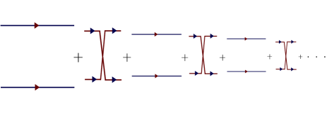
Figure 6: ”(Color online)” Diagrammatic scheme of the non-relativistic perturbative series. The even terms represented by two parallel lines correspond to the $\sigma_{z}$ coupling associated to a dynamical Stark shift term, whereas the odd terms depicted by crossing lines stand for the $\sigma_{y}$ interaction associated to a Ramsey interferometric effect. Note that the different scales stress the relevance of each term in the non-relativistic regime.

As we mentioned at the beginning of this appendix, the complete perturbative series can be interpreted in terms of the dynamical Stark shift term which accounts for the non-relativistic limit in section III, and the Ramsey interference term which accounts for the first order correction in section V. Therefore, the full phenomenology and the characterization of Zitterbewegung can be accomplished regarding these two regimes.

Finally, let us interpret the different terms of the so-called perturbative expansion with the language of Quantum Optics. The unitary operator in Eq. (53) describes the time evolution inside the invariant subspace $\mathcal{H}_{n_{l}}$ in Eq. (13). If we recover the full Hilbert space description, we obtain that the even terms of the perturbative expansion are

$$U^{2k}:=\lambda_{2k}\sin\phi_{n_{l}}(t)\left[\begin{array}[]{cc}(a_{l}^{\dagger}a_{l})^{k}&0\\ 0&-(a_{l}a_{l}^{\dagger})^{k}\\ \end{array}\right],$$ (54)

where $k=0,1...$ and we have introduced certain coupling constants $\lambda_{2k}(t):=c_{2k}\xi^{k}$ which involve increasing powers of the relativistic parameter, and $c_{2k}\in\mathbb{C}$ follow directly from Eqs.(51), (53). These terms represent a kind of dynamical Stark shift between the spinorial levels proportional to the $k-$th power of the orbital quanta number $n_{l}$. They might be considered as certain shifts produced by $2k$-virtual transitions between the spinorial levels.

In the same manner, we can rewrite the odd terms as

$$U^{2k+1}:=\lambda_{2k+1}\sin\phi_{n_{l}}(t)\left[\begin{array}[]{cc}0&(a_{l}^{\dagger}a_{l})^{k}a_{l}^{\dagger}\\ -a_{l}(a_{l}^{\dagger}a_{l})^{k}&0\\ \end{array}\right],$$ (55)

where the coupling parameter $\lambda_{2k+1}=c_{2k+1}\xi^{\frac{2k+1}{2}}$ becomes more important as the relarivistic parameter increases, and $c_{2k+1}\in\mathbb{C}$ also follow from Eqs. (51), (53). These perturbative terms (55) can be directly expresses as a generalized Anti-Jaynes-Cummings evolution

$$U^{2k+1}:=\lambda_{2k+1}\left(\sigma^{-}A_{k}-\sigma^{+}A_{k}^{\dagger}\right)\sin\phi_{n_{l}}(t),$$ (56)

where we have introduced the bosonic operator

$$A_{k}:=a_{l}(a_{l}^{\dagger}a_{l})^{k}.$$ (57)

This effective time evolution (56) can be interpreted as a generalized AJC-model where intensity of the couplings depends on the $k-$th power of the number of left-handed quanta $n_{l}$ knight ; vogel

References

- (1) M. Moshinsky and A. Szczepaniak, J. Phys. A 22, L817 (1989).
- (2) D. Ito, K. Mori, and E. Carrieri, Nuovo Cimento 51 A, 1119 (1967).
- (3) P. A. Cook, Lett. Nuovo Cimento 10, 419 (1971).
- (4) C. Quesne and M. Moshinsky, J. Phys. A 23, 2263 (1990).
- (5) M. Moreno and A. Zentella, J. Phys. A 22, L821 (1989).
- (6) J. Benitez, R. P. Martinez y Romero, H. N. Nuñez-Yepez and A. L. Salas-Brito, Phys. Rev. Lett. 64, 1643 (1990).
- (7) R. P. Martinez y Romero, M. Moreno, and A. Zentella, Phys. Rev. D 43, 2036 (1991).
- (8) E. T. Jaynes and F. W. Cummings, Proc. IEEE 51,89 (1963).
- (9) P. Rozmej, and R. Arvieu, J. Phys. A: Math. Gen. 32, 5367 (1999).
- (10) P. Rozmej, and R. Arvieu, Phys. Rev. A 50, 4376 (1994).
- (11) P. Rozmej, and R. Arvieu, Phys. Rev. A 51, 104 (1995).
- (12) P. Rozmej, and R. Arvieu, J. Phys. B: At. Mol. Opt. Phys. 29, 1339 (1996).
- (13) D. Leibfried, R. Blatt, C. Monroe, and D. Wineland, Rev. Mod. Phys. 75, 281 (2003).
- (14) A. Bermudez, M. A. Martin-Delgado, and E. Solano, Phys. Rev. A 76, 041801(R) (2007).
- (15) N. F. Ramsey, “Molecular beams”, (Oxford University Press, New York, 1985); Rev. Mod. Phys. 62, 541 (1990).
- (16) W. Greiner, “Relativistic Quantum Mechanics: Wave Equations”, (Springer, Berlin, 2000).
- (17) V. Villalba, Phys. Rev. A 49, 586 (1994).
- (18) There are two possible situations where the relativistic system is mapped onto the usual Jaynes-Cummings model jaynes_cummings . In an active procedure, the substitution in Eq. (3) leads to the chiral partner Hamiltonian of the Dirac oscillator which can be directly mapped onto a Jaynes-Cummings interaction bermudez_do_2D . Conversely, we may regard as the ground state and as the excited state, with a simultaneous change of sign in the detuning . This passive procedure is of no consequence since quantum optical detunings can experimentally attain both positive and negative values.
- (19) C. Cohen-Tannoudji, J. Dupont-Roc, and G. Grynberg, Atom-Photon Interactions. Basic Processes and Applications, (Wiley-VCH, Weinheim, 2004).
- (20) P. Meystre and M. Sargent III, “Elements of quantum optics”, (Springer-Verlag, Berlin, 1999).
- (21) A. E. Siegman, “Lasers”, (University Science Books, Sausalito, California, 1986).
- (22) M. Brune, S. Haroche, V. Lefevre, J. M. Raimond, and N. Zagury, Phys. Rev. Lett. 65, 976 (1990); M. Brune, E. Hagley, J. Dreyer, X. Maître, A. Maali, C. Wunderlich, J. M. Raimond, and S. Haroche, ibid. 77, 4887 (1996).
- (23) A. B. Klimov and L. L. Sánchez-Soto, Phys. Rev. A 61, 063802 (2000).
- (24) B. W. Shore and P. L. Knight, J. Mod. Opt. 40, 1195 (1993).
- (25) W. Vogel and R. L. de Matos Filho, Phys. Rev. A 52, 4214 (1995).